An Experimental Study of a Self-Supervised Classifier Ensemble

International Journal of Information Technology Volume 1 Number 1

An Experimental Study of a Self-Supervised Classifier Ensemble Neamat El Gayar

Using unlabeled data to enhance the performance of classifiers trained with few labeled data has been successfully applied in pattern recognition problems such as computer vision, human computer interaction, data mining, text recognition and classification. Using unlabeled examples for training has also been found useful in speech processing, object recognition, robotics and medical diagnostics. Other potential future applications include: content-based image retrieval, text understanding, classification in bio-informatics and more.

Abstract—Learning using labeled and unlabelled data has received considerable amount of attention in the machine learning community due its potential in reducing the need for expensive labeled data. In this work we present a new method for combining labeled and unlabeled data based on classifier ensembles. The model we propose assumes each classifier in the ensemble observes the input using different set of features. Classifiers are initially trained using some labeled samples. The trained classifiers learn further through labeling the unknown patterns using a teaching signals that is generated using the decision of the classifier ensemble, i.e. the classifiers self-supervise each other. Experiments on a set of object images are presented. Our experiments investigate different classifier models, different fusing techniques, different training sizes and different input features. Experimental results reveal that the proposed self-supervised ensemble learning approach reduces classification error over the single classifier and the traditional ensemble classifier approachs.

Unfortunately, several experiments have indicated that unlabeled data can cause a degradation in classifier performance [5], [6]. This has recently motivated further exploration of new more effective methods. The use of unlabeled data in classifier ensembles has gained little attention in the literature so far. Some of these attempts [7]-[9] have had preliminary success but report the need of further explorations of such methods.

Keywords— Multiple Classifier Systems, classifier ensembles, learning using labeled and unlabelled data, K-nearest neighbor classifier, Bayes classifier.

R

In this paper we introduce a new approach to learning using labeled and unlabeled data using a classifier ensemble.

I. INTRODUCTION

ESEARCHERS continue to focus on the design of pattern recognition systems to achieve the best classification rates.

The model proposed in this work integrates fusion techniques applied in classifier ensembles to generate teaching signals with which the different classifiers can learn, i.e can label their unknown patterns. We therefore refer to the proposed model as “self-supervised” learning model (SS).

Classifier ensembles –also often referred to as multiple classifiers- are often practical and effective solutions for difficult pattern recognition tasks and have gained momentum in the recent years [1]. Ensemble learning refers to a collection of methods that learn a target function by training a number of individual classifiers and then combining their decision. Classifier ensembles usually operate in parallel and learn only if labeled data is available.

Experimental results compare the proposed model to conventional classification techniques for an object recognition problem and investigate different classifier models, fusion techniques, training sizes and different input features. The paper is organized as follows: Section II, presents the architecture of the proposed self-supervised learning model using classifier ensemble. In section III, the data under investigation is presented and the feature extraction process is described. Section IV summarizes and discusses experimental results. Finally, the paper is concluded in section V.

Labeling training sets is a difficult and time-consuming task, which usually needs a skillful human expertise and can also be liable to errors. The problem of effectively combining unlabeled data with labeled data to enhance the performance of classifier is therefore of central importance in machine learning research. Among such efforts are found in [2]-[6]. Neamat El Gayar is with the Department of Information Technology, Faculty of Computers and Information, Cairo University, Giza, Egypt. (email:[email protected] or [email protected])

19

International Journal of Information Technology Volume 1 Number 1

Fuse Net Outputs + Generate Teaching Signal (o1, o op.., oP ) (t) t

o1

CL1

t

o2

CL2

CL2

feature vector x1

feature vector x2

t

oP

op

CLK

xp

xK

Object x

Figure 1 Self-supervised Classifier Ensemble

Figure 2 Columbia object Image DATA.

For the experiments using the classifier ensemble architecture, each image was divided into 2x2 segments and 3x3 segments resulting into 4 and 9 subimages, respectively. Each subimage was dealt with as a separate input image for a classifier in the ensemble architecture, as depicted in fig. 3. As follows we describe how features are obtained, and used as input to the classifiers from the raw images.

II. SELF-SUPERVISED LEARNING USING A CLASSIFIER ENSEMBLE The general architecture of the proposed self-supervised classifier ensemble (SS) paradigm is depicted in Fig.1 . It assumes an object is observed by different classifiers which process different features of the same object x. The classifiers ( CL1, CL2, ….. CLp, …… CLK) are trained using few labeled data samples for each feature stream.

A. Feature Extraction The image within the region of interest is divided into n x n non-overlapping sub-images and for each sub-image the orientation histogram of m directions(range: 0 - 2π, dark/light edges) is calculated from the gray valued image. The orientation histograms of all sub-images are concatenated into the characterizing feature vector.

Training proceeds as follows: After all K classifiers have been trained using the few available data samples, an unlabeled input vector x is observed. Each classifier, CLp processes its designated features of x, (xp) and produces an output op. The classifier outputs (o1, o2, ….. op, …… oK) are fused using known techniques to generate a teaching signal t. t can be viewed as a fuzzy label of the object x, i.e. each entry j of t would indicate to which degree pattern x belongs to class j (CLj). Learning using fuzzy labels can be found in [2] and will not be used in this work. From this fuzzy label, a hard label is generated, which corresponds to the class label with the highest value in t. This is the label assigned to the originally unlabeled pattern x. Repeating this procedure for all unlabeled data samples, a new labeled data set is generated. With this new labeled data set the single classifiers are trained further and their decision combined and the overall model tested.

2x2 input

Figure 3 Input images for the MCA

3x3 input

The gradient of an image f(x,y) at location (x,y) is the two

⎛ G x ⎞ ⎛ ∂f ∂x ⎞ ⎛ f * S x ⎞ ⎜ ⎟ ⎟ ⎜ G ⎟ = ⎜⎜ ∂f ∂y ⎟⎟ ≈ ⎜ f * S ⎟ y ⎠ ⎠ ⎝ ⎝ y⎠ ⎝

dimensional vector: ⎜

( * denotes the convolution operation). Gradient directions (Sx,Sy ) were calculated with 3 x 3 Sobel operators. The gradient directions are calculated with respect to the x-axis: α(x,y) = atan2 (f * Sy, f * Sy ) The atan2 function corresponds to the atan but additionally uses the sign of the arguments to determine the quadrant of the result. The m bins of the histogram all have equal size (2πm). The histogram values are calculated by counting the number of angles falling into the respective bin. Histograms are normalized to the size of their sub-images.

III. DATA AND EXPERIMENTS The data used for the experiments is a set of object images obtained from Columbia Object Image Library[10]. The dataset contains the images of 20 different objects, for each object 72 training samples are available. Fig. 2 illustrates examples of the 20 class image data used .

20

International Journal of Information Technology Volume 1 Number 1

IV.

Studying tables I and II, it is obvious that the SS approach outperforms both the single classifier approach and the MCS approach, with the SS(3x3) performing generally better than the SS(2x2). This is explainable by the fact that dividing the image into 3x3 regions, i.e 9 subimages leads to a bigger committee of classifiers which cause a better performance. Regarding the fusing rules, it can be seen that generally the median fusing rule perform best while the max fusing rule perform worse for the 3x3 data ( i.e for the MCS 3x3 and SS 3x3).

RESULTS

In this section, experimental results are presented. We mainly present the results of a K-nearest neighbor classifier (KNN) and a Quadratic Bayes Normal Classifier (QDC) [11]. KNN classifiers are popular for simplicity of use and implementation, robustness to noisy data and their wide applicability in a lot of appealing applications [12] On the other hand, Bayes classifiers are practical learning algorithms in which prior knowledge and observed data can be combined [13].

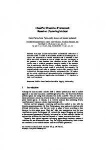
Fig. 4 and 5 illustrate previous results further by comparing the different approaches under varying the number of labeled patterns initially used for training for both Data 1 and Data 2, respectively, using the median fusing rule. It is obvious how the SS approach is superior, especially when few labeled samples are used for the initial training of the classifiers. Nevertheless, the performance of the models tends to become closer with the increase of number of labeled data samples used for training; which of course is an expected result.

Results compare following approaches using the KNN and the QDC classifiers: 1) The single classifier applied on the whole image data (referred to as “Normal” approach). The inputs to each classifier is the histograms obtained from processing the entire image of the object; as has been described in section III.A. 2) Two classifier ensembles (MCS); one that uses 4 classifiers (MCS 2x2) and another that uses 9 classifiers (MCS 3x3); each processing histograms of subimages of the object image (refer to sec. III.A). The decision of the classifiers are then combined using certain fusing rules.

Tables III and IV summarize the results obtained for the QDC classifier for Data 1 and Data 2, respectively. It is obvious that for the QDC the max fusing rule is not adequate. The performance of the QDC classifier has shown a big sensitivity to its regularization parameter to calculate the covariance matrix [11]. Here we used the regularization parameters [0.001,0.01], throughout the implementations to be uniform, which definitely did not guarantee the best performance for all classifiers. In spite of these difficulties results still indicate that the proposed SS approach improves the results.

3) Two self supervised classifier ensembles (SS); that learn using 4 and 9 classifiers and referred to as SS(2x2) and SS(3x3), respectively. Each single classifier is trained using the few labeled training samples and retrained using the newly labeled data set using the fused outputs of the classifiers as described in section II.

TABLE I K-NEAREST NEIGHBOR - ERROR % ON DATA 1 Data 1 Approach No of labeled patterns 20 30 40 Normal 23.24% 17.81% 14.32% MCS 2x2 Max 0.95% 0.06% 0.04% Mean 1.71% 0.44% 0.04% Median 1.10% 0.25% 0.04% Best_singl 9.96% 6.29% 3.81% MCS 3x3 Max 10.62% 9.24% 5.38% Mean 1.62% 0.29% 0.19% Median 1.04% 0.29% 0.06% Best sing 17.62% 11.19% 7.69%

For each implemented model the classifiers are trained using the same subset of the given training data and tested on the remaining data-points divided into two data sets ( Data 1 and Data 2). Results presented for each approach are the average over 5 different random choices of the training patterns and the test data sets. Tables I and II summarize the results obtained for the KNN classifier for Data 1 and Data 2, respectively. The tables compare the the classification error using different approaches: Normal, MCS(2x2), MCS(3x3), SS(2x2) and SS(3x3) when using 20, 30 and 40 training (i.e labeled ) data points out of the 72. For the MCS and the SS approaches the results of applying the max, mean and median fusing rules are also presented. The tables also list the classification error of the best single classifier (i.e the error of the best classifier before fusing the classifier outputs) for the MCS. This is always a good indication to check to which extent fusing the classifier decision improves results over each single classifier operating alone.

SS(2x2) Max Mean Median SS(3x3) Max Mean Median

21

0.27% 0.19% 0.15%

0.10% 0.05% 0.05%

0.00% 0.13% 0.06%

14.96% 0.23% 0.12%

11.43% 0.10% 0.00%

7.93% 0.00% 0.00%

International Journal of Information Technology Volume 1 Number 1

TABLE II K-NEAREST NEIGHBOR - ERROR % ON DATA 2 Data 2 Approach No of labeled patterns 20 30 40 Normal 21.55% 16.85% 13.29% MCS 2x2 Max 1.10% 0.27% 0.00% Mean 1.58% 0.35% 0.00% Median 1.23% 0.27% 0.00% Best_singl 10.12% 5.95% 4.19% MCS 3x3 Max 11.73% 9.00% 6.50% Mean 1.46% 0.43% 0.31% Median 0.65% 0.24% 0.06% Best sing 16.96% 10.91% 8.50% SS(2x2) Max Mean Median SS(3x3) Max Mean Median

0.65% 0.19% 0.08%

0.14% 0.05% 0.00%

0.06% 0.00% 0.00%

14.95% 0.23% 0.00%

11.16% 0.00% 0.00%

7.57% 0.00% 0.00%

TABLE III QUADRATIC CLASSIFIER - ERROR % ON DATA 1 Data 1 Approach No of labeled patterns 20 30 40 Normal 24.57% 22.94% 22.16% MCS 2x2 Max 7.38% 8.31% 9.33% Mean 2.33% 0.44% 0.08% Median 1.10% 0.13% 0.08% Best_singl 11.89% 9.86% 6.94% MCS 3x3 Max 34.32% 34.19% 34.50% Mean 2.46% 0.58% 0.05% Median 4.19% 3.94% 4.34% Best sing 18.46% 14.38% 14.75% SS(2x2) Max 12.27% 12.81% 12.50% Mean 0.46% 0.14% 0.00% Median 0.19% 0.29% 0.19% SS(3x3) Max 46.23% 43.48% 43.63% Mean 0.42% 0.14% 0.00% Median 5.31% 4.57% 5.44%

Knn, median fusing rule, Data 1 0.5

Normal

Error

0.4

MCS(2x2)

0.3

TABLE IV QUADRATIC CLASSIFIER - ERROR % Data 2 Approach No of labeled patterns 20 30 40 Normal 25.58% 23.65% 20.17% MCS 2x2 Max 7.81% 8.39% 9.67% Mean 1.87% 0.85% 0.00% Median 1.29% 0.65% 0.00% Best_singl 12.19% 9.19% 8.63% MCS 3x3 Max 35.20% 35.42% 35.29% Mean 2.67% 0.69% 0.00% Median 4.23% 4.19% 4.08% Best sing 19.39% 15.38% 13.25% SS(2x2) Max 11.73% 12.86% 11.81% Mean 0.23% 0.14% 0.00% Median 0.19% 0.14% 0.00% SS(3x3) Max 45.77% 43.76% 43.38% Mean 0.58% 0.14% 0.00% Median 6.12% 5.14% 4.94%

MCS(3x3)

0.2

SS(2x2)

0.1

SS(3x3)

0 5 10 15 20 25 30 35 40 45 50 no. of labeled patterns

Figure 4 Comparison of the different approaches using test data Data1

Knn, median fusing rule, Data 2

Error

0.5 0.4 0.3

Normal

0.2 0.1

MCS(3x3)

MCS(2x2) SS(2x2)

0 5 10 15 20 25 30 35 40 45 50

SS(3x3)

no. of labeled patterns Figure 5 Comparison of the different approaches using test data Data2

22

International Journal of Information Technology Volume 1 Number 1

V.

CONCLUSION AND FUTURE WORK

In this work, a classifier ensemble is proposed for learning using labeled and unlabeled patterns.. The model was tested on a set of objects images and compared to two approaches: the a single classifier applied to the whole image of the object and a multi- classifier approach applied to subimages. Experimental results using two different type of classifiers (KNN and QDC), two different division of the input features ( 2x2 and 3x3), different fusing rules and different number of initial labeled training patterns show that generally the selfsupervised classifier ensemble is able to enhance the classifier performance by effectively using the unlabeled data for training. Future work includes using adaptable classifier combination rules and applying the proposed model to real world application where labeled data is scare and unlabeled data is abundant and where it would be of crucial benefit to effectively use unlabeled data to enhance classifier performance. In our future work we also intend to integrate learning using fuzzy labels into the self-supervised learning model. REFERENCES [1]

J. Kittler, F. Roli and T. Windeatt (Eds.): Multiple Classifier Systems, Fifth International Workshop, MCS 2004 Cagliari, Italy, June 9--11, 2004, Proceedings. Lecture Notes in Computer Science, vol. 3077, Springer-Verlag Inc., NY, USA, 2004. [2] N. F. El Gayar. “Fuzzy Neural Network Models for Unsupervised and Confidence-Based Learning”, Ph.d. thesis, Dept. of Comp. Sc., University of Alexandria, 1999. [3] M. Seeger. “Learning with labeled and unlabeled data” (Technical Report). Institute for Adaptive and Neural Computation, University of Edinburgh, Edinburgh, United Kingdom,2001 [4] I. Muslea, S. Minton & C. Knoblock. “Active +semi-supervised learning = robust multi-view learning” Proc. of ICML-02, 19th Int. Conf. on Machine Learning (pp. 435–442) 2002. [5] X. Zhu, J. Lafferty & Z. Ghahramani “Combining active learning and semi-supervised learning using gaussian fields and harmonic functions”. Proc. of the ICML-2003 Workshop on The Continuum from Labeled to Unlabeled Data, Washington DC, 2003. [6] Ira Cohen, Nicu Sebe, Fabio G. Cozman,Thomas S. Huang, “Semisupervised learning for facial expression recognition” MIR’03, November 7, 2003, Berkeley, California, USA. [7] D. Miller and H.S. Uyar. "A mixture of experts classifier with learning based on both labeled and unlabeled data." NIPS 1997 [8] K.P. Bennett, A. Demiriz and R. Maclin. “Exploiting unlabeled data in ensemble methods” Proceedings of the eighth ACM SIGKDD international conference on Knowledge discovery and data mining, Edmonton, Alberta, Canada ., pp 289 – 296, 2002. [9] E. Dimitriadou, A. Weingessel and K. Hornik. “A mixed ensemble approach for the semi-supervised problem”, Proceedings of the International Conference on Artificial Neural Networks, pp 571 - 576 , 2002. [10] S. A. Nene, S. K. Nayar and H. Murase "Columbia Object Image Library (COIL-20)," Technical Report CUCS-005-96, February 1996. [11] R.P.W. Duin, P. Juszczak, P. Paclik, E. Pekalska, D. de Ridder and D.M.J. Tax, PRTools 4.0, A Matlab Toolbox for Pattern Recognition, Delft University of Technology, February 2004. http://prtools.org/ [12] R.O. Duda, P.E. Hart, D.G. Stork, Pattern Classification, 2nd ed., New York: John Wiley and Sons, 2001. [13] N. Friedman and R. Kohavi. “Data mining tasks and methods: Classification: Bayesian classification”, Handbook of data mining and knowledge discovery , pp. 282 – 288. Oxford University Press, 2002.

23