Root-MUSIC algorithm, designed for uniform linear arrays, has been extended to ... Index Termsâ DOA estimation, root-MUSIC, IDFT, manifold ..... 1939â1949,.
AN IDFT-BASED ROOT-MUSIC FOR ARBITRARY ARRAYS Jie Zhuang, Wei Li, and A. Manikas Department of Electrical and Electronic Engineering Imperial College London, SW7 2AZ, UK email: {jie.zhuang06, victor.li, a.manikas}@imperial.ac.uk ABSTRACT Root-MUSIC algorithm, designed for uniform linear arrays, has been extended to arrays of arbitrary geometry by means of manifold separation techniques but at the cost of increased computational complexity. In this paper, an inverse discrete Fourier transform (IDFT)-based method is proposed in which polynomial rooting is avoided. The proposed method asymptotically exhibits the same performance as the extended root-MUSIC, implying that it outperforms the conventional MUSIC in terms of resolution ability. A remarkable property of this algorithm is that it has a computationally efficient implementation because a finite number of IDFT operations can run in parallel. Index Terms— DOA estimation, root-MUSIC, IDFT, manifold separation techniques, arbitrary arrays 1. INTRODUCTION In array signal processing, the subspace-type techniques asymptotically exhibits infinite resolution capabilities and thus are classified as super-resolution techniques in estimating the direction-of-arrival (DOA). The MUSIC algorithm, the first subspace based approach, requires a search of the array manifold which may become computationally expensive. To alleviate this computational burden, the root-MUSIC algorithm, proposed in [1], reduces the DOA estimation to a problem of polynomial rooting by exploiting the specific geometry of uniform linear arrays (ULA). In [2], R¨ubsamen and Gershman have provided an excellent review and comparison of the existing techniques that can extend the root-MUSIC to arrays of arbitrary geometries. However, these extensions are achieved at the cost of increased computational complexity. This is because the degree of the polynomial is no longer defined by the number of array elements but it is a very large number that restricts the modeling errors to a wanted level. Thus in [2], an IDFT-based method, named line-search root-MUSIC, has been proposed. Nevertheless, the resolution ability of this method is inferior to the root-based methods [3]. In this paper, an improved IDFT-based algorithm is proposed, in which polynomial rooting is not required anymore and the computational complexity is reduced considerably due to the introduction of IDFT. Moreover, the resolution ability of the proposed method is asymptotically the same as the extended root-MUSIC. The following notation is used throughout this paper. Matrices are denoted by blackboard bold (e.g. A) or by boldface (e.g. r) symbols. Any column vector is represented by an underlined symbol (e.g. A, a). Italics denote scalars. The superscript (·)∗ , (·)T and (·)H denote complex conjugate, transpose, and conjugate transpose respectively. Furthermore, � · � denotes Euclidian norm of a vector, E{·} represents expectation operator, IN is a N × N identity ma-
978-1-4244-4296-6/10/$25.00 ©2010 IEEE
2614
trix, L[A] stands for the space spanned by the columns of A and the (m, n)th element of A is denoted by [A]m,n . 2. PROBLEM FORMULATION Consider an array of arbitrary geometry (planar or linear) operating in the presence of M uncorrelated narrowband signals. The N × 1 array received signal vector x(t) can be expressed as x(t) = Sm(t) + n(t)
(1)
where n(t) is the additive white Gaussian noise with covariance σn2 IN (σn2 is the noise power). The matrix S has columns the manifold vectors of the M signals, i.e., S = [S(r, θ1 ), S(r, θ2 ), ..., S(r, θM )]
(2)
where r is a matrix with columns the Cartesian coordinates of the sensors of the array and θ denotes the DOA. Note that only the azimuth angle θ ∈ [0◦ , 360◦ ), measured anticlockwise with respect to the positive x-axis, is considered in this paper. The vector m(t) has elements the M complex narrowband signal envelopes. Then performing eigenvalue decomposition on the second order statistics of x(t) yields � � H (3) Rxx = E x(t)x(t)H = Es Ds EH s + En Dn En where Es is the eigenvectors associated with the largest M eigenvalues and En represents the eigenvectors corresponding to the remaining small eigenvalues. The linear subspace L[Es ] and L[En ] are also known as signal subspace and noise subspace, which are mutually orthogonal. The diagonal matrices Ds and Dn have diagonal elements that are associated with the signal and noise eigenvalues respectively. Interestingly, by using the manifold separation technique [4, 5, 6], a N × 1 manifold vector can be expressed as S(r, θ) = G(r)d(θ) + ε
(4) N ×Q
where ε denotes the modeling error. The matrix G(r) ∈ C depends on array geometry only (For the details of G(r), see [4, 6]). The Vandermonde structured vector d(θ) ∈ C Q×1 is a function of the DOA only, defined as Q−1
d(θ) =
ej 2 θ √ [1, z, . . . , z Q−1 ]T 2π
(5)
with z = e−jθ . Theoretically, |ε| tends to zero as Q → ∞. In practical applications, Q can be safely replaced by a finite sufficiently large number (generally Q � N ) without generating significant modeling errors because �ε� decays superexponentially with
ICASSP 2010
where Bi (ρ) � bi ρ−i and k � i + Q. The number K, no less than (2Q − 1), takes the value of a power of 2. The coefficient B k (ρ) is defined as � Bk−Q (ρ), if 1 ≤ k ≤ (2Q − 1) B k (ρ) = (10) 0, if (2Q − 1) < k ≤ K
increasing Q. Then a polynomial is constructed as follows: p(z)
= =
� � S H (r, θ) En EH S(r, θ) n � � dH (θ) GH (r)En EH n G(r) d(θ) � �� �A
=
1 2π
Q−1
bi z
−i
(6)
i=−(Q−1)
where the coefficient bi is the sum of elements of A along the ith diagonal, i.e.,
bi = [A]m,n (7) ∀m−n=i
The polynomial p(z) has degree (2Q − 2), meaning that there are (2Q − 2) roots. The true DOAs correspond to the roots of (6) because theoretically S(r, θ) is orthogonal to the noise subspace L[En ]. Thus, for arbitrary arrays the DOA estimation is reduced to a root finding problem, in which DOAs can be obtained as the phase angles of the roots closest to the unit circle. This method is referred to as the extended root-MUSIC in this paper. Instead of spectral search, the extended root-MUSIC substantially reduces the computational complexity. However, the requirement of computing all the roots of (6), coupled with the fact Q � N , may render the extended root-MUSIC computationally expensive, particularly when the sensor number N is also very large. Next, an IDFT-based method will be proposed to reduce this computational burden. Note that in [2] an alternative technique, called Fourierdomain root-MUSIC, can also extend the root-MUSIC to arbitrary arrays, which yields a polynomial similar to (6). The proposed method, therefore, is applicable to both the manifold separation and Fourier-domain root-MUSIC techniques. 3. PROPOSED IDFT-BASED ROOT-MUSIC In practice, the roots of (6) are not exactly on the unit circle any more in the presence of perturbation, e.g, the effects of finite snapshots (finite observation interval). Even the slightest perturbation can result in the roots moving away from the unit circle (pp.209 of [7]). Therefore, it is reasonable to express the roots as z = ρe−jθ
(8)
where ρ denotes the radius. Following the work of [8], one can rewrite the polynomial in (6) explicitly dependent on θ and ρ by substituting (8) into (6) p(θ, ρ)
=
=
=
1 2π 1 2π
Q−1
bi ρ−i ejiθ
i=−(Q−1) Q−1
Bi (ρ)ejiθ
i=−(Q−1)
k=1
=
1 j(1−Q)θ e 2π
B k (ρ)ej(k−1)θ
(11)
k=1
and thus a 2-D spectrum is defined as PIDFT (n, ρ)
= =
1 2π(n−1) p( K , ρ) 2π/K K 1 j 2π (k−1)(n−1) K B k (ρ)e K
(12)
k=1
where n = 1, 2, . . . , K. Interestingly, the denominator of the above has the form of a typical K-point IDFT, meaning that the 2-D spectrum can be computed directly by using IDFT for a given ρ. Apparently the peaks of the 2-D spectrum correspond to the true DOAs because the roots of (9) are associated with the true DOAs. The DOAs can be estimated by the follows: θm =
2π(nm − 1) K
(13)
where nm is the index n of the mth peak. Please note that (12) can be rewritten in a compact form as PIDFT = F B ∈ C K×L
(14)
where L is the total number of circles required to scan. F ∈ C K×K is the inverse Fourier transform matrix and B ∈ C K×L denotes the coefficient matrix. That is, the elements of the three matrices in (14) are defined as follows: | [PIDFT ]n,� |
=
2π PIDFT (n, ρ� )
[F]n,k [B]k,�
= =
ej K (k−1)(n−1) B k (ρ� )
2π
(15a) (15b) (15c)
Thus, finding the peaks of (12) is equivalent to finding the minima of (14). Taking into account the Hermitian property of A (see (6)), one obtains that bi = b∗−i , which implies that p(z) is a Laurent polynomial [9]. According to Lemma 1 of [9], the roots of p(z) appear in conjugate reciprocal pairs, i.e., if z0 is a root of p(z), then (1/z0 )∗ is also a root of p(z). This implies that one only needs to find the roots inside the unit circle. In summary, the proposed IDFT-based root-MUSIC algorithm can be accomplished via the following steps. 1. Compute the matrix G(r). Note that this offline process requires to be done only once for a given array.
2Q−1 1 j(1−Q)θ
e Bk−Q (ρ)ej(k−1)θ 2π K
Then the magnitude of (9) is given by K 1
j(k−1)θ |p(θ, ρ)| = B k (ρ)e 2π
(9)
k=1
2615
2. Form the covariance matrix Rxx and perform eigenvalue decomposition to obtain the noise subspace En EH n and construct A in (6). Then the coefficient bi of the polynomial p(z) can be calculated from A using (7).
3. For ρ = 1, 1 − Δρ, 1 − 2Δρ, · · · until ρ = 1 − (L − 1)Δρ, do the following steps to scan the spectra along L circles. Δρ determines the grid of the circles. (a) Calculate the (2Q − 1) coefficients Bi (ρ) = bi ρ−i . Then the coefficients B k (ρ) can be obtained by padding Bi (ρ) with (K − 2Q + 1) zeros. (b) Perform K-point IDFT operation on B k (ρ) and invert the results to obtain the spectrum PIDFT (n, ρ) in (12) for the current radius ρ. 4. Identify the M peaks closest to the unit circle via 2-D search on the spectra.
Table 1. The roots of the extended root-MUSIC and (θ, ρ) pairs of the peaks of the proposed method, with both the root magnitudes and ρ within [0.5,1]. roots (θ, ρ) ◦ ◦ −0.0806 − 0.96j = 0.9634e−j94.8 π/180 (94.7◦ , 0.963) ◦ ◦ 0.0159 − 0.9596j = 0.9571e−j89.0 π/180 (88.9◦ , 0.957) ◦ −j282.1 π/180◦ 0.1467 + 0.6818j = 0.6974e (282.0◦ , 0.697) −j333.9◦ π/180◦ 0.5783 + 0.2839j = 0.6443e (333.7◦ , 0.644) −j12.1◦ π/180◦ 0.5997 − 0.1288j = 0.6134e (12.0◦ , 0.613) −j175.6◦ π/180◦ −0.5907 − 0.0452j = 0.5924e (175.5◦ , 0.592) −j222.2◦ π/180◦ −0.4344 + 0.3941j = 0.5866e (222.1◦ , 0.587) −j158.0◦ π/180◦ −0.5242 − 0.212j = 0.5655e (157.9◦ , 0.565)
5. Estimate DOAs by using (13). Remark A: If one scans the unit circle only, i.e., ρ is fixed at 1, then the proposed algorithm reduces to line-search root-MUSIC (LSroot-MUSIC) similar to that proposed in [2, 8]. LS-root-MUSIC is essentially identical to the conventional MUSIC, except that all spectral points of LS-root-MUSIC are calculated by a K-point IDFT operation while in MUSIC each point is obtained by a matrix multiplication. LS-root-MUSIC and MUSIC are under the assumption that, corresponding to each true DOA, there is a peak in the spectrum along the unit circle. This is a stronger assumption than distinct z-plane roots because the root-based methods are insensitive to the radial errors [3]. Hence, the proposed method is expected to have better resolution ability than LS-root-MUSIC and MUSIC. Remark B: The complexity order of the rooting in the extended root-MUSIC is O((2Q−1)3 ), assuming that eigenvalue-based methods are used for rooting. That is the roots are found by computing the eigenvalues of the corresponding companion matrix. The complexity order of LS-root-MUSIC is O(K log2 K). Each loop of Step 3 of the proposed method takes O(2Q) operations to compute the coefficient B k (ρ) and O(K log2 K) operations for K-point IDFT. Thus the overall complexity order of the proposed method is O(L(2Q + K log2 K)). It is important to point out that the spectra of the L circles can be computed simultaneously in parallel time O(2Q + K log2 K) using L processors, which is comparable to that of LS-root-MUSIC. For comparison, usual root-finding, e.g., eigenvalue-based method, is expected to be iterative which renders it difficult for parallel processing. In addition, despite the possible increase in computational complexity, the proposed algorithm generally offers greater estimation accuracy than LS-root-MUSIC. 4. NUMERICAL STUDIES Consider an arbitrary array of N = 5 sensors with x-y Cartesian coordinates (in units of half-wavelengths) given by the matrix � � 0, 1.0, 1.7, 1.5, 1.0 r= . 0, 0, 0.7, 1.5, 2.2 Let us assume that the array operates in the presence of M = 2 uncorrelated equally-powered signals with signal-to-noise ratio (SNR) 20dB. For the modeling error �ε� ≤ 10−15 , the length of d(θ) is Q = 99. The grid of the circles is Δρ = 0.001. The IDFT length K = 213 is chosen such that the quantization-error due to the limited angular grid step size is negligible. In the first example, 50 snapshots are obtained from one MonteCarlo realization with DOAs= [90◦ , 95◦ ], SNR=20dB. Then these
Fig. 1. For one realization, the spectra of MUSIC, LS-root-MUSIC and the proposed method (with ρ = 0.963 and ρ = 0.957) ,with the number of snapshots= 50, DOAs= [90◦ , 95◦ ], SNR=20dB.
data are processed by four methods: MUSIC, LS-root-MUSIC, the extended root-MUSIC and the proposed method. Figure 1 shows the spectra of MUSIC, LS-root-MUSIC and the proposed method (with ρ = 0.963 and ρ = 0.957). In Figure 2, the 2-D spectrum of the proposed method is demonstrated with ρ ∈ [0.5, 1] and Δρ = 0.001 (i.e., L=501). Note that in practice L is not required to be such a large number because empirically ρ ∈ [0.9, 1] is sufficient to locate the true DOAs. In Figure 1, one observes that MUSIC and LSroot-MUSIC fail as both provide only one peak at 93.9◦ , while the proposed method provides two peaks. The results of the proposed method are also shown in Figure 2 and Table 1, indicating that two DOAs are estimated (94.7◦ and 88.9◦ ). Note that the DOA estimations of the extended root-MUSIC are 94.8◦ and 89.0◦ . Therefore, the two root-based methods have better resolution ability than MUSIC-type methods in this example. Additionally, Table 1 indicates that the roots computed by the extended root-MUSIC, which no longer locate on the unit circle due to the perturbation, are in close proximity to the peaks of the proposed 2-D spectrum. Then two cases are considered, in which Monte-Carlo simulations of 1000 trials have been performed. Figure 3 indicates the DOA estimation root-mean-square-errors (RMSEs) of the four methods versus the number of snapshots, with DOAs = [90◦ , 95◦ ]. In Figure 4, the DOA estimation RMSEs versus the signal angular separation are presented, where the DOA of the second signal source varies from 91◦ to 100◦ while the DOA of the first signal is fixed at 90◦ . The two figures demonstrate that the proposed algorithm provides the asymptotically similar performance in DOA estimation to the extended root-MUSIC. Also, the proposed algorithm has superior capability to the two MUSIC-type approaches when two signal sources are closely spaced or the number of snapshots is quite small.
2616
Spectrum (dB)
Fig. 4. DOA estimation RMSEs versus (θ2 − θ1 ) with the snapshot number = 100, SNR=20dB, θ1 = 90◦ , ρ ∈ [0.9, 1] and Δρ = 0.001.
r
5. CONCLUSION
Azimuth (degree)
An IDFT-based root-MUSIC algorithm is proposed to estimate the DOAs by scanning a range of circles. This algorithm is computationally efficient as IDFT is adopted and it is possible to scan all circles in parallel processing. The analysis and simulation results verify that the proposed algorithm, with less computational burden, has asymptotically similar performance in DOA estimation to the extended root-MUSIC. Also, the proposed algorithm has superior resolution ability to LS-root-MUSIC and the conventional MUSIC, particularly when two signal sources are located close together in space or the number of snapshots is relatively small.
r
6. REFERENCES Azimuth (degree)
Fig. 2. The 2-D spectrum of the proposed IDFT-based method (and contour diagram), where the snapshots used is the same as that used in Figure 1. ρ ∈ [0.5, 1] and Δρ = 0.001 are used.
[1] A. Barabell, “Improving the resolution performance of eigenstructurebased direction-finding algorithms,” in Proc. Int. Conf. Acoustics, Speech, Signal Processing (ICASSP), Apr 1983, vol. 8, pp. 336–339. [2] M. Rubsamen and A.B. Gershman, “Direction-of-arrival estimation for nonuniform sensor arrays: From manifold separation to fourier domain music methods,” IEEE Trans. Signal Process.,, vol. 57, no. 2, pp. 588– 599, Feb. 2009. [3] B.D. Rao and K.V.S. Hari, “Performance analysis of root-music,” IEEE Trans. Acoust., Speech Signal Process., vol. 37, no. 12, pp. 1939–1949, Dec 1989. [4] M.A. Doron and E. Doron, “Wavefield modeling and array processing. i. spatial sampling,” IEEE Trans. Signal Process., vol. 42, no. 10, pp. 2549–2559, Oct 1994. [5] M.A. Doron and E. Doron, “Wavefield modeling and array processing .ii. algorithms,” IEEE Trans. Signal Process., vol. 42, no. 10, pp. 2560– 2570, Oct 1994. [6] F. Belloni, A. Richter, and V. Koivunen, “Doa estimation via manifold separation for arbitrary array structures,” IEEE Trans. Signal Process., vol. 55, no. 10, pp. 4800–4810, Oct. 2007. [7] T. Kailath, A. H. Sayed, and B. Hassibi, Linear Estimation, Prentice Hall, 1 edition, April 2000. [8] K.V.S. Babu, “A fast algorithm for adaptive estimation of root-music polynomial coefficients,” in in Proc. Int. Conf. Acoustics, Speech, Signal Processing (ICASSP), Apr 1991, pp. 2229–2232 vol.3.
Fig. 3. DOA estimation RMSEs versus the snapshot number with SNR=20dB, DOAs=[90◦ , 95◦ ], ρ ∈ [0.9, 1] and Δρ = 0.001.
2617
[9] A. H. Sayed and T. Kailath, “A survey of spectral factorization methods,” Numerical linear algebra with applications, vol. 8, no. 6-7, pp. 467–496, 2001.