pattern synthesis method using a steepest descent technique ..... From 1983 to 1986, she was a Research Engineer with the Georgia Tech. Research Institute ...
862
IEEE TRANSACTIONS ON ANTENNAS AND PROPAGATION, VOL. 47, NO. 5, MAY 1999
Pattern Synthesis for Arbitrary Arrays Using an Adaptive Array Method Philip Yuanping Zhou and Mary Ann Ingram
Abstract— This paper presents a new pattern synthesis algorithm for arbitrary arrays based on adaptive array theory. With this algorithm, the designer can efficiently control both mainlobe shaping and sidelobe levels. The element weights optimize a weighted L2 norm between desired and achieved patterns. The values of the weighting function in the L2 norm, interpreted as imaginary jammers as in Olen and Compton’s method, are iterated to minimize exceedance of the desired sidelobe levels and minimize the absolute difference between desired and achieved mainlobe patterns. The sidelobe control can be achieved by iteration only on sidelobe peaks. In comparison to Olen and Compton’s method, the new algorithm provides a great improvement in mainlobe shaping control. Example simulations, including both nonuniform linear and planar arrays, are shown to illustrate the effectiveness of this algorithm. Index Terms—Antenna array synthesis, array pattern synthesis, beamformer.
I. INTRODUCTION
O
VER the last several decades, there has been significant attention paid to the area of array pattern synthesis. A classic paper by Dolph [1] showed how to obtain the weights for an uniform linear array (ULA) to achieve a Chebyshev pattern, which is optimal in the sense that it yields a minimum uniform sidelobe level for a given mainlobe width. Other pattern synthesis approaches for ULA’s have been presented in literature [2]. A more challenging problem is to synthesize patterns for arrays with arbitrary element positions. Perini [6] proposed a pattern synthesis method using a steepest descent technique for nonuniform arrays. The algorithm iteratively updates the weights of array while searching for the point of minimum sum of squared errors between the synthesized pattern and the desired pattern. Ng et al. [5] developed a noniterative method norm using quadratic programming. Even to minimize the norms could be weighted as noted by Perini to though the emphasize certain portions of the pattern, there was no method given to adjust such weighting values in the iterative process. As a result, the abovementioned algorithms can guarantee neither a particular pattern shape in certain area nor a specific response level over a sidelobe region. Tseng and Griffiths [3] proposed an algorithm that iterates the constraints in the solution of a linearly constrained least square problem to control sidelobe peaks. Manuscript received April 12, 1998; revised December 10, 1998. The authors are with the School of Electrical and Computer Engineering, Georgia Institute of Technology, Atlanta, GA 30332 USA. Publisher Item Identifier S 0018-926X(99)04832-2.
A different approach to synthesis is to apply adaptive array theory. In an early paper, Sureau and Keeping [7] employed adaptive array techniques to synthesize the patterns for cylindrical arrays. The imaginary jammer powers were varied depending on desired sidelobe levels. Although they achieved reasonable sidelobe control, they did not provide a systematic approach to adjust jammer powers so that sidelobe levels could meet the desired specifications. Olen and Compton presented a systematic approach; a simple recursion is driven by the difference between the current synthesized pattern and the desired pattern over sidelobe regions [4]. The artificial interferers of various power levels are assigned in sidelobe regions to control sidelobe levels of the synthesized pattern. This algorithm is very effective and generally yields satisfactory array patterns. However, there is no pattern control mechanism in mainlobe region. In many applications, a mainlobe with a particular shape is desired, e.g., flat top. Without effective pattern control in the mainlobe region, specified pattern shaping can hardly be achieved. The mainlobe shaping problem might be fixed by applying constraints. However, when more constraints are used, the sidelobes become more difficult to control because the degrees of freedom are reduced due to the constraints. Furthermore, an additional matrix inverse is required when using constraints, which adds computational complexity and makes the algorithm slow if many patterns must be synthesized, for example, when pattern requirements change with look direction and multiple look directions are anticipated [12]. In this paper, we present a new pattern synthesis algorithm for arbitrary arrays based on adaptive array theory. The problems mentioned above can be eliminated completely with the new algorithm. The new algorithm shapes the mainlobe with an iterative procedure and employs an efficient sidelobe peak iteration technique to reduce computational complexity. We formulate the problem as finding the optimal array norm of the weight vector that minimizes the weighted difference between the synthesized pattern and the desired pattern. The difference between our algorithm and others that norm is that our algorithm iterates the values of use the the weighting function in order to minimize the exceedance the desired sidelobe levels and to minimize the absolute difference between desired and achieved patterns in the mainlobe region. This algorithm offers a high flexibility and can easily handle arbitrary arrays with nonisotropic elements. The new algorithm offers a significant improvement to Olen and Compton’s method [4] in regard to mainlobe shape control. Simulation results are presented to illustrate the effectiveness of this
0018–926X/99$10.00 1999 IEEE
ZHOU AND INGRAM: PATTERN SYNTHESIS FOR ARBITRARY ARRAYS USING AN ADAPTIVE ARRAY METHOD
863
Fig. 2. The reference pattern Pr (�).
where is the covariance matrix and correlation vector defined as
Fig. 1. An sidelobe canceler interpretation.
is the cross-
(5)
method. Following is the organization of this paper. Section II is the problem formulation, Section III describes the pattern synthesis algorithm, Section IV shows the simulation examples, and Section V is the conclusion.
(6) Furthermore, when constraints are needed, the pattern synthesis problem can be formulated as
II. THE PROBLEM FORMULATION The problem of array pattern synthesis can be stated as follows. Given the number of array elements and the element such positions, we want to find a set of complex weights has a maximum at the desired that the array pattern with a certain beamwidth and also the sidelobe direction levels meet the specified values. Let’s consider the sum of a weighted pattern errors over the set of angles
subject to where is the constraint matrix and is the constraint vector. The solution for optimal weight vector is (7)
(1)
The error
where
where
is found to be [10]
is the minimized error
(2) and is the steering vector of the array, is the conjugate is the th element pattern, transpose operation, is the reference pattern, is the weighting function, is the phase due to propagation where is is the th element position, and the wavenumber vector and is the weight vector. When the error is expressed as (3) may be interpreted as the average output we observe that power of a “sidelobe canceller” with main channel response to a collection of jammers (Fig. 1), where the th and the power . The key jammer has the location to this algorithm is that the jammer powers are adjusted to emphasize selected parts of the achieved pattern, particularly the mainlobe and sidelobe peaks. The weight vector that minimizes the error is the solution of a well-known least squares problem (4)
The array response at each angular location depends on . Different values of put the weighting function different emphasis on array responses at pertinent directions and, therefore, would result in a different array pattern. By large, our cost function makes it possible to making ensure sidelobe peaks are below a certain value. III. THE PATTERN-SYNTHESIS ALGORITHM A. Full Iteration The most common objective for pattern synthesis is to obtain a pattern with sidelobe level lower than a specified value over certain regions while maintaining a certain gain at , as look angle . Here, we select the reference pattern shown in Fig. 2, in which all the responses in sidelobe regions are zeros and the mainlobe peak response is a value A. The mainlobe shape is specified by the designer and could be, for example, a parabola. While it is impractical to have all zero sidelobe levels, we can induce lower and lower sidelobes by in selected areas. We increasing the weighting function to iteratively adjust use a realistic desired pattern until the sidelobe requirements in are met.
864
IEEE TRANSACTIONS ON ANTENNAS AND PROPAGATION, VOL. 47, NO. 5, MAY 1999
The weighting function is updated through an iteration procedure similar to that of Olen and Compton’s [4], which leads to a satisfactory array pattern. The iteration is as in (8) and (9), shown on the bottom of the page, where indexes the points in angle over which we are interested in and are the weighting controlling the pattern. function and the synthesized pattern, respectively, at the th is a small number for an error tolerance iteration and between the synthesized pattern and the desired pattern in is the desired pattern; and mainlobe region. are the iteration gains. Observe that for in the mainlobe is never decreased from its initial value. The region, is set up to facilitate the iteration process desired pattern is used to define the whereas the reference pattern pattern errors that are to be minimized. In general, and are the same in mainlobe regions but different in should be chosen sidelobe regions. The sidelobe part of according to a realistic specification or a reasonable estimation. to compute new weights. Let We next use and be the boundary points for mainlobe region, i.e. defines the mainlobe. Since the reference pattern is zero outside of this region, the cross-correlation vector and the covariance matrix become (10)
(11) is added to each diagonal element of where a small quantity the covariance matrix to prevent it from being ill conditioned [3]. Then the next weight vector is (12) and The iteration stops when the errors between are small enough in the mainlobe region and the sidelobe levels are equal to or lower than . of The procedure here is different from Olen and Compton’s method [4] in three respects: 1) the summation for here includes both mainlobe and sidelobe regions whereas only in [4]; 2) the crosssidelobe regions are included for here includes all or selected steering corelation vector vectors in the mainlobe region whereas only a single steering vector in the look direction is included in [4]; and 3) the iteration here occurs in both sidelobe and mainlobe regions whereas it only occurs in sidelobe regions in [4]. Mainlobe shaping is conveniently achieved by minimizing the output power (from the imaginary jammers) of the difference between two patterns (as in Fig. 1) rather than minimizing the output power of just the synthesized pattern.
Fig. 3. The initial pattern for the nonuniform linear array.
B. Peak-Only Iteration In this section, we consider an alternative form of the algorithm that iterates the weighting function values only in the mainlobe and on the peaks of the sidelobes. Originally, we thought that this version would be faster, and indeed the amount of computation per iteration is significantly reduced. However, the number of iterations increases, so this version takes about the same amount of time overall as the version discussed in the previous section. In spite of the lack of time savings, we include this form because it is easier to program than the original form and because it may inspire a future algorithm that has the sought-after time savings. We now motivate the alternative form. Suppose that the is some low but sidelobe part of the desired pattern admissible sidelobe level1. Then, if the original version of the algorithm is allowed to continue after the maximum sidelobe specification is met, we find that all weighting function values outside of the mainlobe go to zero except those on the peaks of the sidelobes. This happens because the polarity on the term in (8) becomes negative for all in the sidelobes that don’t correspond to peak locations. Eventually, the left argument of the max function becomes becomes zero. negative, and This phenomenon is illustrated for a 13-element nonuniform has a sidelobe linear array. The selected desired pattern level of 30 dB. Figs. 3–8 show the synthesized patterns along with the weighting functions at different iteration steps. The synthesis process starts with unity values of weighting function. It is clear that the values of weighting function will . This only exist on the peaks in sidelobe regions as suggests an alternative iteration scheme in which sidelobe 1 In
[13], we show how to identify the lowest admissible sidelobe level.
in mainlobe region in side lobe region if otherwise
(8) (9)
ZHOU AND INGRAM: PATTERN SYNTHESIS FOR ARBITRARY ARRAYS USING AN ADAPTIVE ARRAY METHOD
Fig. 4. The weighting function for the initial pattern.
Fig. 7. The synthesized pattern at the 16 336th iteration.
Fig. 5. The synthesized pattern at the 27th iteration.
Fig. 8. The weighting function at the 16 336th iteration
865
The peak sidelobe locations will generally change from iteration to iteration. Therefore, the updates in (10) and (11) in Section III are no longer appropriate because they keep the same set of angles throughout the synthesis procedure. We can rewrite (8)–(12) in a form that allows the update terms to involve only the angles of sidelobe peaks. The covariance matrix and cross-correlation vector can be expressed in terms and a residual crossof a residual covariance matrix , which are added to the current ones, correlation vector i.e., (13) (14) where Fig. 6. The weighting function at the 27th iteration.
levels can be sufficiently controlled by updating the weighting function only on peak sidelobe locations. To identify the locations of the sidelobe peaks, various peak-finding schemes are available. One of the easy ways to do it is to obtain peak locations by just comparing the neighboring response values.
(15) (16) is a residual weighting function that indicates how Here, much correction is needed for the mainlobe and the sidelobe
866
IEEE TRANSACTIONS ON ANTENNAS AND PROPAGATION, VOL. 47, NO. 5, MAY 1999
Fig. 9. An adaptive spatial filter model.
peaks at the current iteration.
is calculated as follows: in mainlobe in sidelobe peak (17)
2) Obtain an initial weight vector
, i.e.,
(20) in mainlobe (21)
where
(22) if otherwise. (18) The next weight vector is (19) With the exception of (17), the algorithm in (13)–(20) is equivalent to the previous one. The exception is that the update to the covariance matrix is done only for sidelobe peak locations. The pattern synthesis with this algorithm can be modeled as an adaptive spatial filter shown in Fig. 9. The inputs to this filter are the signals of unit amplitude with incident angle . The signal from each array element is weighted and then summed to give the array output, which is compared with desired array response over an angular range. The errors between the array outputs and the desired pattern are used to update the covariance matrix and the cross-correlation vector to obtain the next optimal weight vector. The adaptive algorithm minimizes the errors so that the synthesized array approaches the desired pattern . This pattern system is adaptive in the sense that the algorithm finds the next optimal weight vector depending on the new error environment. This adaptive filter model suggests the following step-bystep flow chart for programming implementation. signals of unit amplitude incident 1) Select inputs as from various angles; for example, from 90 to 90 with one-degree spacing.
is usually a small number; for example, 0.001. Here, from (2). Then obtain an initial array pattern 3) Find all peak sidelobe locations. Then obtain peak as well as some values of sidelobe values of in the mainlobe region at selected points of interest. 4) At selected points in mainlobe region and the points of sidelobe peaks, calculate the differences of . from the results of step (4) for pertinent 5) Calculate is specified to points using (17) and (18). Usually, , for example, and be much smaller than . Then, calculate and using (15) and (16). to the current covariance matrix , 6) Add to the current cross-correlation vector and also . Then obtain the next weight vector from (19). from (2). If it is satisfac7) Obtain the array pattern tory, stop; otherwise, go to step (3). The peak-only iteration scheme provides an alternative to the full iteration scheme. We found that peak-only iteration took less computational time for each iteration because the number of processing units involved in each iteration was greatly reduced. However, each iteration did not change the pattern as much compared to that of full iteration, therefore, more iterations were needed to obtain the same pattern. As a result, the overall computational times for both iteration schemes were about the same.
ZHOU AND INGRAM: PATTERN SYNTHESIS FOR ARBITRARY ARRAYS USING AN ADAPTIVE ARRAY METHOD
Fig. 10.
Initial pattern.
Fig. 12. Synthesized and Chebyshev patterns.
SYNTHESIZED PATTERN Element Nos. 1, 21 2, 20 3, 19 4, 18 5, 17 11
Fig. 11.
867
FOR A
TABLE I 21-ELEMENT NONUNIFORM LINEAR ARRAY
Position
65:0000� 64:6065� 63:8098� 63:2995� 62:8973� 0�
Element Nos. 6, 16 7, 15 8, 14 9, 13 10, 12
Position
62:3497� 61; 8494� 61:5302� 60:6299� 60:3749�
Intermediate pattern.
C. Two-Dimensional Pattern Synthesis This algorithm can be extended in a straightforward way to the synthesis of two-dimensional (2-D) array patterns. In the 2-D peak-only iteration scheme, the residual weighting funcbecomes tion at th iteration for the spatial location , where is an azimuth angle and is an elevation is replaced with in all previous expressions. angle. Fig. 13. The synthesized pattern.
IV. SIMULATION EXAMPLES In this section, we will show a few pattern synthesis examples using our algorithm. The array elements used in following examples are assumed to be isotropic although such an assumption is not necessary in our algorithm. No mutual coupling was assumed. Also, the peak-only iteration scheme is used in the examples. The first example is a Chebyshev pattern synthesis for a 15element uniform linear array with a half wavelength spacing. Fig. 10 shows the initial pattern, Fig. 11 shows an intermediate pattern and Fig. 12 is the final synthesized pattern along with the ideal Chebyshev pattern for the same array; the solid line is the synthesized pattern and the dashed line is the Chebyshev pattern. The patterns are almost identical. Here we selected
and . The reference pattern is chosen as the same as that in Fig. 2 except that there is only one specified value unity at the desired signal direction in the mainlobe region. The final synthesized pattern was realized in 23 iterations. The second example is to synthesize a pattern for a 21element nonuniform linear array with element positions shown in Table I. Fig. 13 shows the result using our method with in the mainlobe. In the third example, the synthesized pattern for a 41element nonuniform linear array has a flat top and a notch in the sidelobe region as shown in Fig. 14. Constraints can also be incorporated to place nulls in sidelobe regions by
868
IEEE TRANSACTIONS ON ANTENNAS AND PROPAGATION, VOL. 47, NO. 5, MAY 1999
Fig. 14.
Flat-top pattern with notch.
Fig. 15.
Multibeam pattern.
Fig. 16. Chebyshev/synthesized patterns.
Fig. 17. A nonuniform array.
using (7) instead of (4). The fourth example is a multibeam pattern synthesis for the same array as the third example. The synthesized pattern is shown in Fig. 15. In above two cases, Olen amd Compton’s method is not applicable because it does not provide any pattern control in the mainlobe region. The fifth example is to synthesize a 2-D Chebyshev pattern 5 rectangular uniform planar array of 25 elements for a 5 with half-wavelength spacing. The ideal Chebyshev pattern, shown as the solid line in Fig. 16 is used as both the reference pattern and the desired pattern. We used 1 spacing in azimuth from 0 to 180 and also 1 spacing in elevation from 90 to 90 for placing values of the weighting function. Fig. 16 also shows the lowest upper bound (dashed) and highest lower bound (dash) for all radial cuts of the synthesized pattern after 18 iterations. It is observed that the sidelobe peaks deviate from the ideal no more than 1.5 dB. The sixth example is to synthesize a 2-D pattern for a nonuniform planar array of 61 elements shown in Fig. 17. The reference pattern is a circularly rotated version of Fig. 2. The desired pattern is basically the same as the reference pattern except the sidelobe value is set to be a constant of and . 0.06 ( 24.437 dB). Also, we used
Fig. 18. Initial pattern.
The initial 2-D pattern is plotted in Fig. 18 as a function of and and a side view of the initial pattern is plotted in Fig. 19. The Figs. 20 and 21 show the two views of the final synthesized pattern.
ZHOU AND INGRAM: PATTERN SYNTHESIS FOR ARBITRARY ARRAYS USING AN ADAPTIVE ARRAY METHOD
869
function in both mainlobe and sidelobe regions insure a desired mainlobe shape as well as desired sidelobe levels. The weighting function iterations are driven by the difference between the synthesized pattern and desired pattern. In contrast to Olen and Compton’s method, the new method provides convenient mainlobe shape control. The algorithm has been demonstrated with simulations of nonuniform linear and planar arrays. REFERENCES
Fig. 19.
A side view.
Fig. 20.
Synthesized pattern.
[1] C. L. Dolph, “A current distribution for broadside arrays which optimizes the relationship between beam width and sidelobe level,” in Proc. IRE, vol. 34, pp. 335–348, June 1946. [2] R. J. Mailloux, Phased Array Antenna Handbook. Norwood, MA: Artech House, 1994 [3] C.-Y. Tseng and L. J. Griffiths, “A simple algorithm to achieve desired patterns for arbitrary arrays,” IEEE Trans. Signal Processing, vol. 40, pp. 2737–2746, Nov. 1992. [4] C. A. Olen and R. T. Compton Jr., “A numerical pattern synthesis algorithm for arrays,” IEEE Trans. Antennas Propagat., vol. 38, pp. 1666–1676, Oct. 1990. [5] B. P. Ng, M. H. Er, and C. Kot, “A flexible array synthesis method using quadratic programming,” IEEE Trans. Antennas Propagat., vol. 41, pp. 1541–1550, Nov. 1993. [6] J. Perini, “Note on antenna pattern synthesis using numerical iterative methods,” IEEE Trans. Antennas Propagat., vol. 19, pp. 284–286, Mar. 1971. [7] J. C. Sureau and K. J. Keeping, “Sidelobe control in cylindrical arrays,” IEEE Trans. Antennas Propagat., vol. AP-30, pp. 1027–1031, Sept. 1982. [8] L. Wu and A. Zielinski, “An iterative method for array pattern synthesis,” IEEE J. Ocean. Eng., vol. 18, pp. 280–286, July 1993. [9] D. H. Johnson and D. E. Dudgeon, Array Signal Processing: Concepts and Techniques. Englewood Cliffs, NJ: Prentice-Hall, 1993. [10] R. T. Compton Jr., Adaptive Antennas: Concepts and Performance. Englewood Cliffs, NJ: Prentice-Hall, 1988. [11] R. A. Monzingo and T. W. Miller, Introduction to Adaptive Arrays. New York: Wiley, 1980. [12] P. D. Anderson, M. A. Ingram, and P. Zhou, “Array pattern synthesis for satellite communications on-the-move,” in Proc. Asilomar Conf. Signals, Syst., Comput., Monterey, CA, Nov. 1996, pp. 50–54. [13] P. Y. Zhou, M. A. Ingram, and P. D. Anderson, “Synthesis of minimax sidelobes for arbitrary arrays,” IEEE Trans. Antennas Propagat., vol. 46, pp. 1759–1760, Nov. 1998.
Philip Yuanping Zhou received the B.S. degree in electrical engineering from Chongqing University, China, in 1982, and the M.S. degree in electrical engineering and computer science from the University of Illinois at Chicago in 1986. He is currently working toward the Ph.D. degree at the School of Electrical and Computer Engineering, Georgia Institute of Technology, Atlanta. From 1989 to 1994, he worked as an Engineer with MERET Optical Communications, Inc., Santa Monica, CA. His research interests include adaptive array processing, array pattern synthesis, and wireless communications.
Fig. 21.
A side view.
V. CONCLUSION We have presented two new pattern synthesis algorithms for arbitrary arrays, where iterations occur only in the mainlobe and on sidelobe peaks. The optimal weight vector is obtained by minimizing the sum of weighted squared errors between synthesized and desired patterns. Iterations on the weighting
Mary Ann Ingram received the B.E.E. and Ph.D. E.E. degrees from the Georgia Institute of Technology, Atlanta, in 1983 and 1989, respectively. From 1983 to 1986, she was a Research Engineer with the Georgia Tech Research Institute, doing signals and systems analyses of advanced radar systems and radar electronic countermeasure (ECM) systems. From 1986 to 1989 she was a Research Assistant with the School of Electrical Engineering, Georgia Institute of Technology, doing modeling and estimation of linear systems that are disturbed by random point processes. In 1989 she joined the faculty of the School of Electrical and Computer Engineering, Georgia Institute of Technology, where she is now an Associate Professor. Her research has included topics in wireless communications, array pattern synthesis, array signal processing, optical transmission systems, and radar systems.