paper presents a 0-1 integer linear programming (ILP) formulation for reliability-oriented high-level synthesis that addresses the soft error problem.
An ILP Formulation for Reliability-Oriented High-Level Synthesis S. Tosun*, O. Ozturk**, N. Mansouri*, E. Arvas*, M. Kandemir**, Y. Xie**, and W-L. Hung ** * Syracuse University **Pennsylvania State University * {stosun,namansou,earvas}@ecs.syr.edu **{kandemir,yuanxie,ozturk,whung}@cse.psu.edu Abstract Reliability decisions taken early in system design can bring significant benefits in terms of design quality. This paper presents a 0-1 integer linear programming (ILP) formulation for reliability-oriented high-level synthesis that addresses the soft error problem. The proposed approach tries to maximize reliability of the design while observing the bounds on area and performance, and makes use of our reliability characterization of hardware components such as adders and multipliers. We implemented the proposed approach, performed experiments with several example designs, and compared the results with those obtained by a prior proposal. Our results show that incorporating reliability as a first-class metric during high-level synthesis brings significant improvements on the overall design reliability.
1. Introduction One of the design challenges in nanometer VLSI era is the guarantees for reliability. With technology scaling, shrinking geometries, lower power voltage, higher frequencies and higher density circuits all have a negative impact on reliability: the number of occurrences of transient faults is increased due to those factors. A major source of the transient faults is soft errors, also called single event upset (SEU), which are induced through three different radiation sources: alpha particles from the naturally occurring radioactive impurities in device materials, high-energy cosmic ray induced neutrons, and neutron induced Boron10 fission [1]. Power-reducing techniques employed in many embedded systems make these systems more vulnerable to soft errors [2]. Therefore, there is a clear need for soft error-aware embedded system design. In order to have a robust design, the soft error problem must be addressed at different levels in a coordinated fashion, from high-level specification to low-level implementation. One of these levels that is particularly attractive and more beneficial is high-level synthesis (HLS), which is the process of determining the block-level (i.e., macroscopic) structure of the circuit. While the past work on HLS focused mainly on performance, area, and power constraints, reliability issues regarding soft errors have not received much attention. Consequently, there exist only a few prior HLS studies that targeted at detecting/correcting soft errors. A common characteristic of these techniques is that they employ duplication (under performance/area bounds) during HLS to increase resilience to soft errors. Prior work has investigated soft error susceptibility of memory elements and combinational circuits [3]. They showed that combinational circuits are less susceptible to soft errors than memory elements. This is because of three major error masking effects on combinational circuits; namely logical, electrical, and latching-window masking. On the other hand, Sivakumar et al [4] demonstrate that the soft error susceptibility of combinational circuits will be comparable to that of memory circuits by the year of 2011
with the current technology trends. This significant prediction urges the computer designers for further research to reduce the soft error effects on data-path part of the designs since the current protection techniques for combinational circuits introduce more area, power consumption, and/or performance penalty than those designed for memory elements. These observations motivate us to consider the effects of soft errors on the problem of high-level data-path synthesis and the overall reliability for the combinational part of the resulting designs. Therefore, the work proposed in this paper is orthogonal and complementary to techniques for improving reliability of memory components. In this paper, we take a fresh look at the soft error-aware HLS problem, and present an approach based on integer linear programming (ILP). As against the duplication-based prior work in this area, we assume the existence of multiple versions of a given operator (a node in the data-flow graph), each varying in terms of performance, area, and reliability metrics. Our approach, using ILP, determines the most suitable (i.e., most reliable) version for each data-flow graph node under the given area and performance bounds. We also evaluate the overall reliability of the resulting high-level design. To test the effectiveness of our approach, we automated it within a custom HLS tool that performs scheduling, resource sharing, and binding. Our experimental evaluation using a set of sample designs demonstrate that the proposed approach improves the overall design reliability significantly, over a soft error-oblivious alternative. We also compare the resulting designs from our implementation with those obtained through a prior work that considers only node duplication, and discuss why a unified approach that integrates both of these techniques can generate better results than each individual scheme. The rest of this paper is structured as follows. The next section discusses the related work on ILP-based HLS and reliability-aware HLS. Section 3 presents background on soft errors, discusses our library characterization, and explains the reliability mechanism employed to evaluate the overall design reliability. Section 4 gives the problem definition for reliability-oriented HLS, and presents our ILP formulation. Section 5 gives our experimental evaluation, and finally Section 6 concludes the paper.
2. Related work Most of the prior work on formulating the HLS problem using ILP mainly focused on area-performance or area-performance-power tradeoffs. Achatz modeled the high-level synthesis problem using extended 0-1 linear programming [5]. His model handles the multifunctional units as well as units with different execution times under time-constraint or resource-constraint. OSCAR system [6] also makes use of 0-1 integer programming for solving scheduling, binding, and allocation. Since the number of variables and inequalities in the ILP formulation can grow exponentially, applying ILP to large problems may be problematic. To reduce the computation time of the
1
algorithm, [7] presented an in-depth analysis, and proposed a well-structured ILP formulation for the HLS problem. Several studies also investigated the module selection problem using ILP such as [5]. All of the studies mentioned above consider only area and performance optimizations. There has not been any prior ILP based formulation, to the best of our knowledge, considering reliability as a first class citizen in HLS framework along with area and performance constraints. However, there exist some publications in this context that use heuristic methods [8] [9]. These studies on reliable circuit design make use of component redundancy. They typically use one resource (version) for each type of operation with a fixed reliability, and the overall design reliability is increased by adopting N Modular Redundancy (NMR). In [8], Orailoglu and Karri introduced a design methodology for fault-tolerant ASICs. They presented two strategies that are based on NMR. The first strategy targets at minimizing the overall cost of the design under performance and reliability constraints, while the second one tries to maximize the reliability given the cost and performance constraints. Another method used to improve the reliability of the high-level system is to duplicate the entire structure for the fault-detecting circuits [10]. Studies using this method copied the entire flow graph, and subsequently used various strategies to minimize the overall area requirements of the final design. For example, [10] exploited the freedom of operations in data-flow graph, and scheduled both the copies to reduce the area overhead. Our approach differs from these previous studies since it makes use of a reliability-characterized library that has different versions of resources with different area, performance, and reliability metrics. The library we use permits us choose the most reliable resources for a specific task. In other words, instead of increasing reliability through redundancy, we achieve reliable design by using different versions of the components (to the extent allowed by area and performance bounds). In addition, our approach is based on ILP, rather than heuristic techniques.
3. Soft errors and reliability In this section, we briefly discuss soft errors and explain our library characterization method based on soft error rate in a component. We also present the mechanism used to calculate the reliability of a design.
3.1. Background on soft errors A soft error, also called Single Event Upset (SEU), is an error that is induced through different radiation sources. It causes to have a glitch on the circuit, usually resulting in a transient fault in the device. Soft errors occur when the collected energy Q at a particular node is greater than a critical charge Qcritical. Soft Error Rate (SER) can be estimated using the concept of critical charge. Hazucha and Svensson [11] proposed the following model to estimate the SER:
SER ∝ N flux × CS × exp
− Qcritical , Qs
(1)
where Nflux is the intensity of the neutron flux, CS is the area of cross section of the node, and Qs is the charge collection efficiency that depends on doping. The SER of a component can be reduced by improving a parameter in Expression (1). For example, there have been studies [2][12] demonstrating how supply voltage (threshold voltage) can affect the SER of a component. Experiments in these studies show that increasing the
supply voltage may improve SER. However, it also adversely affects the robustness of combinational logic. Therefore, one may need to approach to the design process from a different angle to improve the reliability of the final Soft error susceptibility of different product. implementations of a component may vary for each version. Consequently, these components may have different reliability characteristic, which will be detailed in the following subsection. Based on this, we direct ourselves to find more reliable designs by using available components instead of changing any parameters in Expression (1) and not affecting the hardware quality of the components. By doing so, our approach brings better reliability to the final design while not reducing its quality.
3.2. Reliability characterization based on soft errors Current library characterization efforts [13] focus mainly on latency, area, and power. However, it is equally important to study the soft error susceptibility of library components so that one can conduct a tradeoff analysis between reliability and other metrics, which is critical for our purposes. Efficient soft error fault injection and simulation techniques [14] can be used to evaluate the soft error susceptibility of a library component. Specifically, for each component, each of the nodes (gates) in the netlist can be characterized individually to determine their soft error susceptibility by fault injection and simulation. After this step, by analyzing the interconnection of gates in the netlist, the overall soft error susceptibility of the design can be determined. For our resource library, we implemented three different adders (ripple-carry adder, Brent-Kung adder, and Kogge-Stone adder) and two multipliers (carry-save multiplier and Leap frog multiplier), each having different area, performance, and reliability characteristics. We use a three-step approach illustrated in Figure 1 to estimate the reliabilities of these components and their different implementations. In the first step, we derive the Qcritical values from circuit simulation. For example, we determined the Qcritical values for ripple-carry, Brent-Kung, and Kogge-Stone adders as 59.460e-21 C, 29.701e-21 C, and 37.291e-21 C, respectively. Then, using these Qcritical values for each implementation, we estimate the SER values for the corresponding implementations using Expression (1). With the same technology generation, Nflux and CS can be chosen to be the same for different circuit implementations. With the assumption of uniform neutron flux [2], Qs can also be chosen to be same for two circuits. Thus, the SERs for two circuits that perform the same functionality can be related to each other as follows: Q − Qcritical 2 SER1 = SER2 * exp{ critical1 }. (2) Qs SER ∝ Nflux ×CS × exp −Qcritical Qs Qcritical
SER
1 2
Reliability
3
λ = SER
Failure rate
R(t) = exp{−λ t}
Figure 1. Qcritical, SER, failure rate, and reliability relationship.
2
The next step is to relate the SER of each component to its reliability. Reliability is defined as the probability with which a component will perform its intended function satisfactorily for a period of time [t0,t], given that the component was working properly at time t0. To calculate the reliability of a design, we should determine its failure rate , which is the probability with which the design will fail in the next time unit, given that it has been working properly in the current one. We can relate the reliability of a component to its failure rate by the following distribution function: R(t ) = exp{−λt} . (3) We use the SER of a component as its failure rate, assuming that every soft error will result in a failure. This is shown as the second step in Figure 1. Then, we determine the reliability of a component, which is the third step in the same figure. Note that the reliability of the ripple-carry adder is set to 0.999; and the reliabilities of other components are determined based on this value, using three steps depicted in Figure 1. We used the MAX layout editor tool and the HSPICE simulator to implement and simulate the different versions of components. Table 1 shows the normalized delay and area values under columns two and three, respectively. The column four gives the reliability values for each resource; estimated using the steps explained above. Since we want to compare our approach with a redundancy-based solution, we performed experiments with duplicated resources as well. The area of a duplicated resource is assumed to be twice the size of its original (non-duplicated) version, ignoring the area of interconnection and the checker circuitry. The reliability of a duplicated resource can be calculated using the following equation: Rd = R1 + R2 − R1 R2 (4) For example, while the reliability of adder 1 is 0.999 without any redundancy, its duplicated version has a reliability of 0.999999. The area and reliability values of the duplicated resources are shown under the columns five and six of Table 1. In all of our experiments, we use the values given in this table.
Inputs to our high-level synthesis framework are a data-flow graph and a resource library. The data-flow graph is a polar directed acyclic graph G(V,E), where the sets V={vi; i=0,1,…,n} and E={(vi,vj); i,j=0,1,…,n} are the vertex (node) set and edge set, respectively. While the vertex set represents the one-to-one correspondence between the operations and nodes, the edge set represents the data dependencies among nodes. The second input to the framework is the resource library, given in Table 1. Each resource in this table differs from other resources by having different area, delay, and/or reliability values. Note that we also have multiple implementations of a resource with different area, delay, and reliability values in this resource library. There are also area and performance constraints (represented by A and L, respectively) that are specified by the designer. The resulting design must satisfy both the area and performance constraints. The problem addressed by the reliability-oriented HLS is to schedule the data-flow graph with available resources such that the area and performance constraints are met and the reliability of the overall design is maximized. To achieve this, our HLS framework selects the most reliable resources from the resource library, observing the bounds.
3.3. Design Reliability
4.2.
In order to compare the reliability of two alternate designs with potentially different versions of resources, we need a mechanism to evaluate the overall reliability of a design. In high-level synthesis, to have a successful execution of an entire design, all the components of the design must succeed (i.e., operate without failure). Therefore, to express the reliability of the design, we adopt the following formula:
To make our ILP formulations easy to follow, we start by presenting the notation used in our formulations. Table 2 lists the constants and variables used, and their definitions. For the unified scheduling and binding problem, we define two binary decision variables subscripted using two indices X = {xis; i=0,1,…,n; s=1,2,..,L+1} and B = {bir; i=0,1,…,n; r=1,2,…,m}, where the first index for both the variables represents the name of the node (vertex), including source (v0) and sink (vn) vertices. The second index in variable x represents the start time of the operation. We start by scheduling the source node at cycle 1, and schedule the sink node at a given latency L plus one (L+1). The indices in variable x indicate which operation will start at which cycle; i.e., xis is one if and only if node i starts at step s. In variable b, r indicates the resource that can be mapped to node i. Note that the resource library can provide a very large number of resources for an operation, which can be used by our approach as long as the resulting design is within the bounds as indicated by the total area constraint. The indices in variable b indicate which node is bound to which resource type; i.e., bir is one if and only if node i is bound to resource r. After having defined the variables and constants used in
n
Rs = ∏ Ri
(5)
i =1
Table 1. Area, delay, and reliability values for different adder and multiplier versions. Resource type Adder 1 Adder 2 Adder 3 Multiplier 1 Multiplier 2
Delay (cc) 2 1 1 2 1
Without duplication Area (Unit) 1 2 4 2 4
Reliability 0.999000 0.969000 0.987000 0.999000 0.969000
With duplication Area (Unit) 2 4 8 4 8
Reliability 0.999999 0.999039 0.999831 0.999999 0.999039
It should be emphasized that we only consider non-hierarchical data-flow graphs in our experiments, i.e., we use data-flow graphs that do not contain any branching or iteration constructs.
4. Problem definition and ILP formulation In this section, we define the problem of reliability-oriented high-level synthesis, and explain our 0-1 ILP formulation for the stated problem. ILP is usually used in the optimization problems, in which every function must be linear, and solutions to each variable must be integers. If each variable is restricted to be either 0 or 1 in the ILP, it is called 0-1 ILP, which also known as ZILP.
4.1.
Problem definition
ILP formulation
3
TABLE 2. The constants and variables used in our ILP formulation. Notation L A n m ar Rr Ni tr dj T yr xis bir
kisr
Definition Maximum allowable latency Maximum allowable area Number of nodes in the data-flow graph Number of resources in the resource library for each type Area of resource r Reliability of resource r Reliability of node i Delay of resource r Delay of node j Overall reliability of the design Number of type r resources used in the design Variable associated with scheduling information of node i xis is 1 if and only if node j is scheduled to step s; 0 otherwise. Variable associated with binding information of node i bir is 1 if and only if node i is bound to resource r; 0 otherwise. Variable associated with scheduling and binding information of node i kisr is 1 if and only if node i is scheduled in step s and bound to resource r; 0 otherwise.
∀r :
∀i :
s =1
0≤i≤n
xis = 1;
m r =1
0≤i≤n
bir = 1;
m r =1
0≤ j≤n
t r b jr ;
L +1 s =1
s ⋅ xis −
L +1 s =1
s ⋅ x js − d j ≥ 0;
(12)
0 ≤ i ≤ n; 1 ≤ s ≤ L + 1; 1 ≤ r
m r =1
(6)
(8)
(10)
In order to ensure correct scheduling, the sequencing constraints must also be satisfied. A sequencing constraint states that the start time of operation i must be larger than or equal to the start time of any of its immediate predecessor j plus dj.
∀i, j :
0≤i≤n
After this, the kisr values are plugged into the left hand side of Expression (12) so that the formulation becomes linear. After finding the instances of each resource, the total area of the design is found by adding the product of the areas of resources and their instances used in the design by Expression (14). Obviously, the total area consumption must be bound by A.
Note that in this formulation, we only bind the nodes to the resources with corresponding type. We also require each variable b to be a non-negative integer: bir ∈ {0,1}; 0 ≤ i ≤ n; 1 ≤ r (9) Since our resource library has multiple implementations of a given operation type, there are multiple possibilities for a node’s execution delay. Thus, we use the following expression for expressing the delay of each node:
dj =
xis bir ≤ y r ;
Since a linear solver cannot solve the non-linear inequality given in Expression (12), we define a variable with three indices, kisr such that kisr is 1 if node i is scheduled at step s, and is bound to resource r. This variable can be expressed as follows: ∀i, s, j : xis + bir − 1 ≥ k isr ; (13)
We also require each x variable to be a non-negative integer: xis ∈ {0,1}; 0 ≤ i ≤ n; 1 ≤ s ≤ L + 1 (7) We then need to formulate the binding information. Each operation in the final design should be bound to one and only one resource, which can be expressed as follows [15]:
∀i :
L s =1
the formulation, we can now present the constraints and objective functions. First, we formulate the start time of each node. In the schedule, each operation has to be started once. Consequently, the following standard expression states this constraint [15]: L +1
resource used in the schedule to determine the total area of the design. The following expression is used for this purpose:
(11)
0 ≤ i , j ≤ n : ( vi , v j ) ∈ E Finally, we have to express the area constraint. To do this, we have to find the maximum number of instances for each
ar yr ≤ A
(14)
Having specified the necessary constraints, we next give our objective function, which aims to maximize the overall reliability of the design. To do this, we should assign the reliabilities of corresponding resources to each node:
Ni =
m r =1
0≤i≤n
Rr bir ;
(15)
Then, we need to determine the reliability of the overall design by multiplying the reliabilities of each node, as shown in Expression (16). However, this equation cannot be solved by any ILP solver since it is a non-linear function. n
MAX:
T = ∏ Ni
(16)
i =0
Alternatively, we may have used a logarithmic equation, given in the following expression: n
n
i =0
i =0
log T = log(∏ N i ) =
log N i
(17)
This equation may serve for the same purpose as Expression (16). However, we also need to re-write Expression (15) in a logarithmic fashion to be consistent with Expression (17). Since the logarithmic terms could not be used in Expression (15), we use the summation of the reliabilities of each node, instead of taking their product as our objective function. This can be expressed as follows: MAX:
T=
n i =0
Ni
(18)
We calculate the total reliability of the design after our ILP solver gives a solution. For the example designs we tested, we verified by hand that Expressions (16) and (18) result in the same final design. In fact, since the reliability values of the components are very close to 1 (one), Expression (18) can be employed safely to find the optimal designs. We implemented the ILP formulations using a publicly available Mixed Integer Programming (MIP) solver [1].
5. Experimental results In this section, we present experimental results
4
illustrating the impact of the proposed approach by comparing it with an alternate scheduling scheme. We also compare our resulting designs with those obtained from the prior work that employs redundancy-based reliability enhancement. In our experiments, we used two high-level synthesis benchmarks: an autoregressive lattice filter (AR) and a 16 point elliptic wave filter (EW). For the resource library, we use the resources listed in Table 1. We first illustrate the impact of our approach on two different designs, i.e., the AR, and EW filters. Then, we present a comparison of our approach with the solution presented in [8]. We also show the results when our approach is combined with the method presented in [8]. Note that, we employ duplicated resources only in the last experiment. In the first experiment, we schedule the AR filter with two different approaches. Figure 2(a) shows the first approach that uses only one implementation (version) for each type of operator (node). We choose this scheduling scheme to show how our approach benefits from employing multiple implementations of components. In Figure 2(a), specifically, we restrict ourselves to type 3 adders and type 2 multipliers, and perform scheduling and binding without considering reliability. Note that, if we have used other adder or multiplier versions, we would not be able to meet the area or performance constraint. In comparison, the scheduling resulted from our reliability-oriented approach is shown in Figure 2(b). The latency and area bounds for these two designs are 8 clock cycles and 24 units, respectively. The resulting area for the first design is 24 units (two adders of type 3 and four multipliers of type 2), while its reliability is 0.5164. On the other hand, our design has a reliability of 0.5834, representing a 13% improvement over the first design; and its area is the same as the first schedule. To achieve higher reliability, our solution uses one adder of type 1, one adder of type 3, four multipliers of type 1, and one multiplier of 2. The adders of type 3 in Figure 2 and Figure 3 are filled with darker color to distinguish them from the adders of type 1. In our next experiment, we evaluate two possible schedules for the EW filter with a 14 clock cycles of latency and 8 units of area bounds. The two schedules are illustrated in Figure 3. The schedule in Figure 3(a) results in a reliability of 0.455087, requiring an area of 6 units (three adders of type 2). Note that, we cannot employ other versions of adders for this experiment if we are to meet the specified area and performance constraints. Our approach (shown in Figure 3(b)) leads to a total area of 8 units (two adders of type 1, one adder of type 2, and one adder of type1), and achieves an overall reliability of 0.80767, a 77% improvement over the first schedule.
Step 1
x1
x2
x3
x4
Step 2
+5
+6
Step 3
+7
+8
Step 4
Step 7 Step 8
x17 x18
x2
x3
x4
+5
+6
+7
+8
x17 x18 x16
x10
x11
x9
x12
+24
x10
x11
x9
x12
+24 x15
+14
+13
Step 5 Step 6
x1 x15
x20
x21
x22
x19
+25
x16 +23
+28
(a)
x20
+14 x21
x19
+25
+26 +27
+13
x22
+23
+26 +27
+28
(b)
Figure 2. Two possible schedules for AR filter with L=8 and A=24.
Step 1
+1
Step 2
+3
+3
Step 3
+4
+4
+2
+1
+2
+5
Step 4 +6
Step 5
+6 +8
Step 6
+13
Step 11
+15
+18
+19
+17 +16
+11 +13
+21 +15
+14
+16 +22
+18 +23
Step 13
+25
+9
+24 +9 +26 +12
(a)
+17
+19
+20
Step 12
Step 14
+8 +10
+14
Step 9 Step 10
+7
+10
+11
Step 7 Step 8
+5 +7
+20 +21
+23 +24
+22
+12 +25
+26
(b)
Figure 3. Two possible schedules for EW filter with L=14 and A=8.
These two examples show two important contributions: Incorporating reliability as a first-class parameter into the HLS brings significant improvements on the overall design reliability, and By employing multiple implementations of resources, each having different reliability characteristic, one can improve the reliability of final design. In our last experiment, we make two comparisons. First, we compare our method with the one proposed in [8] by scheduling the AR filter with various area and performance bounds. The reason we compare our approach with [8] is that it uses reliability as a numerical metric as our approach does, and to the best of our knowledge, it is the only study in this context prior to our research. While the method presented in [8] uses redundancy to improve overall design reliability, we do not employ any redundancy in our designs. Our second comparison is designed to show the impact of a unified scheme (i.e., we combined the method proposed in [8] and ours). Specifically, we use redundancy (based on [8]) following our solution explained in this paper as far as the area constraint permits. That is, first, our approach finds a solution without duplication, and then we add redundant resources as long as we meet area bound. Then, we compare the results of this unified scheme with those obtained through [8]. The results from this experiment are shown in Table 3. The columns one and two in this table list the specified latency and area constraints, respectively. The column three shows the reliability values obtained by [8], and the column four gives our overall design reliabilities. The column five gives the percentage reliability improvement provided by our method over [8]. As can be observed from this column, our method obtains more reliable designs most of the time, even though we do not exploit any redundancy. However, as we start increasing the area bound, the reliability values found by [8] also increase and start to outperform our method. Note that, a negative value in this column means that the reliability value obtained by [8] is better than ours. The reason for negative values is that when we have tight performance and area bounds and we have to choose the most reliable resource for an operation, [8] selects a
5
TABLE 3. Reliability values and improvements under different latency and area bounds. L
Bounds A
Ref [8]
Our method
Imprv (%)
Our method + [8]
Imprv (%)
Solution time(s)
9 9 9 9 9 9 9 10 10 10 10 10 10 11 11 11 11 11 11 12 12 12 12 12 12
20 21 22 23 24 25 26 12 13 14 15 16 18 12 14 16 18 20 22 12 14 16 18 20 22
0.4140 0.4140 0.5127 0.5127 0.5972 0.5972 0.6013 0.4140 0.4140 0.5127 0.5127 0.5972 0.6545 0.4140 0.5127 0.5972 0.6545 0.7624 0.8356 0.4140 0.5127 0.5972 0.6545 0.7624 0.8356
0.4140 0.4400 0.4971 0.5284 0.5655 0.6011 0.6392 0.4140 0.4537 0.4822 0.5284 0.5969 0.6666 0.6744 0.7168 0.7715 0.8616 0.8616 0.8616 0.6744 0.7619 0.8201 0.8827 0.8827 0.8827
0 6.29 -3.02 3.07 -5.31 0.64 6.30 0 9.58 -5.94 3.07 -0.05 1.86 62.88 39.81 29.19 31.64 13.01 3.12 62.88 48.60 37.31 34.87 15.77 5.64
0.4140 0.4400 0.4971 0.5284 0.5655 0.6011 0.6392 0.4140 0.4537 0.4822 0.5284 0.5969 0.6666 0.6744 0.7182 0.7731 0.8634 0.8668 0.9210 0.6744 0.7619 0.8201 0.8827 0.8863 0.9295
0 6.29 -3.02 3.07 -5.31 0.64 6.30 0 9.58 -5.94 3.07 -0.05 1.86 62.88 40.09 29.45 31.91 13.69 10.22 62.88 48.60 37.31 34.87 16.24 11.24
275 350 292 422 272 86 62 253 553 89 675 19 11 723 73 11 9 7 7 335 62 9 7 5 5
duplicated resource with higher reliability while we have to select a non-duplicated version (Recall that we restrict ourselves with only non-duplicated resources in this experiment.) For example, for an adder selection, [8] selects a duplicated version of adder of type 2 while we select a non-duplicated version of adder of type 3, which consumes the same area but is less reliable than the duplicated version of adder of type 2. In the column six, we show the reliability values obtained by the unified method, which is the combination of our method and [8]. The improvement coming from this combined method over [8] is shown in column seven. These numbers show that the combination of these two methods gives better results than the method presented in [8]. As can be observed from this table that, some of the reliability values in column four and column six are the same. This is because there is not an area slack that can be exploited to employ redundancy to the design under the given area constraint. This experiment proves the effectiveness of our approach, which brings significant reliability values to the final design. We can conclude from these values that using multiple implementations of the resources, the design reliability can be improved even we do not employ any redundancy. In a very tight area and performance bounds, our approach brings up to 62% improvement in reliability. Finally, the column eight gives the CPU time of our method for each design in seconds, which is an important factor for ILP based solutions. In general, the time complexity of ILP is very poor compared to heuristic approaches. However, ILP can find the optimum or near to optimum solutions. As can be seen from this column, the ILP framework finds the solutions in reasonable amount of time for the AR filter. Note that, these solution times (in Table 3) are within the tolerable limits.
6. Conclusions Ever scaling process technology combined with power-saving techniques such as voltage scaling and component shut-down makes circuits more vulnerable to soft errors than in the past. To have a more reliable design, reliability needs to be addressed as a first class citizen in both hardware and software. This paper focuses on
high-level synthesis and presents a reliability-oriented approach to address the growing soft error problem. The main idea behind this approach is to increase the reliability of the design as much as possible, bounded only by allowable area and latency. As opposed to the prior work on the topic, the proposed framework accommodates different versions of the same type of resource, each differing in performance, area, and/or reliability. Our experimental evaluation identifies the cases where one can expect the proposed approach to be better than the prior proposal. We also discuss how our approach can be combined with the prior work to achieve even further improvements on reliability of the design under consideration.
7. References [1] J. F. Ziegler et.al. “IBM experiments in soft fails in computer electronics (1978-1994)”, IBM Journal of Research and Development, 1996. [2] V. Degalahal, R. Rajaram, N. Vijaykrishan, Y. Xie , and M. J. Irwin, “The effect of threshold voltages on soft error rate”, 5th International Symposium on Quality Electronic Design, March, 2004. [3] K. Johansson, P. Dyreklev, B. Granbom, M. Calvet, S. Fourtine, and O. Feuillatre, “In-flight and ground testing of single event upset sensitivity in static RAM’s”, IEEE Transactions on Nuclear Science, 45:1628–1632, June 1998. [4] P. Sivakumar, M. Kistler, S. W. Keckler, D. C. Burger, and L. Alvisi, “Modeling the Effect of Technology Trends on the Soft Error Rate of Combinational Logic", International Conference on Dependable Systems and Networks (DSN), June, 2002. [5] H. Achatz, “Extended 0/1 LP formulation for the scheduling problem in high level synthesis”, EURO-DAC’93 with EURO-VHDL’03, 1993. [6] B. Landwehr, P. Marwedel, and R. Domer, “OSCAR: Optimum simultaneous scheduling, allocation and resource binding based on integer programming”, EURO-DAC’94 with EURO-VHDL’94, 1994. [7] S. Chaudhuri, R. A. Walker, and L. Ramachandran, “Analyzing and exploiting the structure of the constraints in the ILP approach to the scheduling problem”, IEEE trans. on VLSI, 1994. [8] A. Orailoglu and R. Karri, “A Design Methodology For The High-level Synthesis Of Fault-tolerant Asics”, VLSI Signal Processing V, 1992. [9] L. Guerra, M. Potkonjak, and J. Rabaey, “High level synthesis for reconfigurable data path structures”, Computer-Aided Design, 1993 [10] A. Antola, V. Piuri, and M. Sami, “High-level synthesis of data paths with concurrent error detection”, Defect and Fault Tolerance in VLSI Systems, 1998. [11] P. Hazucha and C. Svensson, “Optimized test circuits for SER characterization of a manufacturing process”, Solid-State Circuits, 2000. [12] P. Hazucha, K. Johansson, and C Svensson, "Neutron-Induced Soft Errors in CMOS Memories under Reduced Bias", IEEE Trans. Nucl. Sci., vol. 45, pp. 2921-8, Dec. 1998. [13] B. Ackalloor and D. Gaitonde, “An overview of library characterization in semi-custom design”, Proceedings of the IEEE Custom Integrated Circuits Conference, 1998. [14] R. Leveugle and A. Ammari, “Early Fault Injection in Digital, Analog and Mixed Signal Circuits: a Global Flow”, Proceedings of Design Automation and Test in Europe, 2004. [15] G. De Micheli, Synthesis and Optimization of Digital Circuits, McGraw-Hill, 1994. [16] M. Berkelaar, K. Eikland, and P. Notebaert, “lp_solve: Open source (Mixed-Integer) Linear Programming system”, Version 5.0.0.0. dated 1 May 2004
6