html-newsletter/September03/InDepth/index.html. [19] J. Westra, C. Bartels and P. Groeneveld, âProbabilistic. Congestion Prediction,â In Proc. ISPD, pp. 204-209 ...
Sidewinder - A Scalable ILP-Based Router Jin Hu, Jarrod A. Roy, and Igor L. Markov The University of Michigan, Department of EECS 2260 Hayward Ave., Ann Arbor, MI 48109-2121
royj, imarkov}@eecs.umich.edu
ABSTRACT
cg(x,y)
g(x,y+1)
… cg(x,y)
X
g(x-1,y)
g(x,y)
…
cg(x,y)
g(x+1,y)
…
We propose Sidewinder, a new global router that combines pattern routing and maze routing in a novel, incremental, ILP formulation. It is the first flat ILP-based approach scalable enough to consider over 104 GCells at once. Moreover, it also can be used as a component in previously proposed multi-level and progressive ILP schemes. Sidewinder is particularly good at finding routes with minimal via count, which can improve yield in sub-90nm technologies. Other innovations in our work include an ILP construction based on a dynamically-updated congestion map and the use of C-shape routes to alleviate local congestion and improve routability. On well-known benchmarks, Sidewinder improves routed wirelength and reduces via count by over 6% compared to ILP-based BoxRouter 1.0 and 35.8% compared to DLM-based FGR 1.0. This easy-to-implement methodology is extensible to detail routing of ASICs as well as FPGAs where it can account for complex design rules and models.
…
{jinhu,
Y (a)
cg(x,y)
g(x,y-1)
(b)
Figure 1: A design’s routing grid. (a) A sample routing grid (5x5) for a generic design. (b) A closeup of a GCell and the edge capacities in each direction. The routing grid abstraction models a multimetal layer problem where each layer can be connected to another layer with the use of vias.
Categories and Subject Descriptors J.6 [Computer-Aided Engineering]: ¯ sign(CAD)
Computer-aided de-
General Terms Algorithms, Performance, Design
Keywords Integer Linear Programming, Global Routing
1.
INTRODUCTION
Routing is one of the key steps in the VLSI design flow process, as it impacts circuit performance, power, and production. Routing directly affects the timing of the design, as the process determines length of the critical paths. Traditionally, a router’s main goal is to only minimize wirelength. However, with the current technology scaling trends, designs are susceptible to coupling capacitance and other parasitic effects. Traversing from one metal layer to another is becoming costly as now vias have non-trivial effects because they significantly impact timing and may block several routing tracks [18]. In this respect, routing is even more important, as it directly determines the locations and number of vias. Thus, a router must also limit the number of vias as well as minimize the wirelength of a given design. The problem of (global) routing is known to be NPComplete [12]. Thus, there are two main approaches to handling this issue: heuristics and (integer) linear programming (ILP). Almost all current academic routers [3,7,15] are based on the former, the main reason being that the latter
lacks scalability. The first ILP-based router was proposed by Burstein and Pelavin [2] but was impractical because ILP solvers of the day were unacceptably slow. ILP solvers have improved dramatically in terms of speed and efficiency in the past twenty years and very recently M. Cho and D. Pan (BoxRouter 1.0) [3] have successfully implemented an ILPbased router with pre- and post-processing to simplify the problem. In this paper, we propose Sidewinder, an iterative, congestion-driven ILP-based advanced pattern router. Like BoxRouter 1.0, we consider routing optimally all two-pin nets with L shapes first. However, instead of iteratively expanding a small bounding box, we consider the entire routing grid during each pass. In addition to L shapes, we also consider all Z shapes and selected C shapes (i.e. slightly detoured routes). In the ILP formulation, each net has only two allowed patterns, which are chosen based on a congestion map. On the ISPD98 benchmarks [10], this formulation alone routes 98% of nets with optimal wirelength and minimal via count, but remaining nets require small detours. Sidewinder is much simpler than existing routers because the majority of work is done by the ILP solver. Unlike the ILP formulations used in BoxRouter 1.0 [3], Sidewinder’s pattern routes allow at most three bends per two-pin subnet and detours of at most four GCells in length. With these restrictions relaxed, any remaining nets can be routed with a simple post-routing step in all the designs we considered. On the other hand, Figure 2 suggests that Sidewinder is already a viable global router because post-processing can be
performed by existing detail routers. Sidewinder’s ILP formulation can also be used in the BoxRouter flow to improve via count and detours. The following key ideas are proposed in this work: • the selection of two least congested patterns per net • search over all 2-bend Z-shaped routes • the use of slightly detoured 2-bend and 3-bend Cshape routes • congestion-based ILP formulation • congestion map updates between ILP calls • an incremental ILP for all nets that is guaranteed to never make solutions worse The rest of the paper is structured as follows: Section 2 states background information and previous work. Section 3 describes the problem formulation in detail. Section 4 has the experimental setup and results. Finally, Section 5 concludes the paper and mentions future work.
2.
BACKGROUND AND PREVIOUS WORK
Below we review global routing, detail routing and several known routing approaches.
2.1 Global and Detail Routing Routing is typically split into two stages: global and detail routing. During global routing, design rules are not considered and the design itself is broken down into a grid made up of global routing cells or GCells (see Figure 1). Each net is then assigned routing segments within each GCell such that the terminal pins are connected. To model routing resources, capacities are assigned to each GCell edge to limit the number of routing segment assignments. A global routing solution is considered legal if all nets are connected and all edge capacities are respected. After global routing, detail routing is applied to the design. Given the routing segments assigned to each GCell from global routing, detail routing physically assigns each segment to specific routing tracks. Detail routing also takes into account spacing rules specific to the design. Note that a purely legal global routing solution is not required for the detail router, as illustrated in Figure 2, an excerpt from a Cadence WarpRoute report on a test benchmark. It shows that although global routing reported 295 GCells with violations, the detail routing solution is legal. As long as the percentage of violations is small, detail routing is usually able to compensate. Recently developed routers include work from Hadsell and Madden (Fengshui with Chi dispersion) [7], M. Cho and D. Pan (BoxRouter 1.0) [3], Roy and Markov (FGR 1.0) [17], as well as M. Pan and C. Chu (FastRoute) [15, 16]. Fengshui, BoxRouter 1.0, and FGR 1.0 minimize total routed wirelength, while FastRoute minimizes its runtime at the cost of higher wirelength.
2.2 Routing Approaches The following discusses traditional as well some recent approaches to global routing. Pattern Routing. Pattern routing significantly reduces the problem’s solution space and improves runtime. Instead of having restrictions placed on each routing segment, each
Cadence WarpRoute Report (1) (2) (3) (4) (5) (6) (7)
Total wire length = Total number of vias = Total number of violations = Total number of over capacity gcells = Total CPU time used = Total real time used = Maximum memory used =
6270421 740208 0 295 ( 0:30:36 0:30:36 162.00 megs
0.07%)
Figure 2: Excerpt from Cadence WarpRoute on a test benchmark. Notice that although global routing produced a total of 295 GCells with violations (line 4), the final result given by detail routing (line 3) has none. This is typical for dozens of industry circuits we routed. net is limited to a small number of shapes. A two-pin net is commonly mapped to an L shape, where only one bend is used and the wirelength is optimal, or a Z shape, where two horizontal segments are connected with a middle vertical segment or vice versa. Kastner et al. [13] have shown that in standard application specific integrated circuits (ASICs), pattern routing is efficient, as it minimizes via count and increases scalability. Further work done by Westra et al. by [19] shows that in ASIC routing, the majority of two-pin nets can be routed using only L shapes. Typically, pattern routing is more flexible than routing only Ls and Zs - each pattern is selected from a finite set of routing topologies. Maze Routing. The most common routing technique used today, maze routing uses standard search algorithms such as BFS and Dijkstra’s algorithm [6] to connect terminals along the routing grid. While shortest routed lengths are found for pairs of terminals, the order in which nets are routed has a profound effect on solution quality and routed length. As a result, maze routing must be applied many times with heuristic net orderings to find legal solutions. In addition, vias must be modeled explicitly to prevent unnecessary detouring. SAT- and ILP-based Routing. Modeling routing constraints by Boolean formulas in CNF, Nam et al. [14] developed a SAT-based detail router which routes all nets simultaneously. Using ILP, this formulation can be extended to route as many nets as possible [20]. ILP-based routing has traditionally been avoided due to its lack of scalability. An early attempt by Burstein and Pelavin [2] could not be efficiently implemented because contemporary ILP solvers were not sufficiently powerful. However, after major advancements in ILP solvers, the idea of routing optimally using ILP became an option. Recently, M. Cho and D. Pan developed BoxRouter 1.0 [3]. After decomposing multi-pin nets into two-pins subnets, BoxRouter 1.0 uses pattern routing and begins at the most congested region. Starting within a small bounding box, it optimally routes as many nets in the region as possible using only L patterns; the remaining unrouted nets are given to a maze router. The bounding box is iteratively expanded using a progressive ILP formulation that extends partially-routed nets with additional L-shaped segments. Then maze routing is invoked to complete nets that did not route. Such steps are repeated until the entire global routing grid is subsumed. Given that ILPs are solved optimally, using powerful ILP solvers can only improve runtime. However, a faster ILP solver may facilitate a more comprehensive ILP formulation. One common method used to improve the scalability of
Start
Generate Congestion Map
Initial Routing
L + Z + C + Maze Path Selection ILP Routing
End
Final Routing
no
Improve?
yes
Figure 3: High-level flow of Sidewinder. We first create an initial solution using only L shapes. Next, we build a congestion map based on the current solution to use as a guide for the new solution. For net path candidates, we consider Ls, Zs, Cs, and a maze route. Once all nets are processed, an ILP is formed and solved. This cycle continues until the new solution has the same cost as the current solution. Once there is no more improvement, maze routing is applied to yield the final routing solution. ILP-based routing techniques is to relax the ILP problem into an easier linear programming (LP) problem. Multicommodity flow (MCF) based routers take this approach [1, 8]. An approximation technique incrementally adjusts routing edge weights and builds new Steiner tree topologies for each net at every iteration to solve the LP. BoxRouter 1.0 has been compared to a recent MCF-based router and was found to be superior in speed and solution quality [3].
3.
SIDEWINDER
Below we introduce our approach to global routing, starting from the problem framework. We then present the highlevel flow, related algorithms, and our ILP formulation.
3.1 Problem Framework For every design, a finite global routing grid G of size X × Y is defined. For simplicity, we define the bottom left GCell of G to be (0,0) and only consider rectilinear paths. For an arbitrary GCell g(x, y), we define four edge capacities cg(x,y)→g(x+1,y) , cg(x,y)→g(x−1,y) , cg(x,y)→g(x,y+1) , and cg(x,y)→g(x,y−1) , one for each cardinal direction, as shown in Figure 1. Finally, we only consider the routing of two-pin nets; multi-pin nets are decomposed into multiple two-pin nets. The terminals of each net are located within their respective GCells.
3.2 High-Level Framework As shown in Figure 3, we first generate an initial routing solution using only L shapes (initial routing). Using this current solution, we build a congestion map to guide the routing of the new solution. For each net, we consider Ls, Zs, Cs, and a maze route as possible path candidates. This specific portion is discussed in greater detail in Algorithm 1, Algorithm 2, and Section 3.3. After all the path candidates have been selected, we formulate this problem into an ILP and generate the new routing solution. If this new solution is better (higher objective function) than the previous solution, this process is repeated. Once there is no more improvement, we apply a final round of maze routing to route all outstanding nets.
Algorithm 1: High-Level Iterative Algorithm of Sidewinder Input: Routing Grid G, Netlist N, Solution R 1: CurSol = R; 2: improvement = INT_MAX; 3: while (improvement > 0) 4: MakeCongestionMap(G, CurSol); 5: for each unrouted net n in N 6: pqueue pq = ø; 7: for each path type PT 8: pq.push(CreatePath(PT)); 9: pq.pop(n.path1); 10: pq.pop(n.path2); 11: for each routed net n in N 12: pqueue pq = ø; 13: for each path type PT 14: pq.push(CreatePath(PT)); 15: pq.pop(n.path1); 16: n.path2 = n.currentPath; 17: Inst = MakeILP(G, N); 18: NewSol = SolveILP(Inst); 19: improvement = SQ(NewSol) – SQ(CurSol); 20: CurSol = NewSol; Output: NewSol
Figure 4: High-level algorithm of Sidewinder. The first iteration routes as many subnets as possible using Ls. In subsequent iterations, alternative paths of Ls, Zs, Cs, and a maze route are evaluated using a congestion map.
3.3 Algorithm Design The iterative portion of Sidewinder is given in Figure 4. Based on an initial routing solution R, we place all routed nets to construct an initial congestion map. As noted by line 16, all routed paths will be used as one possible path candidate in the next iteration. The alternate candidate will be the best (least congested) path out of: all possible Ls, all possible Zs, all possible Cs, and a route generated by a maze router (pattern routes are depicted in Figure 5). For each unrouted net, as there is no current path to use, the two best paths will be selected as candidates from the aforementioned list. To improve routability, we evaluate all unrouted nets before routed nets. For each net, we only consider legal path candidates, e.g., detoured paths that are not within the routing grid are not allowed. Each of the shapes are also considered “sufficiently different” — this gives the router more flexibility and freedom. We emphasize that the two chosen paths are always different. In the case where the maze route is a duplicate pattern path, the maze route is removed and the next best path comes off the priority queue. Once the two routes are selected, the congestion map is updated. If the net was routed, the current path is given a weight of 0.9 and the new candidate 0.1. If the net was not routed, each candidate is given a weight of 0.5. Notice that the congestion map is updated after each net has been processed. This guides the router such that the new path choices will not create new congestion areas. After each net has two possible path candidates, we create the ILP formulation and solve. This yields a new routing solution N ewSol. If the solution quality of N ewSol is better (more than) than the solution quality of R, then R = CurSol and the process is repeated. From our formulation, we define the quality of a routing solution to be the objective function returned by the ILP solver. A higher objective value implies more nets have been routed. Once the objective value stabilizes, i.e., SQ(NewSol) = SQ(CurSol), the iterative portion of Sidewinder terminates.
The algorithm for path calculation and selection is given in Figure 6. Each candidate route is given two metrics: minimum number of free segments (pathF ree) and total number of free segments (pathT otal). pathF ree is found by taking the minimum available space/segment for each segment in the path. If a segment has no room (capacity = 0) or is overfilled (capacity < 0), the priority is the -(total number of routing violations). In other words, paths with overflow have a negative priority (less desirable) while paths without any violations have a positive priority (more desirable). Likewise, pathT otal is found by summing up the total number of free space across the path. Once all the path priorities are calculated, they are ranked by pathF ree. That is, the least congested paths are the top choices while the most congested paths are at the bottom. pathT otal is only used in case of a tie between paths that have the same pathF ree. Thus, the most desirable path is the one with the most total available capacity. Note that with this formulation, there are always at least two legal and “sufficiently different” paths available. With this formulation, we guarantee that the ILP solution will be no worse than the previous. Each subsequent ILP instance routes at least as many nets as the current ILP instance. In the worse case, the same nets will be routed, causing the objective function to stay constant.
(a)
(b)
(c)
(d)
(e)
(f)
Figure 5: Patterns Sidewinder considers when choosing paths. (a) Two different L shapes, (b) All possible vertical Zs, (c) All possible horizontal Zs, (d) C shapes - detouring one unit in the vertical direction, (e) C shapes - detouring one unit in the horizontal direction, (f ) C shapes - detouring one unit in both the horizontal and vertical direction.
the path was not chosen; the value of 1 represents the path chosen for the net. The first three constraints guarantees that at most one path out of the two will be selected (either one path will be chosen or no paths will be chosen). The fourth constraints states that for all N orth routing edges g(i, j) → g(i, j + 1) ∈ G, the summation of all taken paths 3.4 ILP Formulation must be less than or equal to cg(i,j)→g(i,j+1) , the total caWe present the general case of our ILP formulation. Note pacity of g(i, j). That is, the sum of routing segments asthat the first ILP iteration is a special case where the two signed through a GCell must be less than or equal to the selected paths are Ls. Variables are explained after the fortotal capacity of the edge. Similarly, the next three conmulation. straints ensure that South, East, and W est edge capacities Maximize: X are respected. Note that only the N orth and East (or some w1n x1n + w2n x2n similar variation) constraints are needed, as the N orth and n South constraints are the same and the East and W est are the same. Lastly, the variables w1 and w2 are the correSubject to: sponding weights given to each path. These weights are x1n + x2n ≤ 1 ∀n determined by the type of path x1n and x2n are. Strictly x1n ∈ {0, 1} ∀n speaking, a higher coefficient implies that path is more preferred than a path with a lower coefficient. x2n ∈ {0, 1} ∀n X Since we consider a number of paths with different wirex1n + x2n ≤ cg(i,j)→g(i,j+1) 0 ≤ i < X, 0 ≤ j < Y − 1 length and bends (an L has less wirelength and fewer bends x1n ,x2n than a detour), we assign different weights to the objective ∈g(i,j)→g(i,j+1) X function based on the type of path selected. Since the objecx1n + x2n ≤ cg(i,j)→g(i,j−1) 0 ≤ i < X, 0 < j < Y tive function is maximized, we value Ls the most, followed x1n ,x2n by Zs, then Cs, and finally maze routes. Note that although ∈g(i,j)→g(i,j−1) X we consider many different paths, the number of variables x1n + x2n ≤ cg(i,j)→g(i+1,j) 0 ≤ i < X − 1, 0 ≤ j < Y needed is still only two per subnet, ensuring the scalability x1n ,x2n of our ILP formulation. ∈g(i,j)→g(i+1,j) X 3.5 Insights x1n + x2n ≤ cg(i,j)→g(i−1,j) 0 < i < X, 0 ≤ j < Y x1n ,x2n During our preliminary work, we have evaluated a number ∈g(i,j)→g(i−1,j) of different ILP formulations to global routing. We quickly Where: observed that all formulations that scale to a large number N : netlist of nets fell into the category of pattern routing. That is, G : routing grid they would only allow a small number of configurations per X ×Y : size of G net. Furthermore, ILP formulations with only two patterns x1n , x2n : two paths for each net n ∈ N per net were solved an order of magnitude faster than those w1n , w2n : net weights for x1n , x2n with four or more patterns per net. g(i, j) : grid cell ∈ G While our observations about efficient ILP formulations cg(i,j)→g(i±1,j±1) : capacities are consistent with the success of L-shape routing in Recall that we choose two possible path candidates for BoxRouter 1.0, the choice of L-shapes is not as critical. Thus each net n in the netlist N . In the ILP, this is represented our first insight is as follows: Select routing patterns other with two 0-1 variables, x1n and x2n . A value of 0 represents than L-shapes for nets and allow for dynamic selection of
Algorithm 2: Path Selection Input: Routing Grid G, Path p 1: pathFree = 0; 2: pathTotal = 0; 3: if (p.illegal) 4: pathFree = PATH_ILLEGAL; 5: pathTotal = PATH_ILLEGAL; 6: for each segment s in p 7: if (G[s].capacity < 0) 8: if (pathFree >= 0) 9: pathFree = -1; 10: else 11: pathFree--; 12: else 13: pathFree = min(pathFree, G[s].capacity); 14: pathTotal += G[s].capacity); Outputs: pathFree, pathTotal
Benchmark ibm01 ibm02 ibm03 ibm04 ibm05 ibm06 ibm07 ibm08 ibm09 ibm10 Average
3.6 Sidewinder vs. BoxRouter 1.0 Comparing our ILP formulation with BoxRouter 1.0 — the only scalable ILP router in the literature — we note several important differences: • BoxRouter’s ILP is applied to a small region and includes only L-shaped routes; our formulation is applied to the entire global routing grid and after the first iteration also includes all possible C-shapes and Z-shapes. • For long nets, BoxRouter’s ILP routes one portion of the net at a time, whereas Sidewinder’s ILP routes entire nets in all cases. • At each iteration, BoxRouter’s progressive ILP extends its current region to a slightly larger region and ex-
64×64 80×64 80×64 96×64 128×64 128×64 192×64 192×64 256×64 256×64
Total nets 11507 18429 21621 26163 27777 33354 44394 47944 50393 64227
Nets routed 99.36% 99.95% 99.99% 99.50% 100% 99.98% 99.94% 99.98% 99.99% 99.98% 99.86%
Iterations 12 8 6 6 1 6 6 6 6 5
Runtime (min) 231 92 93 217