Abstract: The incremental insertion algorithm of. Delaunay triangulation in 2D is very popular due to its simplicity and
An improved Incremental Delaunay Triangulation Algorithm Abhishek Venkatesh
[email protected]
Jeonggyu Lee
[email protected]
CS7491 3D Complexity, Project 3A Instructor Prof Jarek Rossignac
Abstract: The incremental insertion algorithm of Delaunay triangulation in 2D is very popular due to its simplicity and stability. We briefly discuss the implementation of the incremental insertion algorithm using the corner table. Then we present a simple enhancement for locating the triangle containing the point to be inserted. We paint each triangle in the current working set in a different color. The triangle containing the point to be inserted can now be found simply based on the pixel color of the point on the screen. This simple scheme makes the algorithm scalable as the number of points increase. We have tested this scheme on Uniform Random points inside a box and got good speedups (See Table 1). Introduction Triangulation is a very common and important technique in computational geometry. Given a point set P, The Delaunay Triangulation (DT) in 2D is a particular triangulation, built on the points in P, which satisfies the empty circum-circle property: the circum-circle of each triangle does not contain any input point p belonging to P.
Many algorithms have been proposed for the DT. Some of the popular once are: i) Incremental- repeatedly add one vertex at a time, re-triangulating the affected parts of the graph. ii) Divide and conquer: recursively divide the set of vertices into two sets. Compute the Delaunay triangulation of each set and merge them back. iii) Sweep-line: “sweeping" the beach line across the set of points from one extreme to another and constructing the triangulation of points covered during the sweep. In this paper we show how the Incremental Algorithm can be implemented using the Corner Table representation of triangle meshes and suggest a simple scheme to improve the algorithm’s running time. The rest of the document is organized as follows: Section I describes the Incremental Delaunay Triangulation based on edge flips, Section II gives
the details on how it can be implemented using the corner table, Section III describes our proposed improvement to the incremental algorithm, Section IV describes how to generate the Voronoi Diagram from the Delaunay Triangulation using the Corner Table, Section V shows the results, Section VI gives the Conclusion and Future Work.
Section I: Incremental algorithm
satisfy the empty circumcircle condition. If the condition is satisfied the edge remains intact. If the condition is violated then the edge is flipped as shown in figure 2. Each flipping may result in two more edges becoming candidates for flipping. In worst case all edges have to be flipped. But usually if the vertices are inserted in a random order only a few edges get flipped. This update step has constant expected complexity as can easily be proved by backwards analysis [8]. Indeed, the update cost of inserting the last point in the triangulation is proportional to its degree in the final triangulation. Since the last point is chosen randomly, its insertion cost is the average degree of a planar graph, which is less than 6.
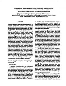
Figure 1: Inserting points one-by-one
This algorithm repeatedly adds one vertex at a time and re-triangulates the affected triangles. The steps are outlined below 1) Start with a triangle large enough to contain all the input points. Since this is the only triangle it satisfies the Delaunay property. 2) A new vertex ‘P’ is added to the existing Delaunay triangulation as follows: i) Find the triangle which contains the new vertex P. Let the three points of the triangle be A,B,C. This can be done by starting from arbitrary triangle and moving in the direction of P. ii) Delete the triangle ABC and create three new triangles which have the vertices as ABP, BCP and CAP. iii) The edges of the old triangle ABC are inspected to verify that they still
Figure 2: Inserting a point into the triangulation. Dashed lines indicate edges that need to be inspected. (e) is the result of flipping the dotted edge inside the circle in (d).
Section II: A Corner table approach to incremental algorithm The Corner Table [1] provides a compact data structure to represent triangle meshes: A triangle mesh is defined by specifying the set G of its
vertices and a set T of its triangles. A triangle is defined by the IDs of the three vertices that it interpolates. The V-table stores the vertex indices of G in sets of three. Each of these set represents a triangle. The association of a vertex with a triangle is denoted as a corner. So a triangle can be represented by choosing its corresponding three corners. The three corners of a triangle are stored in clockwise order. Given this ordering and a corner we can get the previous or next corner. Every triangle has three neighbors. The corner table captures this information in the ‘O’ (opposite) table. For every corner ‘c’ the corner ‘o’ of the neighboring triangle opposite to corner ‘c’ is stored. We use the following notation for the corner table implementation: G[ ]: Stores vertex coordinates V[ ]:(V-table):Stores triplets of indices forming a triangle. The corresponding vertex coordinates of the triangle can be accessed by using these three indices into G. O[ ](O-table): Stores the opposite corner for every corner corresponding to V.
c.n: next corner in c.t c.o: opposite corner c.l: left neighboring corner (c.p.o) c.r: right neighboring corner (c.n.o) The 2 main steps of the incremental algorithm are: i) Finding the triangle containing the newly inserted point ii) Create new triangles trivially and flip the edges if required to satisfy the Delaunay circumcircle criteria. The corner table is very handy for the incremental Delaunay triangulation algorithm. The corner table provides an easy method to walk through the triangle mesh and access the connectivity information. We briefly discuss how to do the above two operations using the corner table. i) Finding the triangle containing the new inserted point (see figure 4) i)
Start from any arbitrary triangle. We need to reach triangle t1containing the point P which is to be inserted.(figure 4). ii) Make a line segment which starts inside triangle t0 and ends at P (red line shown in figure 4). Let this be denoted as ‘L’.
Figure 3: Corner Table operations
Using the V and O tables, given a corner, c, we can access (See figure 3): c.t: its triangle. c.v:its vertex c.p: previous corners in c.t
Figure 4: Traversing the triangle mesh using the corner table approach for locating the triangle containing the point to be inserted
iii) Find the edge of t0 which intersects the line segment ‘L’. Let ‘c’ be the corner opposite to this edge. iv) c=c.n (next corner) . v) if( g(v(c)).isLeftOf(L) ) . c=c.r; /*(o(n(c))) move to right triangle*/ else c=c.l;/*o(p(c)) move to left triangle*/ vi) Check if c.t contains the point P. If yes then we found the triangle containing P else repeat step v). ii) Create new triangles trivially and flip the edges if required to satisfy the Delaunay circumcircle criteria.
note that we have a zero area triangle with the circumcenter at the infinity. In such cases we first check if the points are collinear, if yes then we simply flip the corresponding original edge to remove the zero area triangle. In figure 6, the red edge needs to be flipped. Corner ‘c’ is opposite to this red edge. The neighboring corners are marked using the operations on corner table described earlier. The result of flipping the edge is shown in the right configuration. The locations of the old corners are shown as well.
Once we found the triangle (with corner ‘c’) containing the new point to be inserted we can make a trivial triangulation as shown in figure 5. Addition of this new vertex results in addition of 9 new corners. Instead of deleting the old corners c,c.p and c.n we re-use them for one of the new triangles as shown in figure 5.
Figure 6: Flipping an edge using the corner table operators. The V-table and O-table are updated as show in the figure
Section III: Improvements incremental algorithm
Figure 5: Inserting a point in an existing triangle. Three new triangles are added and the old triangle is deleted. The Vtable and O-table are updated as show in the figure. The two new sets of corners are c1, c1.n, c1.p and c2, c2.n, c2.p.
The newly added triangles may not be Delaunay so we check the edges opposite to corners c1, c and c2. Flipping the edge in the corner table can also be done by patching the existing corners instead of adding new corners which will be highly inefficient (because deleting a corner is very costly). If the point happens to be on the edge (which means three points are collinear) we
to
the
The incremental algorithm described above spends a lot of time in locating the triangle containing the new point to be inserted. We propose a simple uniform grid based scheme which improves upon the incremental algorithm by speeding up the step of finding the triangle containing the new point to be inserted. Instead of using additional CPU memory we take advantage of modern graphics processors capability to render triangles efficiently and use the Video Frame Buffer for the uniform grid. This can be achieved as follows: i) Assign a different color to each triangle in the current set (see figure 7)
ii) When we want to find the triangle containing the point to be newly inserted we simply ask for its corresponding color in the frame buffer. Based on the color information we read we can directly get the triangle which contains the point. iii) There is a risk that this may not be the correct triangle containing the point if there are so many points in the data set that a pixel might actually correspond to multiple triangles. We can work around this by checking if the point is indeed inside the triangle. If the geometry test approves that the point is inside the triangle we are done. Otherwise we adopt the earlier strategy of traversing the triangle mesh using the corner table approach described earlier. Even if this step is required it is better than the naïve incremental algorithm which picks the starting triangle randomly because we have a good starting triangle to begin with which is close to the actual triangle containing the point.
r=(i&0xff0000)>>16 g=(i&0x00ff00)>>8 b=(i&0x0000ff)>>0 where ‘i’ is triangle number. Since each of r,g,b can have values from 0 to 255 we can represent 255*255*255 triangles using this color scheme. We can increase this range further by using the alpha color component ‘a’ in addition to r,g,b. 2) Instead of rendering all triangles after each insertion we limit ourselves to rendering only the affected area. 3) The circumcenters computed while checking for the Delaunay property are retained as these will be useful for computing the Voronoi Diagram which is the dual of the Delaunay triangulation. 4) The three vertices of the initial triangle which encompasses all the points are inserted in the end of the G[] table so that we do not have to compact the array later when we remove the triangles containing any of these three vertices. We still need to compact the V[] table representing corners when we remove the triangles which have any of the three vertices from the initial triangle. This can be done in linear time.
Section IV: Computing the Voronoi diagram for the point set.
Figure 7: Finding the triangle based on coloring scheme. Since the point P is colored red we know its triangle in constant time.
Some notes about the implementation: 1) Figure 7 shows the basic idea of painting the triangles in different color. We now show how to do this programmatically to represent large number of triangles. The r,g,b coloring scheme for painting the each triangle in different color is achieved as shown below (here >> is the right sift operator in C language):
The Voronoi diagram for a point set S is the partition of the plane which associates a region V(p) with each point p in S in such a way that all points in V(p) are closer to p than to any other point in S. The Delaunay triangulation and the Voronoi diagram are duals of each other. To generate the Voronoi region for a point, simply join the circumcenters of the triangles which the vertex is part of in clockwise or anti-clockwise order as shown in figure 7.
Section V: Results
Figure 8: The red line joins the circumcenters of the triangles which is the vertex is part of. The enclosing region inside the red loop is the vornoi region for the vertex V.
To display the Voronoi diagram of a all the points in the set using the corner table we use the following loop for each corner c { CC= circumcenter of c.t if(c.o==-1){ P=midpoint(G[V[c.p]], G[V[c.n]]); vec=(P-CC).scaled(Infinity); if( G[V[c]].IsLeftOf(G[V[n(i)]],G[V[p(i)]]) != CC.IsLeftOf(G[V[n(i)]],G[V[p(i)]]) ) drawline(CC,CC+ vec); else drawline(CC,CC-vec); } else if(c