we have △abc ∈ T ′. Suppose we remove all sites other than a, b, c, and then generate a discrete Voronoi diagram D′ = D({a, b, c}). Note that those grid ...
Computing Two-dimensional Delaunay Triangulation Using Graphics Hardware Guodong Rong, Tiow-Seng Tan, Thanh-Tung Cao, Stephanus ∗ School of Computing National University of Singapore
Abstract This paper presents a novel approach to compute, for a given point set S in R2 , its Delaunay triangulation T (S). Though prior work mentions the possibility of using the graphics processing unit (GPU) to compute Delaunay triangulations, no known implementation and performance have been reported. Our work uncovers various challenges in the use of GPU for such a purpose. In practice, our approach exploits the GPU to assist in the computation of a triangulation T ′ of S that is a good approximation to T (S). From that, the approach employs the CPU to transform T ′ to T (S). As a major part of the total work is done by the GPU with parallel computing capability, it is a fast and practical approach, particularly for a large number of points (millions with the current state-of-the-art GPU). For such cases, our current implementation can run up to 53% faster on a Core2 Duo machine when compared to Triangle, the well-known fastest Delaunay triangulation implementation. CR Categories: I.3.5 [Computer Graphics]: Computational Geometry and Object Modeling—Geometric algorithms; I.3.1 [Computer Graphics]: Hardware Architecture—Graphics processors Keywords: Voronoi diagram, GPGPU, computational geometry, graphics hardware
1
Introduction
The Delaunay triangulation T (S) for a set of points S is a useful geometric structure that has applications in various areas of science and technology [Fortune 1992]. In games and interactive applications, T (S) appears in the study of terrain rendering [Kang et al. 2006], path-finding [Lanctot et al. 2006], etc. Previous work on the use of modern graphics hardware computes the discrete Voronoi diagram D(S) of S, a structure that is related to T (S), and this work (for example, Hoff III et al. [1999]) mentions the possibility of obtaining T (S) from D(S). However, no known implementation and performance have been reported. We present such an effort here and realize that such a task is non-trivial. Let us first define the discrete Voronoi diagram and Delaunay triangulation so that we can discuss specifically the computational challenges of deriving the latter from the former. Let Ω be a connected region in R2 . Let S = {s1 , s2 , . . . , sn } be a set of n points in ∗ Emails: { rongguod | tants | caothanh | stephanu}@comp.nus.edu.sg. Project webpage: http://www.comp.nus.edu.sg/∼tants/delaunay.html
Ω. We use ||p − q|| to denote the Euclidean distance between two points p and q. For si ∈ S, we define: R(S; si ) = {p ∈ Ω : ||p − si || < ||p − sj ||, sj ∈ Ω, sj 6= si }. In other words, R(S; si ) is the set of points nearer to si than to any other point in S. The region Ω is partitioned into R(S; s1 ), R(S; s2 ), . . . , R(S; sn ) and their boundaries. This partition is called the Voronoi diagram of S, denoted by V(S). The elements of S are also called sites of this Voronoi diagram. R(S; si ) is called the Voronoi region of si . The line segments shared by the boundaries of two Voronoi regions are called Voronoi edges, and the points shared by the boundaries of three or more Voronoi regions are called Voronoi vertices. The discrete version of the Voronoi diagram V(S) is defined as follows. Let L be the set of all the integer grid points in Ω, i.e. L = Ω ∩ Z2 . For each (j, k) ∈ L, we define l(j, k) = i if (j, k) ∈ R(S; si ), that is, l(j, k) represents the ordinal number of the site whose Voronoi region contains the grid point (j, k). If the point (j, k) is at equal distance from two or more sites, we assign the minimum (or arbitrary) ordinal number from among these sites. The discrete Voronoi region for the site si is defined as D(S; si ) = {(j, k) ∈ L : l(j, k) = i}. Thus, L is partitioned into discrete Voronoi regions. They are collectively called the discrete Voronoi diagram, D(S). The Delaunay graph of S, denoted as T (S), is a plane, dual graph of V(S). In other words, the nodes of T (S) are the sites in S, so there is one node corresponding to each Voronoi region. There is an edge si sj if and only if R(S; si ) and R(S; sj ) share a Voronoi edge. So the edges in T (S) one-to-one correspond to the Voronoi edges in V(S). As a result, the faces of T (S) also one-to-one correspond to the Voronoi vertices in V(S). In the degenerate case with m ≥ 4 co-circular points in S generating a Voronoi vertex, the corresponding face in T (S) is a polygon of m sides. When Ω = R2 and when there is no degenerate case, T (S) is a triangulation, which is a plane graph having each face, other than the exterior face, a triangle. The Delaunay graph under this case is also called the Delaunay triangulation. For our work, we have Ω = R2 and we want to output a triangulation T (S). When there are degenerate cases, the output is a super-graph of T (S). With modern graphics processing units (GPUs), one can efficiently compute D(S) [Hoff III et al. 1999; Rong and Tan 2006]. Though T (S) can be derived from V(S) quite straightforwardly, it is nontrivial to do the same from D(S). We give here just two reasons. First, the adjacency relation between Voronoi regions in V(S) may not be the same as that in D(S); see Figure 1. Second, Voronoi regions D(S; si ) in D(S) may not be one connected component; see Figure 2. For both reasons, V(S) and D(S) do not have the same topology, and the dual graph of D(S) is not our required triangulation T (S). Thus, special processing needs to be incorporated in order to still derive efficiently T (S) from D(S). Besides, there are also challenges due to limited texture size and computational precision of D(S) to consider. The details are provided in later sections. Our work here overcomes the above challenges. The main contribution is a novel approach combining the power of the GPU and CPU to compute the Delaunay triangulation for a given point set S in R2 . Our implementation shows that the approach performs well, particularly for a large number of points. For such cases, it
and they will be clear when we discuss our proposed algorithm. We note that the GPU approach of Yamamoto [2004] may produce outputs with topological and numerical errors.
Figure 1: The red and blue Voronoi regions should be adjacent to each other in V(S), but are separated by the yellow and green regions in D(S). Dashed lines are the Voronoi edges in V(S). can outperform the best known Delaunay triangulation implementation called Triangle [Shewchuk 1996]. Note that Triangle is a CPU-based program. This paper is organized as follows. Section 2 reviews the previous work. Section 3 gives an overview of our new algorithm. The details of all the steps are discussed in Section 4. Section 5 provides the correctness proof of our algorithm. Experimental results are presented in Section 6. Finally, Section 7 concludes the paper.
2
Related Work
The Delaunay triangulation is an old but important concept in computational geometry. There are many algorithms developed for the CPU to efficiently compute Delaunay triangulations; see surveys [Aurenhammer 1991; Fortune 1992; Su and Drysdale 1995]. Among these, three algorithms are most commonly used: divideand-conquer, plane-sweep and randomized incremental.
There are generally two approaches in using the GPU for general purpose computations. One approach uses the many small processors in the GPU separately as the processors in a parallel machine, and uses the position of the pixels only as memory addresses. In this approach, the GPU is used in a fashion similar to the traditional parallel machines and can solve problems defined in continuous space. The other approach performs computation directly on textures. Such computation includes information of the positions of the pixels, and often utilizes the communication among pixels. This maps well to the architecture of the GPU. However, it generally is more suitable to solve problems defined in discrete/digital space. Our work here uses the GPU primarily with the flavor of the second approach, but solves (with the help of the CPU) a geometry problem defined in continuous space.
3
Algorithm Overview
The idea of our algorithm is straightforward: we map our set of sites S to a texture, compute the discrete Voronoi diagram D(S ′ ) where |S ′ | ≤ |S| and the sites in S ′ are on grid points, use it to derive a triangulation T ′ (S ′ ) that is close to our Delaunay triangulation T (S), and then repair and subsequently flip edges to obtain T (S). There are two major design decisions as discussed in the next two paragraphs. In the discussion, the grid points are the pixels in the texture, and each site has a unique color which is also the color of the Voronoi region containing the site. The color of a pixel is the color of the Voronoi region containing the center of this pixel.
The divide-and-conquer algorithm recursively divides a set of sites into two smaller sets, until a set is small enough to compute its Delaunay triangulation in constant time. Then, it gradually merges two small Delaunay triangulations into a bigger one, until all are merged into one mesh, forming the resulting triangulation. The plane-sweep algorithm uses a sweeping line to sweep from left to right to gradually build the mesh. Each time the line touches a site, or a circle passes three sites, the mesh is updated accordingly. This algorithm is first proposed to compute Voronoi diagrams, but is also applicable to Delaunay triangulations. The randomized incremental algorithm starts from a big triangle bounding all input sites, and then adds the sites one by one, in a random order. Each time a new site is added, the mesh is updated to maintain it being a Delaunay triangulation.
In generating a triangulation from a Voronoi diagram, we could either generate edges or triangles for the triangulation. From D(S ′ ), an edge of T ′ (S ′ ) can be derived from each grid point which has neighboring grid points belonging to one other Voronoi region, i.e. of a different color. In this way, an edge of T ′ (S ′ ) may be derived from many grid points, and the algorithm would need to remove duplicate edges. It is time-consuming to check duplicates and thus the alternative of computing triangles for T ′ (S ′ ) is adopted: a corner (other than those on the boundary of the texture) is shared by four grid points; a corner surrounded by grid points belonging to exactly three Voronoi regions (i.e. three different colors) generates one triangle, and similarly, one surrounded by grid points belonging to four Voronoi regions generates two triangles.
All three algorithms have the same expected time complexity of O(n log n) where n is the number of input sites. However, this does not mean that all run with the same efficiency in practice. Shewchuk [1996] implements all three algorithms in his Triangle package. His experience is that the divide-and-conquer algorithm is the fastest, and the randomized incremental slowest. We note that Triangle is the fastest program known to compute 2D Delaunay triangulations. This award-winning program has been optimized for more than ten years to have efficient memory management and robust geometry computations.
The point set S is mapped via a function M to S ′ . The measure of distance between a′ and b′ in S ′ (in the computation of D(S ′ )) could be defined as ||a′ − b′ || = ||a − b|| where a′ = M (a) and b′ = M (b). This approach can generate triangles with orientation not consistent to the Voronoi vertices, and can generate crossing edges. It thus needs expensive computation to validate each triangle generated. To avoid doing so, our approach adopts ||a′ − b′ || as the usual Euclidean distance between a′ and b′ . We show (in a later section) that this method does not generate duplicate and overlapping triangles, and the orientation of triangles are consistently counterclockwise.
Though there are numerous algorithms using the CPU to compute Delaunay triangulations, there is no known exact algorithm that capitalizes on the parallel computing capability of the GPU. At a quick glance, it is easy to compute Delaunay triangulations from those algorithms that compute discrete Voronoi diagrams [Hoff III et al. 1999]. Our work here uncovers numerous challenges that need to be overcome in order to transform discrete Voronoi diagrams to Delaunay triangulations in continuous space, and to outperform the best implementation of 2D Delaunay triangulations, Triangle. Some of these challenges are mentioned in the previous section,
The algorithm consists of the following ten steps where GPU steps are prefixed with G and CPU with C: ——————————————————————————– Step G1. Write the input sites S (in continuous space) into a texture (discrete space) with surviving sites denoted as S ′ ; Step G2. Compute the discrete Voronoi diagram D(S ′ ) using the jump flooding algorithm;
Step G3. Re-assign, if needed, each island to a Voronoi region that is connected to a site; Step G4. Find Voronoi vertices that are corners surrounded by three or four Voronoi regions; Step G5. Chain up Voronoi vertices within each row in the texture; Step G6. Construct one or two triangles for T ′ (S ′ ) from each Voronoi vertex; Step C1. Complete the construction of T ′ (S ′ ) with triangles around the convex hull of S ′ ; Step C2. Shift each site s′ ∈ S ′ in T ′ (S ′ ) to its respective position in S to result in a triangulation T ′ (S ′′ ) where S ′′ ⊆ S;
Figure 2: Corners v0 and v1 (incident by an island) generate two triangles that cross with each other.
Step C3. Insert each point in S − S ′′ into T ′ (S ′′ ) resulting in a triangulation T ′ (S); and finally Step C4. Flip edges in T ′ (S) to result in T (S) as required. ——————————————————————————–
4
Algorithm Details
This section details each step of our proposed algorithm.
4.1
v0 v1
Figure 3: A small portion of the Voronoi diagram is shown. Corners v0 and v1 (incident by an island) both generate the same triangle with red, blue and green sites.
GPU Steps
The purpose of the GPU steps is to compute a mesh that will be passed on to the CPU to complete as T ′ (S ′ ). G1 to G5 are carried out using shading programs in Cg [Mark et al. 2003], and G6 using CUDA [NVIDIA 2007] that enables parallel construction of triangles for the mesh. Step G1 – Write sites into texture
We scale the continuous space such that all sites can fit into our chosen texture (discrete space), and then render these sites into the texture. Note first that due to the resolution of the texture and the distribution of the sites, there may be two or more sites mapped to the same pixel. Only one of these sites is written at that pixel, and the rest thus become missing sites, and will be inserted to be a part of the triangulation in Step C3. Note second that we use half-float format for the texture to represent precisely integers between -2048 and 2047. This matches the largest texture size of 4096×4096 in currently available graphics cards. We should switch to texture of integer format when Cg 2.0 becomes available. Step G2 – Compute Voronoi diagram
With the texture of size m × m storing some sites, there are various ways to generate the discrete Voronoi diagram [Hoff III et al. 1999; Denny 2003; Rong and Tan 2006; Fischer and Gotsman 2006]. The na¨ıve approach of standard flooding can propagate information √ of a site step-by-step radically but it takes time proportional to 2m. We choose the better propagation approach of jump flooding, in particular, 1+JFA [Rong and Tan 2007] to compute the discrete Voronoi diagram. It takes time proportional to log m. We note that 1+JFA does not compute the exact discrete Voronoi diagram. The possible errors (on a few pixels) have little chance to alter the topology of the Voronoi diagram [Rong and Tan 2006]. This thus does not have adverse effects on the correctness of the algorithm. Step G3 – Remove islands
As shown in Figure 2, a Voronoi region of a site in the discrete Voronoi diagram may contain more than one connected region due
to the discrete nature of the texture. We call all those connected components not containing the site islands. Their presence can complicate the identification of usable Voronoi vertices (in the next step). Involving them in the identification of Voronoi vertices as in Figures 2 and 3 can result in crossing edges and duplicate triangles in T ′ (S ′ ). We discover a pixel as a part of an island as follows. For a pixel p belonging to the Voronoi region of a site s, we build a coordinate system with the origin at p and is aligned with the texture. If s is in the first quadrant, we examine the three neighbors of p at (1, 0), (1, 1) and (0, 1). If all these three neighbors have colors different from p, we say p is in an island. We define similarly when s is in the other three quadrants. If s is on one of the axes, we only check the neighbor next to p and between p and s. For example, if s is on the positive x-axis, we only check the neighbor at (1, 0). If this neighbor has a color different from that of p, we say p is in an island. For a pixel in an island, we replace the color of the pixel by the color of the closest site other than its original one. The removal of one pixel that is in an island can expose other pixels to be in islands. The operation of removing these pixels is then repeated until no new ones are found. The OpenGL extension GL ARB occlusion query is useful in detecting if any pixels in islands are removed and the process must be continued. In practice, a small number (less than 5) of iterations are sufficient. Step G4 – Locate Voronoi Vertices
Each pixel has four corners. Excluding corners (of pixels) along the boundary of the texture, each corner is incident by four pixels. A corner is defined as a Voronoi vertex if its four incident pixels are of three or four different colors, but with an exception. The exception is the case of three different colors where the two same color pixels are diagonally opposite (see Figure 4). In these cases, the two same color pixels are actually 8-connected, and they prevent the other two pixels of different colors from being adjacent. Respecting this topology, we do not classify such a corner as a Voronoi vertex. In the computation, the status (of being a Voronoi vertex or otherwise) of a corner is identified and recorded at (or owned by) the lower left pixel incident to the corner.
2
1
2
1
3
4
3
4
(a)
(b)
Figure 4: Three-color corners not identified as Voronoi vertices.
Step G5 – Chain up Voronoi Vertices
With the texture recording the Voronoi vertices in some of its pixels, for each row, this step performs a parallel prefix computation [Blelloch 1990] to record for each pixel the nearest Voronoi vertex to its right. In the process, we can also compute the total number of triangles to be generated from each row of Voronoi vertices, and the total number of triangles accumulatively for the rows. With these, we can “jump” over all the pixels which are not Voronoi vertices in the next step to generate triangles. Such a scheme of jumping is particularly useful to support using a texture with a large resolution while maintaining the computation time proportional to the size of the output, which is the number of triangles. Step G6 – Construct a Triangle Mesh
The result of Step G5 stored in an OpenGL texture is read into a pixel buffer object to allow CUDA to construct triangles in parallel. Reading a big texture takes time. With asynchronous readback possible with glReadPixels in OpenGL, we use that time to perform other bookkeeping tasks. One such activity is to derive a list of vertex coordinates in integer format from the input in double format. This list is used in Step C2 for shifting sites. Note that this Step G6 could not be done well with Cg as is the case of Step G1 to Step G5, since we need scatter operations that are only available in CUDA. Also, Step G1 to Step G5 do not perform well when implemented with CUDA since they map naturally to the parallel computation using shader programs. To construct the mesh, we use many parallel processes in CUDA, each of which handles one row of data in our texture. With the information on the number of triangles to be generated from Step G5, we can pre-allocate memory to enable processes to concurrently insert triangles into the mesh. For each pixel recording a Voronoi vertex due to three colors, a triangle is formed with the three sites represented by these colors. Similarly, for a Voronoi vertex due to four colors, two triangles are formed by the corresponding four sites. Note that CUDA running on the NVIDIA GeForce 8800 GTX does not support atomic operations. As such, updating the list of triangles incident to each site (which is used to link up adjacent triangles) cannot be performed in parallel. This results in a slight penalty on the computation time.
4.2
CPU Steps
Data stored in the texture due to the GPU steps is no longer needed, except for pixels on the boundary of the texture. These are read in parallel by CUDA into an array and copied to the main CPU memory for Step C1. Step C1 – Fix Convex Hull
Because some Voronoi vertices may lie outside the texture, their corresponding triangles were not generated in Step G6. In some cases, the absence of these triangles may split the mesh into several disconnected parts; see Figure 5. In this step, we traverse, in
Figure 5: Missing triangles due to Voronoi vertices lying outside the texture. The five triangles with one or more white dashed edges are missing. The mesh is separated into two disconnected parts.
clockwise order, along the boundary of the texture, starting from the leftmost pixel that belongs to the highest site, to discover those sites whose Voronoi regions occupy the boundary of the texture. We push the first two sites found into a stack. From the third site on, we push the new site found to the stack and then check the topmost three sites si , si−1 , si−2 in the stack. If they are in counterclockwise order, it means that there is a missing triangle. A new triangle si si−1 si−2 is inserted into the mesh, si−1 is removed from the stack, and the process is repeated until the topmost three sites are not in counterclockwise order (similar to Graham’s scan algorithm [1972]). The resulting mesh is T ′ (S ′ ). Step C2 – Shift Sites
This step shifts each site at s′ in the discrete space back to their original position at s in continuous space to compute T ′ (S ′′ ) where S ′′ ⊆ S. We handle this in three cases where F (s′ ) denotes the triangle fan of s′ : Case 1: s is inside F (s′ ). Going through triangles in F (s′ ), we can determine that s lies inside a triangle in F (s′ ) through the counterclockwise test. Also with the same test, we determine whether s′ can be simply moved to s without creating crossing edges in the mesh. If so, we are done (Figure 6(a)). Otherwise, we insert s into the mesh by creating a triangle, deleting edges incident to s′ , and triangulating the resulting polygonal region or curve (shown in green in Figures 6(b) and 6(c)). Case 2: s is in a triangle not inside F (s′ ). By stepping from triangle to triangle starting with those in F (s′ ), we can determine the triangle in the mesh containing s. Insert s to create three triangles (or four triangles if s is on an edge), delete the edges incident to s′ , and triangulate the resulting polygonal region or curve (shown in green in Figures 6(d) and 6(e)). Case 3: s is outside the mesh. This is the case when the stepping from triangle to triangle fails to locate s in any triangle. If s′ is not on the boundary of the convex hull, we delete edges incident to s′ , triangulate the resulting polygon (shown in green in Figure 6(f)), insert s, and triangulate around the boundary of the (new) convex hull. Otherwise, s′ is on the boundary of the convex hull. We either have to move s′ to s without any further processing (as in Figure 6(g)), or repair the convex hull by deleting edges incident to s′ and inserting s on the boundary of the convex hull (as in Figure 6(h)). Note that counterclockwise tests are often used in the process. Step G6 while generating triangles can pre-compute and record the outcomes of some of these tests. This is an optimization that improves the running time significantly. Not all such tests can be recorded as there are triangles generated in Step C1 that are not by Step G6, and there are triangles (after shifting some of their vertices) that CUDA (which currently supports only float format as
(a)
(b)
(c)
Figure 7: Two colors alternate around a corner. Flooding does not generate such a configuration.
(d)
(f)
(e)
(g)
(h)
Figure 6: Shifting sites: (a)-(c) are Case 1, (d)-(e) Case 2, and (f)-(h) Case 3. s′ is represented by the black point and s by the red point. The solid lines show the triangles before shifting while the dotted lines show the triangles after shifting. The green lines indicate the polygonal region or curve that are to be triangulated.
compared to the input data that is in double format) cannot perform reasonably robust tests due to insufficient precision. Step C3 – Insert Missing Sites
This step handles missing sites due to Step G1. Suppose that s and t are mapped to the same pixel in Step G1, and s is recorded as s′ , then t becomes a missing site. To insert t into the mesh, we start from the triangle fan of s to locate the position of t, which is either inside a triangle of the mesh, or falling on an edge of the mesh, or outside the mesh. The remaining processing of inserting t into the mesh is straightforwardly a subdivision of a triangle into three triangles, two triangles into four triangles, or fixing the convex hull when t lies outside the old convex hull. The resulting mesh is a triangulation T ′ (S). Step C4 – Flip Edges
T ′ (S) may not be a Delaunay triangulation for various reasons. First, a low-resolution texture may cause topology change (as shown in Figure 1). Second, in Step G6, when there are four colors around a Voronoi vertex, we generate two triangles arbitrarily. Third, Steps C1 to C3 also arbitrarily re-triangulate polygons or curves in the mesh. In this step, we traverse all the triangles in the mesh one by one. For an edge ab of ∆abc, it passes the empty circle property if ab is a convex hull edge, or if the other triangle ∆adb incident to ab is such that d lies outside the circumcircle of ∆abc. If ab fails the empty circle property, an edge-flip occurs to replace ∆abc and ∆adb by triangles ∆adc and ∆cdb, and new tests apply to edges of these new triangles. This step is performed until all edges pass the empty circle property. The resulting mesh is the required Delaunay triangulation T (S).
5
Proof of Correctness
This section proves that our algorithm computes correctly the Delaunay triangulation T (S) of S. The main challenge is to show that we can derive from the discrete Voronoi diagram D(S ′ ) a mesh in Step G6 that we can augment with more triangles into a triangulation in Step C1.
Consider using the standard flooding to generate a Voronoi diagram. A corner, incident by four pixels, cannot have two colors alternate around the corner (see Figure 7); otherwise, one of these pixels would lie on the wrong side of the perpendicular bisector of the sites having these colors. In the following properties, we adopt 8-connectedness where two pixels that are 8-connected at a corner is interpreted as connected through a tiny neck at the corner. For example, the pixels marked 2 and 4 in Figure 4(a) are considered connected to each other. Property 1 Each Voronoi region generated by the standard flooding is simply-connected. Proof. Each Voronoi region generated by the standard flooding is connected by induction: the site whose information first reaches a pixel is the nearest site to that pixel, so a pixel never changes its color (i.e. nearest site) once assigned; each pixel is connected to a neighbor having the same color, which is in turn inductively connected to the nearest site to the pixel. If a region D(S ′ ; si ) is not simple, then at least one other region, say D(S ′ ; sj ), appears as a hole in D(S ′ ; si ). Consider the line l passing through si and sj , it is clear that the part of l closer to sj than si and intersects D(S ′ ; si ) cannot be part of D(S ′ ; si ). So, there is no such hole D(S ′ ; sj ) inside D(S ′ ; si ). � Instead of the standard flooding, our algorithm uses the more efficient jump flooding algorithm (JFA) [Rong and Tan 2006]. This is at the expense of two potential problems. First, a Voronoi region generated by the JFA is not necessarily simply-connected. One reason is that there can be one D(S ′ ; si ) that is disconnected into one component containing si and the others as islands. Islands are removed by Step G3, and thus no longer an issue. Another possibility is the existence of a D(S ′ ; sj ) appearing as a hole in D(S ′ ; si ). Such a scenario has not been detected in our extensive experimentations. Nevertheless, we can perform some additional passes of flooding with the step length of 1, utilizing GL ARB occlusion query, to remove holes. Second, JFA may not generate correct D(S ′ ; si ) for all si . There are however only a few pixels with errors, and these errors are at Voronoi vertices in most cases [Rong and Tan 2006]. All these do not change the topology of the discrete Voronoi diagram, and are thus not issues for our algorithm. We can thus assume Property 1 and Figure 7 hold for our algorithm. In the following properties, triangle refers to one that was generated during Step G6. Let the mesh generated at the completion of Step G6 be T ′ . Property 2 All triangles in T ′ are consistent in orientation. Proof. We first consider three sites, a, b and c whose Voronoi regions are incident, in counterclockwise order, at a corner v. Then, we have △abc ∈ T ′ . Suppose we remove all sites other than a, b, c, and then generate a discrete Voronoi diagram D′ = D({a, b, c}). Note that those grid points colored by the colors of a, b and c, respectively, in D(S ′ ) remain the same in D′ ; in particular, corner v is still incident by the same three colors in the same order. By joining a ray each from v to a, b and c, we read around the boundary of D′ (making D′ large enough) to note the order of the intersection
points a′ , b′ , c′ . Notice that all the three angles at v formed by the three rays are never larger than π; thus, a, b, c are in the same order as a′ , b′ , c′ . Suppose on the contrary that this order is clockwise, then D′ has a corner v ′ 6= v that is incident by alternate colors of a and b, or b and c, or c and a so that each of the three Voronoi regions can remain simply connected (as shown in Property 1) while able to reach v in counterclockwise order. Such a v ′ is impossible as explained in Figure 7. So, a, b, c are in counterclockwise order, as needed. Next, we consider four sites, a, b, c and d whose Voronoi regions are incident at a corner v in D(S ′ ). Viewing from v, we see that a, b, c and d are in the same order as their Voronoi regions incident at v; otherwise, for any three of them, we can use the argument in the previous paragraph to derive a contradiction. � Note that in the case of a corner incident by four colors, one of the two triangles generated by the algorithm may have zero area. This does not cause any problem in the final result, as such triangles are removed (flipped away) in Step C4. We thus ignore, for simplicity, the existence of such triangles in our argument. Property 3 No two edges of triangles in T ′ intersect. Additionally, no endpoint of any edge lies on another edge. Proof. Suppose on the contrary that a triangle with edge ac crosses another triangle with edge bd. Then, sites a, b, c, d form a convex polygon. Consider the discrete Voronoi diagram D′ = D({a, b, c, d}), which (as in the proof of Property 2) maintains grid ′ points colored by the colors of a, b, c and d. The dual graph D of ′ D is a complete graph K4 of four vertices as each site is a neighbor to the other three. We note that the only plane embedding of K4 is with three vertices incident to edges that bound a region that encloses the fourth vertex (K4 is the smallest non-outerplanar graph). ′ But, our D has a 4-gon as its outer region, and thus cannot be a ′ plane graph. This contradicts the fact that D is a plane graph as ′ each Voronoi region of D is simply connected (Property 1). The above argument, with minor adjustment, is also applicable to show that no endpoint of any edge lies on another edge. � Property 4 No two faces of triangles in T ′ overlap in area. Proof. Because of Property 3, there are only two ways for triangles to overlap in area: first, when the two triangles have the same set of three vertices, and second, when one triangle is completely enclosed by the other. The former means that there are duplicate triangles, say △abc. This means that in Step G6, there are two Voronoi vertices having colors of sites a, b and c around them. This leads to two of these three colors occurring alternatively around a corner, which is impossible as explained in Figure 7. Next, we consider the latter way of overlapping. Let triangle △xyc be enclosed in triangle △abd where x may be a, and y may be b. Among x, y, c, we can assume the extremal property that c is closest to d when x 6= a or y 6= b. So D(S ′ ) is such that D(S ′ ; c) appears as a hole in the union of D(S ′ ; a) and D(S ′ ; b). Now, consider the Voronoi diagram D′ = D′ ({a, b, c}). Grid points colored by the colors of the three sites in D(S ′ ) remain having the same colors in D′ . As a result, D′ has the Voronoi region D({a, b, c}; c) that is not connected or is enclosed by the other two regions. This is not possible as each Voronoi region for three sites must be connected and must appear on the boundary of a large enough D′ . � Property 5 Each edge in T ′ is shared by at most two triangles. Proof. This is immediate from the previous property as three or more triangles sharing an edge would result in triangles with overlaping areas. �
lbc lab b c a d e Boundary of texture
v
Figure 8: The edge de cannot exist and there is thus no holes in T ′ . Property 6 The union of all triangles in T ′ does not enclose a bounded region that is not part of T ′ . Proof. Suppose on the contrary that there exists such a bounded region, which is a polygon. Note that any polygon of three or more vertices has an ear. Suppose we have consecutive vertices a, b, c in counterclockwise order forming an ear. Let lab and lbc be the perpendicular bisectors of a, b and b, c, respectively, and they intersect at v. We consider two cases where v is or is not a Voronoi vertex; refer to Figure 8. First, if v is a Voronoi vertex, then v must be outside D(S ′ ); otherwise, we are done as ∆abc exists in T ′ . Figure 8 shows the bounded region where d is possibly c, and e is possibly a. Consider the Voronoi diagram D′ = D({a, b, c, d, e}). By the familiar argument as in the proofs of the above properties, it is clear that there cannot be an edge in T ′ that crosses from the half-space containing e defined by lab to that containing d defined by lbc . In other words, the assumption on the existence of a bounded region is incorrect. Second, if v is not a Voronoi vertex, then some points in ∆vbc ∩ lbc (or, in a similar case, ∆vab ∩ lab ) belong to Voronoi regions other than that of b and c (or, in a similar case, a and b). One such point v ′ is on a perpendicular bisector of two vertices of the polygon and is closer to these two vertices than v is to b (and c). We can thus employ an extremal property to find a v that is an intersection of two perpendicular bisectors of vertices of the polygon and v is indeed a Voronoi vertex. With these, we can adapt the argument in the previous paragraph to arrive at a contradiction. � Property 7 At the end of Step C1, T ′ (S ′ ) is a triangulation of S ′ . Proof. At the end of Step G6, T ′ is a mesh in most cases, with the exception that it may have more than one component (where an isolated site can be a component), or there may be pinch points at some vertices. If T ′ is one single component, the algorithm clearly completes T ′ to a triangulation. So, suppose it is otherwise. Then, there are two or more Voronoi regions that spread from one boundary to another boundary as shown in Figure 5. In such case, the algorithm going around the boundary of D(S ′ ) can connect in consecutive order one vertex of a component to a vertex of the other component. As such, the algorithm can link up all vertices of S ′ into a single component in T ′ (S ′ ). � Theorem 1 The proposed algorithm computes the Delaunay triangulation of S. Proof. From the above properties, we know that up to Step C1, we have a triangulation of S ′ . Step C2 shifts the set of sites so that it is now a subset of S while maintaining the mesh as a triangulation. Then, Step C3 includes all points of S into the triangulation constructed so far. Finally, Step C4 converts our triangulation to a Delaunay triangulation through edge-flip, and we are done. �
x
x
(a)
(b)
x
x
(c)
(d)
Figure 9: Experimental results
6
Experimental Results
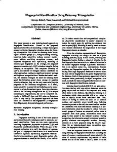
We have tested our algorithm on an Intel Core2 Duo 1.86 GHz PC with 2 GB DDR2 RAM and an NVIDIA GeForce 8800 GTX PCI-X with 768 MB DDR3 VRAM. Our program is developed using Microsoft Visual C++.NET 2005, and compiled with all optimization options enabled. The GPU programs are written and compiled with NVIDIA Cg 1.5 and NVIDIA CUDA 1.0. For the purpose of comparison, our program outputs Delaunay triangulations in the same data structure as that by the Triangle program, and uses the same robustness routine as Triangle [Shewchuk 1996]. We, however, have not implemented other useful features, such as incorporating constrained edges or augmenting the given sites with new vertices, available in Triangle. Running Time. On the whole, our algorithm (with still more optimization possible) running on uniformly distributed sites can achieve up to 53% improvement over Triangle. Figure 9(a) shows the comparison of the running time of Triangle and our algorithm for different texture resolutions. The ratio of the difference between the running time of Triangle and our program to the smaller running time of the two gives the percentage of improvement. Positive improvement means ours is faster than Triangle; see Figure 9(b). For a small number of sites, Triangle is faster than our program, as our program has certain overhead due to the use of the GPU computation. For a fixed texture resolution (such as 4096×4096 in Figure 9(c)), the computational time of the GPU, excluding Step G6, is relatively constant since these steps are almost independent of the total number of Voronoi sites. The timings of Step G6 and the CPU part of our algorithm increase with the increase in the number of Voronoi sites. Figure 9(c) when applied to other texture sizes also looks similar. Currently, those CPU steps, especially C2 to C4, still dominate the computational time. New features in the GPU such as
atomic operations may help to eventually realize some of them in the GPU, and thus further improve computational time. On the other hand, our algorithm does not perform as fast, though remains robust as Triangle, when running on an input with nonuniformly distributed sites such as the Gaussian, nearly co-circular, or nearly collinear cases. In the case of the Gaussian distribution, many sites are concentrated near the centroid of these sites. Thus, the algorithm has more missing sites to handle and cannot perform as efficiently as it can in the uniformly distributed case. Figure 9(d) shows that the algorithm performs up to 22% faster for Gaussian distribution of sites (as compared to 53% for uniformly distributed cases), using a texture of 4096×4096, but only slightly faster when using a texture of 2048×2048. As for co-circular or nearly collinear cases, there are even more missing sites to handle as the mapping of Step G1 results in most parts of the texture remain empty. As such, our algorithm behaves like the randomized incremental algorithm (but without any form of optimization) in constructing a Delaunay triangulation, thus it runs very slowly when compared to Triangle which uses a divide-and-conquer approach. Texture Resolution. The resolution of the texture is a parameter in our algorithm; it affects the running time of the CPU steps as shown in Figure 10. For a larger texture, Step C1 spends slightly more time to traverse along the boundary, while Step C3 has fewer missing sites to handle and Step C4 has fewer edges to flip. Increasing the texture resolution moves the problem closer to continuous space, and Step G6 thus computes a mesh closer to the required output and Steps C3 and C4 have less to do. On the other hand, Step C2 does not behave in a monotonic manner. With a larger texture, more sites are shifted straightforwardly as shown in Figure 6(a), but there are also more sites to be handled due to less missing sites. As such, the time needed for Step C2 can increase with the increase in the texture resolution.
on a single (inexpensive) machine. Thus, it may not be appropriate to compare our algorithm to the traditional parallel ones. On the other hand, there remains possible work to further improve our implementation. For example, one can consider the possibility of utilizing atomic operations in CUDA to better realize some parts that are currently performed by the CPU.
Acknowledgements
Figure 10: Timings on one million sites using different texture resolutions.
The authors would like to thank Herbert Edelsbrunner for contributing the major ideas in the proof of correction. They would also like to thank anonymous reviewers for their comments to improve the presentation of the paper. This research is supported by National University of Singapore under the grant R-252-000-254-112.
References Nevertheless, the total CPU time decreases with an increase in texture resolution. For our hardware configuration and as shown in Figure 9(b), we should use resolution of 4096×4096 for more than 600K sites, but smaller resolution otherwise. Examining carefully Figure 9(b) and also Figure 9(d), we notice the crossing pattern among the four curves of different texture sizes: as the number of sites increases, the algorithm should gradually switch to a larger texture size to remain efficient when compared to a pure CPU algorithm. This means that, assuming there is no limit on the texture size (and memory), our algorithm can possibly run well for very large data sets. More experiments should be conducted to ascertain this when larger texture sizes become available in the future. Memory Usage. The CPU memory needed for Triangle is about 80n bytes where n is the number of input sites. For our CPU computation, we need, besides the above amount, about 48n bytes more to keep track of vertices for shifting and a list of references to triangles incident to each site. Such additional CPU memory is used in linking up adjacent triangles sharing a site. Also, we need 384 MB each in the CPU and GPU for the 4096×4096 textures and pixel buffer objects. Specific to just the GPU, we need about 72n bytes more to keep information on the triangles generated. With all these on our GPU with 768 MB of memory, our program can run on slightly more than five million sites. It is possible to reduce the amount of memory usage, and we are continuing to optimize our current implementation. On a side note, Step G6 requires the copying of an OpenGL texture to a pixel buffer object for CUDA to use. This results in a bigger memory footprint. Should it be possible to read OpenGL textures directly with CUDA, our program would run with a smaller memory footprint.
7
Concluding Remarks
In this paper, we propose a new algorithm to compute Delaunay triangulations in continuous space using the GPU and CPU together. Although previous researches use the GPU to compute discrete Voronoi diagrams, it is not a trivial task to derive a Delaunay triangulation in continuous space from a discrete Voronoi diagram. This work addresses all the problems and successfully implements an algorithm that can run faster than the best Delaunay triangulation program for a large number of uniformly distributed sites. We have also proven the correctness of our algorithm. This algorithm demonstrates a new direction in using the GPU (with the help of the CPU) to solve geometry problems in continuous space, and it serves to challenge investigations of such an approach on other geometry problems. Though the speedup is yet to be as exciting as that of the traditional parallel computation [Kohout et al. 2005], our approach here remains fundamentally sequential in that it runs
AURENHAMMER , F. 1991. Voronoi diagrams—a survey of a fundamental geometric data structure. ACM Computing Surveys 23, 3, 345–405. B LELLOCH , G. E. 1990. Prefix sums and their applications. Tech. Rep. CMU-CS-90-190, School of Computer Science, Carnegie Mellon University, Nov. D ENNY, M. O. 2003. Algorithmic geometry via graphics hardware. PhD thesis, Universit¨at des Saarlandes. F ISCHER , I., AND G OTSMAN , C. 2006. Fast approximation of high order Voronoi diagrams and distance transforms on the GPU. Journal of Graphics Tools 11, 4, 39–60. F ORTUNE , S. 1992. Voronoi diagrams and Delaunay triangulations. In Computing in Euclidean Geometry, D.-Z. Du and F. Hwang, Eds., vol. 1 of Lecture Notes Series on Computing. World Scientific, Singapore, 163–172. G RAHAM , R. L. 1972. An efficient algorithm for determining the convex hull of a finite planar set. Information Processing Letters 1, 4, 132–133. H OFF III, K. E., C ULVER , T., K EYSER , J., L IN , M., AND M ANOCHA , D. 1999. Fast computation of generalized Voronoi diagrams using graphics hardware. In Proceedings of ACM SIGGRAPH 99, ACM Press / ACM SIGGRAPH, New York, 277– 286. Computer Graphics Proceedings, Annual Conference Series, ACM. K ANG , D.-S., K IM , Y.-J., AND S HIN , B.-S. 2006. Efficient largescale terrain rendering method for real-world game simulation. In Edutainment, 597–605. ´ , J. 2005. Parallel KOHOUT, J., KOLINGEROV A´ , I., AND Zˇ ARA Delaunay triangulation in E 2 and E 3 for computers with shared memory. Parallel Computing 31, 5, 491–522. L ANCTOT, M., S UN , N. N. M., AND V ERBRUGGE , C. 2006. Path-finding for large scale multiplayer computer games. In Proceedings of the Second North American Game-On Conference. M ARK , W. R., G LANVILLE , R. S., A KELEY, K., AND K ILGARD , M. J. 2003. Cg: a system for programming graphics hardware in a C-like language. ACM Transactions on Graphics 22, 3, 896– 907. NVIDIA, 2007. NVIDIA CUDA compute unified device architecture programming guide, Jan. http://developer. nvidia.com/cuda.
RONG , G., AND TAN , T.-S. 2006. Jump flooding in GPU with applications to Voronoi diagram and distance transform. In Proceedings of the Symposium on Interactive 3D Graphics and Games, ACM Press, 109–116. RONG , G., AND TAN , T.-S. 2007. Variants of jump flooding algorithm for computing discrete Voronoi diagrams. In Proceedings of the 4th International Symposium on Voronoi Diagrams in Science and Engineering (ISVD’07), 176–181. S HEWCHUK , J. R. 1996. Triangle: Engineering a 2D quality mesh generator and Delaunay triangulator. In Applied Computational Geometry: Towards Geometric Engineering, M. C. Lin and D. Manocha, Eds., vol. 1148 of Lecture Notes in Computer Science. Springer-Verlag, 203–222. See also http://www. cs.cmu.edu/˜quake/triangle.html. S U , P., AND D RYSDALE , R. L. S. 1995. A comparison of sequential Delaunay triangulation algorithms. In Symposium on Computational Geometry, 61–70. YAMAMOTO , O. 2004. Fast computation of 3-dimensional convex hulls using graphics hardware. In Proceedings of International Symposium on Voronoi Diagrams in Science and Engineering, 179–190.