Remote Sens. 2015, 7, 1640-1666; doi:10.3390/rs70201640 OPEN ACCESS
remote sensing ISSN 2072-4292 www.mdpi.com/journal/remotesensing Article
An Improved Unmixing-Based Fusion Method: Potential Application to Remote Monitoring of Inland Waters Yulong Guo 1,†, Yunmei Li 1,2,*, Li Zhu 3,†, Ge Liu 1,†, Shuai Wang 1,† and Chenggong Du 1,† 1
2
3
†
Jiangsu Provincial Key Laboratory of Carbon and Nitrogen Cycle Processes and Pollution Control, Nanjing 210023, China; E-Mails:
[email protected] (G.Y.);
[email protected] (L.G.);
[email protected] (W.S.);
[email protected] (D.C.) Jiangsu Center for Collaborative Innovation in Geographical Information Resource Development and Application, Nanjing 210023, China Satellite Environment Application Center, Ministry of Environmental Protection, Beijing 100029, China; E-Mail:
[email protected] These authors contributed equally to this work.
* Author to whom correspondence should be addressed; E-Mail:
[email protected]; Tel.: +86-25-8589-8500. Academic Editors: Deepak Mishra and Prasad S. Thenkabail Received: 28 September 2014 / Accepted: 6 January 2015 / Published: 5 February 2015
Abstract: Although remote sensing technology has been widely used to monitor inland water bodies; the lack of suitable data with high spatial and spectral resolution has severely obstructed its practical development. The objective of this study is to improve the unmixing-based fusion (UBF) method to produce fused images that maintain both spectral and spatial information from the original images. Images from Environmental Satellite 1 (HJ1) and Medium Resolution Imaging Spectrometer (MERIS) were used in this study to validate the method. An improved UBF (IUBF) algorithm is established by selecting a proper HJ1-CCD image band for each MERIS band and thereafter applying an unsupervised classification method in each sliding window. Viewing in the visual sense—the radiance and the spectrum—the results show that the improved method effectively yields images with the spatial resolution of the HJ1-CCD image and the spectrum resolution of the MERIS image. When validated using two datasets; the ERGAS index (Relative Dimensionless Global Error) indicates that IUBF is more robust than UBF. Finally, the fused data were applied to evaluate the chlorophyll a concentrations (Cchla) in Taihu Lake. The result shows that the Cchla map obtained by IUBF fusion captures more detailed information than that of MERIS.
Remote Sens. 2015, 7
1641
Keywords: image fusion; unmixing-based fusion method; inland case 2 water; remote monitoring
1. Introduction Inland waters play an important role in ecosystems. However, with increasing human activities over the past several decades, pollution of inland water has become a major problem, causing diseases worldwide and accounting for the deaths of more than 14,000 people globally each day [1]. So, effective monitoring of inland water is desired. However, traditional monitoring methods are time-consuming, labor-intensive, and -costly. In recent years, numerous studies have been focused on remote monitoring of water quality of inland waters based on various satellite image data [2–6] with wide spatial and temporal coverage [7]. To successfully monitor in land waters remotely, more and higher-level requirements for spatial and spectral resolutions of satellite image data have emerged. Because inland case 2 water (The global waters are classified into case 1 and case 2 waters. Case 1 waters are those waters whose optical properties are determined primarily by phytoplankton and related colored dissolved organic matter (CDOM). Case 2 waters are whose optical properties are significantly influenced by other constituents such as mineral particles, CDOM, or microbubbles [8,9]) is always changeable, its optical properties are more complicated than those of ocean water (most ocean water belongs to case 1 waters), Retrieval models for inland water constituents always need more bands [10,11]. Odermatt et al. [12] have provided a comprehensive overview of water constituent retrieval algorithms and have found that the regression models for Landsat-7 Enhanced Thematic Mapper Plus (ETM+) and Landsat-5 Thematic Mapper (TM) images had a weaker performance compared with the NIR-red algorithms using MERIS and Moderate-resolution Imaging Spectroradiometer (MODIS) images. Moreover, high spatial resolution of remote sensing data is also required to detect changes in the distribution of complex coastal water and inland water [13–17]. However, high spectral resolution and high spatial resolution cannot be obtained from the same sensor due to hardware limitations. For instance, although the MODIS and Sea-viewing Wide Field-of-view Sensor (SeaWiFS) both have special water-colour wavelengths and have been widely used in ocean and near-shore remote colour sensing [18–21], they are rarely applied for inland water monitoring. One of the reasons is that their 1-km spatial resolution is not sufficient for inland waters. Other satellite sensors, such as Landsat TM and ETM+, have a much higher spatial resolution (30 m), but their band settings are not appropriate for retrieving water component constituents because they have fewer and wider bands than the previously described satellites. MERIS data are an excellent data source for coastal water monitoring [22,23], but a recent study has indicated that the current global chlorophyll concentration is underestimated due to its coarse spatial resolution [24]. Therefore, a proper image fusion method is needed for inland case 2 water monitoring to combine spatial resolution and spectral resolution advantages of different remote sensors. The normally used image fusion methods, such as principal component analysis-based methods, transform domain-based methods and intensity-hue-saturation fusion techniques, etc., mainly focus on pan and multispectral image fusion. Thus, the problem common to these methods is colour distortion [25]. Tu et al. [26] studied the colour space of images and indicated that this distortion problem arises from the change in the
Remote Sens. 2015, 7
1642
information in transformed spaces during the fusion process. Meanwhile, bio-optical model based ocean colour satellite data merging methods [27–29] could yield high-quality normalised water-leaving radiance spectrums. However, the spatial resolution is neglected because the main purpose of those methods is to enhance spatial and temporal coverage of ocean colour products. Those methods are not suitable for remote inland water colour sensing. The objective of this study is to propose an image fusion algorithm to generate more appropriate image data for remote monitoring of optical complex inland case 2 waters. 2. Materials 2.1. Study Area The study area, Taihu Lake (Figure 1), located between Jiangsu and Zhejiang Provinces (China), is a large shallow inland lake with an area of approximately 2338 km2 and a mean depth of approximately 1.9 m [30]. The lake is suffering from water quality deterioration and also shows high turbidity in some areas due to a large quantity of sediment resuspension. These factors have led to the presence of complex water conditions in this water body.
Figure 1. Location of the study area. 2.2. Datasets The Environmental Satellite 1 (HJ1-CCD) image (relatively high spatial resolution image), and the MERIS image (low spatial resolution with higher spectral resolution) were used in this study.
Remote Sens. 2015, 7
1643
Considering the extreme changeability of the inland water, two simultaneous image datasets were selected (Table 1). To show the complex water conditions of the study area, the two datasets were acquired for August and October because algal blooms frequently appear in Taihu Lake during the summer and autumn [31,32]. Table 1. Information from two datasets. Dataset
Date
Image Data
Sensing Time Difference
Usage
#1
5 October 2010
HJ1-CCD image; MERIS image
6 min
Algorithm validation and parameter optimisation
#2
9 August 2010
HJ1-CCD image; MERIS image;
7 min
Algorithm application
The HJ1 A and B satellites were launched by China in September 2008. Both were optical satellites (i.e., HJ1A and HJ1B), and each of them was equipped with two CCD cameras (CCD1 and CCD2). The main characteristics of the HJ1-CCD image data are shown in Table 2 [33,34]. These data provide the potential for inland water monitoring due to the fine spatial resolution (30 m) and short revisit time (2 days). Geometric correction was carried out using ENVI software based on a reference TM image with exact geographical coordinates [30]. The corrected error for HJ1-CCD images is less than 1 pixel. Table 2. Main technical parameters of HJ1-CCD and MERIS. Specifications
HJ1-CCD
MERIS
Swath width(km) Altitude(km) Spatial resolution(m) Revisit time(days) Quantitative value(bit) Average Signal to noise ratio(dB)
360 750 30 2 8 ≥48
1150 800 1200/300 3 16 1650
Centre(nm)
Band setting
Width(nm)
Centre(nm)
Width(nm)
412.5
10 10 10 10
475
90
442.5 490 510
560
80
560
10
60
620 665 681.25
10 10 7.5
708.75 753.75
10 7.5
761.875 778.75 865
3.75 15 20
660
830
140
The MERIS sensor, launched on board ENVISAT in 2002, was designed for ocean colour observation, with a 300-m spatial resolution, 15 spectral bands and a 3-day revisit period. The MERIS full-resolution images were geometrically corrected, and the smile effect was removed using the BEAM
Remote Sens. 2015, 7
1644
software [35]. Because atmospheric correction might cause unexpected errors, to focus on the image fusion algorithms, the two images were only radiometrically calibrated to convert digital numbers of the images into top-of-atmosphere radiance (mW/m2/sr/nm) in dataset #1. The atmospheric correction is only applied in dataset #2 to estimate the concentration of chlorophyll a (Cchla). The detailed strategies of atmospheric correction and Cchla measurement are described elsewhere [3]. 3. Methods 3.1. The Unmixing-Based Fusion (UBF) Method The UBF method [36] is a good solution to downscale low resolution images. The basic idea of UBF algorithm is composite with the widely used unmixing applications: the abundances of each endmember are derived from the known high spatial resolution image. The endmembers are to be derived in the UBF method. The main advantage of UBF is that this method does not require a priori knowledge of the endmembers, and the fusion can maintain the relatively high spectral information of the low spatial-resolution image in the final result [37]. The UBF method has been successfully applied in vegetation dynamics [38–40], land-cover mapping [41] and coastal water monitoring [42], etc. The UBF method consists of the following four steps [36]: Step 1: The high spatial resolution image is used to identify the abundances of the image. This is done by classifying the high-resolution image into several unsupervised classes using the Iterative Self-Organising Data Analysis Techniques Algorithm (ISODATA). Step 2: Computing the proportions for each class that falls within the low spatial-resolution image pixels. Step 3: Unmixing the spectral behaviour of each class (i.e., endmember) according to the proportions and the spectral information provided by the low resolution sensor. Here, it is important to notice that in contrast to linear spectral unmixing, which is solved per pixel and for all bands at once, spatial unmixing is solved per pixel, per band, and for a given neighbourhood around the pixel that is being unmixed. The neighbourhood size needs to obtain enough equations to solve the unmixing problem. Step 4: Reconstructing the fused image by joining all of the low resolution pixels that have been spatially unmixed. Several problems occur when this method is applied to inland-water satellite images. First, the water body is always assigned as a lower radiance signal than other features and has even been treated as a “dark pixel” [43] due to its strong absorption. Therefore, a large area of water is usually assigned as only one class by the unsupervised classification method that results in the “unique endmember effect”, i.e., numerous pixels that should be identified by a MERIS pixel size belong to the same class. In that case, these various pixels would be calculated in the same numeric form (i.e., all equal to the specific endmembers of the corresponding class) [44]. Second, the optical property of inland case 2 water is very complicated [45] compared to the surrounding landscape, which needs various classification criteria. The spectrum of the water surface is the combination of all water colour constituents including chlorophyll, suspended matter and coloured dissolved organic matter (CDOM) and each constituent is sensitive to the reflectance at various wavelengths [12]. Thus, the mixture of different water colour constituents causes the water boundaries to blur. Classifying only by one image would cause visible margins among different classes, which is called the “spatial distribution effect”.
Remote Sens. 2015, 7
1645
3.2. Methodology Improvement An improved algorithm that addresses the two problems mentioned in Section 3.1 is proposed in this study. The improvement is due to three key points. First, the proper band of the high spatial resolution image (i.e., HJ1-CCD image in this study) was selected instead of using all of the bands for each low spatial resolution image (i.e., MERIS image in this study). Second, the unsupervised classification was applied in each sliding window. Finally, the interpolated image was added into the algorithm. The methodology is illustrated in Figure 2, and the processing steps are summarised as follows: Step 1: Correlation analysis. To avoid the “spatial distribution effect”, the correlation coefficients of each pair of HJ1-CCD bands and MERIS bands were calculated. Then, the HJ1-CCD band that had the strongest correlation with a particular MERIS band was used for the classification. Step 2: Classification. To weaken the “unique endmember effect”, the ISODATA was used to classify the HJ1-CCD image in each sliding window. Zhukov et al. [36] showed that the accuracy of the retrieved signal was inversely related to the fractional coverage of the class and they suggested aggregating small fractions to increase the reliability of the solution. Thus, for a given window size of w × w, the class number should be set to w × w. Here, the threshold in each sliding window was set to 5% according to Zurita-Milla et al. [38]. Thereafter, the classes that covered less than 5% of a MERIS pixel were aggregated into the similar class in this window. Step 3: Unmixing. This step is the same as that of the classical UBF method [36]. The inversion can be performed by minimisation of the cost function as follows: =
( , )−
(, ; ) ( )
+
−1
( ( ) − ̅ ( ))
(1)
where i is the specific band of the MERIS image; ( , ) is the radiance of the MERIS pixel (l, s); ( , ; ) is the contribution of class k to the signal of MERIS pixel, which is the proportion matrix in Equation (1); α is the regularisation parameter; K and NMERIS are the number of classes and the number of MERIS pixels in the window. ̅ ( ) is the median value of the MERIS image over the class area in the window, and ̅ ( ) is the unknown mean of the class signals. The point spread function (PSF) effect was neglected in this study according to some previous studies. For example, Zurita-Milla et al. [37] indicates that the MERIS PSF effects could be regarded as “ideal” because MERIS PSF effects are negligible. Amorós-López et al. [40] discussed the PSF effect in the UBF algorithm in detail, and validated that the effect of PSF to the fusion is not significant. Step 4: Interpolation. The interpolated MERIS image was produced using the bilinear interpolating method integrated in the ENVI software. The interpolated image was ready to be combined with the mean class signals ( ) produced in step 3. Assuming that a centre MERIS pixel in the sliding window covers very rare classes of the HJ1-CCD image, the body of water in the scanning square would be considered to be more homogeneous than bodies of water with more classes. In that condition, the image fused by the algorithm might lose the natural visual attributes of the body of water, i.e., continuous and gradual characters. Thus, the interpolated image was included in the fusion procedure to avoid this situation [46]. Step 5: Combination. The unmixed signals produced in step 3 and the mean class signals produced in step 4 were fused using the following weighted sum method to generate the final image:
Remote Sens. 2015, 7 ∗
1646
( , )=
∙ ̅ ∗ ( , ; ) + (1 −
) ∙ ( , ),
=
(2)
This assignment was performed in each window only within the area of its central MERIS pixel. ∗ ( , ) is the final fused signal in the central sliding window MERIS pixel (m, n), and ̅ ∗ ( ( , )) and ( , ) are the corresponding high resolution pixel of the classification map and interpolated image, respectively. Kc is the number of classes in the central MERIS pixel of the window, and WK is the weight factor of unmixed signal. A higher Kc value indicates that more information in the unmixing result is involved in the final fusion. A detailed discussion of the interpolation contribution will be given in Sections 4.2.3 and 5.2.
Figure 2. Schema of the improved methodology. Note that both UBF and IUBF algorithms were applied on the whole image even though the study is focused on the body of water, because the unmixing of the land-water edge requires the spatial information of both land and water pixels. If the land was masked in the first step, the information of the water edge would not be unmixed. Both the UBF and IUBF algorithms have some free parameters. Namely, w determines how many MERIS pixels are involved in the unmixing of the centre MERIS pixel; a higher α indicates that the unmixed signals have more information from the MERIS pixels in the window; for the UBF algorithm, class number is also an uncertainty. The best parameter combinations for each algorithm will be discussed in Section 4.2.2. 4. Results 4.1. Co-Registration Accuracy To compare the accuracy of the co-registration, a small area of the co-registered MERIS and HJ1-CCD image is presented in Figure 3. For the radiance value of MERIS band 13 near the water edge
Remote Sens. 2015, 7
1647
(Figure 3a), the numerical difference along the water-land margin is strong. In addition, the bloom area shown in Figure 3b also influenced the stability of the radiance. Visually (Figure 3b), on the edge of the land or bloom area, the MERIS pixels show a transition from red to blue coinciding with the HJ-1 CCD image. To evaluate the co-registration accuracy quantitatively, we upscaled HJ1-CCD image band 4 to a 300-m spatial scale (using the arithmetic average method) and compared it with MERIS image band 13 (Figure 3c). The high linear-fitting determination coefficient R2 (0.922) indicates that the two images were well co-registered.
Figure 3. Part of the georeferenced MERIS image band 13 (a), and RGB colour composite of bands 4, 3, and 2 of the HJ1-CCD image overlaying RGB colour composite of bands 13; 7, and 5 of the MERIS image. Note that the MERIS image is shown as a semi-transparent background in (b). The scatter plots show the relationship between HJ1-CCD image band 4 and MERIS image band 13 of the body of water at 300-m spatial scale (c). 4.2. Algorithm Validation 4.2.1. HJ1-CCD Band Selection For each MERIS band, an HJ1-CCD band was selected to provide the spatial distribution of the water area. Table 3 shows the highest correlation coefficients between MERIS and HJ1-CCD at certain bands. Note that only dataset #1 is used in this section. The high correlations among the HJ1-CCD bands and MERIS bands also prove that the two images are well co-registered.
Remote Sens. 2015, 7
1648
Table 3. The selected HJ1-CCD band and the correlation parameter of dataset #1. MERIS Band
HJ1-CCD Band
R
MERIS Band
HJ1-CCD Band
R
1 2 3 4 5 6 7 8
1 1 1 1 2 1 3 3
0.873 0.937 0.949 0.942 0.913 0.942 0.944 0.928
9 10 11 12 13 14 15
4 4 4 4 4 4 4
0.852 0.948 0.947 0.946 0.944 0.939 0.938
4.2.2. Free Parameter Optimisation The ERGAS parameter [47], based on the root mean square error (RMSE) estimation, was chosen as a quantitative criterion to evaluate the fusion qualities. This parameter has been widely used for the evaluation of fusion techniques [29,33]. It compares the absolute radiometric values between the original and the fused imagery. = 100
1
(
/
)
(3)
where Sh is the resolution of the HJ1-CCD image; Sl is the resolution of the MERIS image, and N is the number of spectral bands involved in the fusion; for scale = 300, RMSEi is the root mean square error computed between the degraded fused image (300-m resolution image resampled from the fusion using a simple averaging method) and the original MERIS image (for band i), and Mi is the mean value of band i of the reference image (MERIS). For scale = 30, the RMSEi is computed between HJ1-CCD bands 1–4 and the fused image bands 3, 5, 7, and 13, respectively. Mi corresponds to the mean of band i in the HJ1-CCD image. The ERGAS index could be used to evaluate the quality of fusion at both the 300-m scale (ERGAS300) and the 30-m scale (ERGAS30) [36]. A lower ERGAS index indicates a higher fusion quality. Both UBF and IUBF algorithms have free parameters, i.e., w, α, and K for the UBF algorithm and w and α for the IUBF algorithm. To obtain the optimised parameters, an experiment was conducted using dataset #1. A set of images was obtained using the UBF and IUBF algorithms using different free parameter combinations. Then, the ERGAS indices were calculated for each fusion. The results are presented in Figure 4. Note that the parameter combinations of 30 and 40 classes with a window size of 5 × 5 do not provide enough equations to solve the unmixing in Figure 4. The ERGAS300 value increases with the window size for all parameter combinations. For the UBF algorithm, generally, a larger class number results in a lower ERGAS300 value. When K is 20, 30, and 40, a smaller α causes a lower ERGAS300 value. At the 30-m scale, each ERGAS line shows an opposite trend compared with that at the 300-m scale. The error decreases with window size for all parameter combinations. The UBF error line decreases with increasing K when α is 0.001. When α is 0.1, all ERGAS30 values converge to 0.42, and a larger α value makes the error larger. Compared with UBF, the ERGAS lines of IUBF look similar but flatter at both 300-m and 30-m scales. A significant difference is that the IUBF algorithm performs better at the 300-m scale and worse at the 30-m scale.
Remote Sens. 2015, 7
1649
Figure 4. ERGAS results as a function of w (window size), K (number of classes) and α (regularisation parameter). The selection of the best parameter set is different for the UBF and IUBF algorithms. For the UBF algorithm, w is the first optimising parameter because window size is the most sensitive parameter at both scales, followed by K and α. A smaller ERGAS300 index calls for a smaller window size. Additionally, when w is greater than 7, the ERGAS30 indices become stable. Thus, the best window size for UBF is 7. When w = 7, the ERGAS300 indices indicate that 40 classes are the best for the fusion. When w = 7 and K = 40, the ERGAS300 indices are barely influenced by the α value. At the 30-m scale, α = 0.1 is the best choice for any combination. Thus, the optimized α value for the UBF algorithm is 0.1. For the IUBF algorithm, the optimisation step is simpler. The increasing α makes the ERGAS index higher in any situation. Thus, the best α value is 0.001. Although the ERGAS lines at both the 300-m and 30-m scales are stable, the ERGAS300 line is flatter when w is larger than 7. In addition, different window sizes affect the comparison result because of the entirely different calculation time. Thus, the best window size for IUBF is also set to 7. Finally, the best parameter combinations for UBF and IUBF are w = 7, α = 0.1, K = 40, and w = 7, α = 0.001, respectively (Table 4). More specifically, ERGAS300 of each fusion band is illustrated in Figure 5. For the UBF and IUBF algorithms, the fusion ERGAS300 values of the first 8 bands are all smaller than 0.1. From band 8 to band 15, the ERGAS300 values dramatically increase. The IUBF error line is systematically lower than that of UBF. The ERGAS300 ratio of UBF and IUBF indicates that from the 6th band, the advantage of the IUBF algorithm becomes distinct (the ERGAS300 ratio is greater than 1.4). This result indicates that the IUBF algorithm is better at keeping the spectrum characters in red and near infrared band range, which are important for inland case 2 water Cchla estimation: band 6 (620 nm) could be used to estimate phycocyanin pigment concentrations [48] by reflecting the cyanobacterial phycocyanin absorption peak; band 7 (665 nm) and band 8 (681 nm) are important bands to estimate Cchla because of chlorophyll absorption at these bands
Remote Sens. 2015, 7
1650
are strong [34]; band 9 (708 nm) is another indicator for Cchla because it is near the chlorophyll fluorescence peak [49]. Table 4. Optimised w and α of two algorithms and their model errors. UBF IUBF
w 7 7
α 0.1 0.001
K 40 -
ERGAS300 0.348 0.232
ERGAS30 0.440 0.497
Figure 5. ERGAS300 value of each UBF and IUBF production band in dataset #1. 4.2.3. Interpolation Contribution To evaluate the contribution of the interpolated image, we applied the IUBF algorithm in two conditions: with and without the interpolated image. In the first condition, the calculation followed completion of the IUBF steps (Figure 2), and the indices of fusion are marked with the subscript “IUBF” in the legend of Figure 4. In the second condition, the calculation skipped step 4 and set WK to 1 in Equation (2), and the indices of fusion are marked with the subscript “IUBFNI” in the legend of Figure 4. The first situation has been discussed above. For the second situation, i.e., the IUBFNI error lines, all indices have a similar trend with that of the IUBF algorithm. When α is set to 0.001, the IUBFNI algorithm has the best performance, the plot nearly coincides with the best UBF line at both the 300-m and 30-m scales, After the interpolated image was added to the fusion (see IUBF error lines), the ERGAS300 lines of IUBF systematically decreased, and the ERGAS30 lines were all higher. Generally, IUBFNI performs as the optimal situation of UBF in both 300 m and 30 m scales, and the IUBF algorithm reassigned the errors between the 30-m and 300-m scales to obtain better spectrum fidelity by adding the interpolated image. 4.3. Evaluation of the Fusion Effect 4.3.1. Visual Effects In dataset #1, large algal blooms appear in the east of Meiliang Bay and the northwest of the Taihu Lake in HJ1-CCD image (Figure 6a). The same distribution can be found in MERIS image (Figure 6b) at coarse resolution. The bright area located in the Gonghu Bay of the MERIS image is darker in the HJ1-CCD image, indicating the difference in radiance between the two images.
Remote Sens. 2015, 7
1651
The UBF and IUBF methods were applied to the HJ1-CCD image and MERIS image using the optimized parameters (Table 4). Visually, the two algorithms both maintain the radiance information of the original MERIS image: The “bright area” can be found in both UBF and IUBF yielded images (Figure 6c,d). Moreover, the IUBF algorithm successfully reduced the “unique end member effect” and “spatial distribution effect” that can be easily observed in area C and D (Figure 6a), respectively. Area C is a relatively homogeneous area in the south of Taihu Lake (the standard deviation of HJ1-CCD 4th band in area C is 1.940), i.e., the MERIS pixel margins exist in the results of the UBF algorithm (Figure 6g), but not in IUBF fused image (Figure 6h). In contrast, area D is covered with a large algal bloom. Therefore, the pixel values over the area change dramatically, especially for the near-infrared spectral range (the standard deviation of HJ1-CCD 4th band in area D is 16.288). In these circumstances, the image processed by UBF algorithm (Figure 6k) shows sudden color changes in the transition zone between the algal bloom and empty water violate the natural properties of the water body. Meanwhile, IUBF algorithm overcomes this weakness and shows a gradually changing margin (Figure 6l).
Figure 6. Cont.
Remote Sens. 2015, 7
1652
(e)
(f)
(g)
(h)
(i)
(j)
(k)
(l)
Figure 6. RGB colour composite of (a) bands 4, 3, and 2 of the HJ1-CCD image; (b) bands 13, 7, and 5 of the MERIS image; (c) bands 13, 7, and 5 of the fused image processed with the UBF algorithm; (d) bands 13, 7, and 5 of the fused image processed with the IUBF algorithm; (e) subset of the HJ1-CCD image in area C; (f) subset of the MERIS image in area C; (g) subset of the UBF fusion in area C; (h) subset of the IUBF fusion in area C; (i) subset of the HJ1-CCD image in area D; (j) subset of the MERIS image in area D; (k) subset of the UBF fusion in area D; (l) subset of the IUBF fusion in area D. 4.3.2. Radiance Changes Line AB (Figure 6a) crosses a complex area of water in Meiliang Bay. The area near point A is relatively clean, and the image appears to be green and blue, while the area near point B shows a strong algal bloom. Thus, the points along line AB contain both clean water pixels and algal bloom pixels and show the difference in the body of water. Each pixel value on the line of the HJ1-CCD image, MERIS image has been resampled to 30-m spatial resolution (using the nearest-neighbor resampling method), and the fused image was extracted (Figure 7). The characteristics of the HJ1-CCD and MERIS images are clearly reflected in Figure 7, i.e., the pixel value of the HJ1-CCD image is more sensitive to the spatial distribution than the radiance change because of the lower S/N ratio and the higher spatial resolution. In contrast, the MERIS image has a higher S/N ratio and lower spatial resolution, and so it is more sensitive to radiance but less sensitive to spatial change. From this perspective, the fused image is an excellent representation of both images. All of the fused image data float among the MERIS image data and capture the changes in the HJ1-CCD image. Note that the fused value does not drift far from the original MERIS value, even when a difference exists between the MERIS and HJ1-CCD images, which demonstrates the radiance consistency between the fused and the original MERIS image. As the black circle in Figure 7b shows, although the radiance of the HJ1-CCD image band 2 is higher overall than the MERIS image, the fused MERIS image band 4 radiance still coincides with the value of MERIS band 4. Moreover, the fused image lines are smoother than those of both the HJ1-CCD and MERIS images due to the advantage provided by the interpolation step in the IUBF algorithm. The fusion performs more notably in the near-infrared range (Figure 7d), where band 4 of the HJ1-CCD image, band 13 of the MERIS and fused images are all in strong fluctuation because of line A–B, which passes
Remote Sens. 2015, 7
1653
through an algal bloom area. Although the extreme changes are weakened in the fusion, the main trends of the HJ1-CCD image merged well in the final image.
Figure 7. Pixel values on line AB of (a) HJ1-CCD image band 1, MERIS image and fused image band 2; (b) HJ1-CCD image band 2, MERIS image and fused image band 5; (c) HJ1-CCD image band 3, MERIS image and fused image band 7; (d) HJ1-CCD image band 4, MERIS image and fused image band 13. 4.3.3. Spectrum Shape Another way to evaluate the IUBF algorithm is to observe the features of the spectrum of some representative points on the images. Twelve special points (Figure 6a) were picked to represent the general spectrum (Figure 8). To evaluate the complexity of the area where one point is located, the standard deviation of the 4th HJ1-CCD band in the point-centred 10 by 10 30-m resolution pixel range is calculated (e.g., Stdev10 × 10 in Figure 8). A larger standard deviation indicates that the area is more complex and mixed, Points 1 to 4 (group 1) are located in relatively clean and homogeneous water (their Stdev10 × 10 are 0.078, 0.308, 0.432, and 0.644, respectively), Points 5 to 8 (group 2) are located in a mixed area of ordinary water and algal blooms (their Stdev10*10 are 4.235, 6.735, 11.217, and 5.741, respectively). The last 9–12 points (group 3) are located near land (their Stdev10 × 10 are 5.436, 9.558, 2.466, and 1.668, respectively). In group 1, the four lines nearly coincide, indicating a minimal change in spatial information. In addition, the ERGAS30 indices of UBF (ERGAS30-UBF) and IUBF
Remote Sens. 2015, 7
1654
(ERGAS30-IUBF) do not show a significant difference: the average ratio of ERGAS30-IUBF to ERGAS30-UBF is 1.143. In this case, the UBF algorithm and IUBF algorithm perform similarly. For group 2, the HJ1-CCD spectrum differs from the MERIS spectrum. For example, the area around point 6 contains both water containing an algal bloom and clear water. Thus, although the spectrum of this point appears as clear water in the HJ1-CCD scale, it registers as an algal bloom on the MERIS scale due to the pixel-mixing effect, with the level of band 4 of the HJ1-CCD spectrum much lower than that of MERIS band 13. As shown in the plot of point 6, the spectrum from the image fused by the UBF algorithm exhibits a higher level of band 13. The IUBF algorithm appropriately follows the HJ1-CCD spectrum for band 13. Another example is point 7, which is near point 6 but in the algal region. The spectrum shows different characteristics in the HJ1-CCD and MERIS images; it presents as an algal bloom in HJ1-CCD, but as a clear water body in MERIS. The IUBF spectrum of point 7 fits the HJ1-CCD spectrum better than the UBF method, in which the fused spectrum appears as clear water. The average ratio of ERGAS30-IUBF to ERGAS30-UBF is 0.322 in group 2. This advantage of the IUBF algorithm could also be observed in the last group (average ERGAS30 indexes ratio is 0.669). In conclusion, in homogeneous areas, the UBF algorithm and IUBF algorithm have similar performances. In complex areas, the performance of the UBF algorithm becomes much worse, while the IUBF algorithm maintains the ERGAS30 index at a relatively low level.
Figure 8. Cont.
Remote Sens. 2015, 7
Figure 8. Spectra of the 12 points on the HJ1-CCD image, MERIS image, UBF fused image and IUBF fused image.
1655
Remote Sens. 2015, 7
1656
5. Discussion 5.1. Robustness of the IUBF Algorithm To test the applicability of the algorithms, we applied the UBF and IUBF algorithm to dataset #2, with the optimised parameters in Table 5. The ERGAS indices (Table 5) indicates that the IUBF algorithm performs even better than that of dataset #1 at both 30-m and 300-m scales. The UBF algorithm could not maintain its advantage at the 30-m scale. On the contrary, the IUBF algorithm displays a robust performance. The ERGAS300 values of all 15 spectral bands (Figure 9) indicate that similar to that in dataset #1, the IUBF error line is under the UBF error line. Because the ERGAS300 values are higher than that in dataset #1, the error ratio is smaller. However, the advantage of the IUBF algorithm is still significant in red and near-infrared bands (from the 6th band to the 15th band), where the ERGAS300 ratios of UBF and IUBF are greater than 1.25. Table 5. Parameters and errors of two algorithms in dataset #2. UBF IUBF
w 7 7
α K ERGAS300 ERGAS30 0.1 40 0.447 1.301 0.001 0.349 1.291
Figure 9. ERGAS300 value of each UBF and IUBF production band in dataset #2. To explain the different stabilities of the UBF and IUBF algorithms, we extracted Kc in both the IUBF and UBF algorithms and made a comparison between dataset #1 and dataset #2. In IUBF, Kc was calculated in each sliding window with a size of 7. While in UBF, Kc was calculated from the classification result. Meanwhile, the 4th band of HJ1-CCD has a significantly larger dynamic range compared with the other three bands (Figure 7), which could be the main contributor of the classification in the IUBF algorithm. Therefore, only the Kc of HJ1-CCD band 4 in IUBF is compared with the UBF Kc (Figure 10).
Remote Sens. 2015, 7
1657
Figure 10. Mapping of Kc for (a) IUBF in dataset #1; (b) UBF in dataset #1; (c) IUBF in dataset#2; (d) UBF in dataset #2; and the RGB color composite of bands 4, 3, and 2 of the HJ1-CCD image with the sampling stations distribution (e). In comparison, dataset #1 and dataset #2 yield different performances, which can explain the robustness of the IUBF algorithm. The Kc values of dataset #1 do not show significant differences
Remote Sens. 2015, 7
1658
between the UBF and IUBF algorithms, with high Kc values concentrated in the western part of Taihu Lake. However, in dataset #2, the difference in Kc between IUBF and UBF algorithms is clear. The region of interest marked as a dashed black circle in Figure 10c was well clustered in the IUBF algorithm, but could only get very rare classes in the UBF algorithm. The small Kc indicates that the spatial distribution variance is not adequately contained by the current MERIS pixel. The explanation of this phenomenon is that the feasible class number in one image might not suit another image, because of the changing water constituent and the environmental situation. As mentioned in Section 3.2, the HJ1-CCD image was classified as a whole body, while the IUBF algorithm applied segmentation in each sliding window to ensure that only the spatial information inside the window could affect the classification. That procedure ensures that the unmixing gains enough spatial information. 5.2. Interpolation Quality in the Spatial Scale The interpolated image was added to the fusion to weaken the “unique endmember effect”. To determine the interpolation quality at the spatial scale, we extracted the ratio of the MERIS and the interpolated images (at the 30-m scale) of the 13th band in datasets #1 and #2. The results (Figure 11) show that when the ratio is closer to 1, MERIS and the interpolated image are more in accordance numerically, and the interpolated image is regarded as having a higher quality. In high interpolation quality regions (yellow regions in Figure 11), the difference between MERIS and the interpolated images is smaller than 1%, which indicates that the interpolation in those regions will not strongly influence the pixel value. The main function of the interpolation is to wipe out the MERIS pixel margins. Looking at dataset #1 (Figure 11a), the interpolation quality is lower in the middle and western part of Taihu Lake and higher in the eastern part. The spatial distribution seems similar to the Kc value (Figure 10a). Thus, the interpolation always has high quality when the fusion contains less unmixed information and more interpolated information according to Equations (2) and (3). When the interpolation has low quality, the unmixed information constitutes the major part of the fusion. A similar phenomenon could be observed in dataset #2 (Figures 11b and 10c). Therefore, the IUBF algorithm could adaptively allocate weights of unmixed information and interpolated information based on Equation (3) under different conditions.
Figure 11. Mapping of S13/I13, in dataset #1 (a) and dataset #2 (b).
Remote Sens. 2015, 7
1659
5.3. Potential Application of Remote Water Monitoring The IUBF algorithm fused image offered more detailed spatial information (Figure 6) and kept the spectrum features of the MERIS image (Figure 8). Thus, theoretically, the fusion would be more suitable for inland water remote monitoring. We estimated the Cchla of Taihu Lake in August 10, 2012, using MERIS, UBF-fused and IUBF-fused images, to test the potential application of the algorithm. Cchla is a key indicator to describe the biophysical status, the water quality and pollution in an inland water environment. Cchla could be estimated from remotely sensed data with wide spatial and temporal coverage due to its unique optical properties [22]. Recently, Dall’Olmo and Citelson [50,51] developed and validated a semi-empirical three-band (TB) algorithm to estimate Cchla of optical complex inland water. Shi et al. [20] confirmed the coefficients by a least-square method using 239 samples collected from Taihu Lake, Chaohu Lake, Dianchi Lake, and Three Georges Reservoir. The regression equation is: = 212.92(
)
−
+ 9.3
(4)
where RM7, RM9, and RM10 are the atmospheric corrected reflectances of the 7th, 9th, and 10th band of the MERIS image, respectively. Furthermore, Mishra and Mishra [53] proposed a normalized-difference chlorophyll index (NDCI) to predict Cchla from remote-sensing data in estuarine and coastal case 2 waters. An in situ dataset from Chesapeake Bay and Delaware Bay, the Mobile Bay, and the Mississippi River was collected to calibrate and validate the NDCI model. The results derived from simulated and MERIS datasets show its potential application to widely varying water types and geographic regions. The regression equation is: = 194.32
+ 86.11
+14.03
(5)
where NDCI = (RM9 – RM7)/(RM9 + RM7). Mean absolute percentage error (MAPE) and RMSE were used to indicate errors in the estimated values, which could be calculated through the following equations: =
=
where ns is the number of samples;
−
1
1
(
−
(6)
)
is the measured value; and
(7) is the estimated value.
For comparison, we applied both the TB and NDCI models to the atmospheric corrected MERIS, UBF fused, and IUBF fused images to obtain the Cchla distribution of Lake Taihu using dataset #2. The estimation accuracy of Cchla was evaluated by comparing with the in situ measured data. The Cchla values of the 12 stations (Figure 10e) were measured on 9 August 2010, from 8:00 to 16:00. Point #2 was sampled at 16:50 p.m., far from the time that the image was collected (10:30), and point #9 was covered by clouds in the image. Therefore, those two points are not verified in this section. The performance of the estimation results (Figure 12) shows that: generally, the TB and NDCI models simultaneously indicate that the IUBF fused image has the best performance. The MAPE and RMSE values are lower than that of the MERIS image. The UBF algorithm even increased the estimating error, and the MAPE and RMSE values are higher than that of the MERIS image. Compared with the TB model, the NDCI model performs well when Cchla
Remote Sens. 2015, 7
1660
is relatively high. When Cchla is greater than 10 μg/L, like the TB scatters, the NDCI scatters are distributed near the 1:1 line. This indicates that the estimation is reasonable. When Cchla is less than 10 μg/L, the NDCI model estimated value becomes stable, and the index cannot express the change in Cchla. As a result, although the RMSE of the NDCI and TB models are similar, the MAPE value of the NDCI model is a disadvantage. One possible reason is that the different optical properties of the study areas affect the NDCI model stability. Thus, only the TB model estimated Cchla maps are shown (Figure 13).
Figure 12. Scatter plot of relationships between the measured Cchla and the estimated Cchla by the (a) MERIS image; (b) IUBF fused image; (c) UBF fused image. Generally, north of Gonghu Bay, Meiliang Bay, Zhushan Bay, and northeast part of Taihu Lake are characterized by relatively high Cchla values, and that large parts of the eastern region are covered by macrophytes [54]. The spatial distribution of Cchla in Taihu Lake is mainly due to two reasons: inflow rivers and wind direction. Inflow rivers, like Chendonggang River, Guandugang River, Taige Channel, Caoqiao River, Wujingang River, and Zhihugang River, et al., bring untreated wastewater from factories, residential and agricultural areas into the lake. The nutrients brought by the water promoted the growth of algae. So, the Cchla values around the mouth of these rivers are high. Furthermore, affected by the prevailing wind during summer, the wind on 9 August 2010 in Taihu Lake comes from southeast, which led to the rich concentration at the northwest lakeshore. Looking from a large spatial scale, the IUBF map (Figure 13c) is similar to the MERIS one (Figure 13a). Viewed from a smaller scale, e.g., the region within the black rectangular outline, a more detailed spatial distribution could be seen from the
Remote Sens. 2015, 7
1661
IUBF fused image (Figure 13c), which is blurred by the MERIS pixel margins (Figure 13a). The UBF Cchla map captures the edge information between the high Cchla and low Cchla regions but seems homogeneous inside the high Cchla region. The probability density of this area (Figure 13d) shows that the IUBF estimated Cchla density line is smooth over all. The black circle marked in the probability density plot (Figure 13d) indicates that the UBF estimated Cchla image lost some high values on Cchla. In conclusion, the IUBF estimated Cchla image contains more detailed information on the Cchla spatial distribution.
(d)
Figure 13. Mapping of the CChla distribution for Lake Taihu with the (a) MERIS image; (b) UBF fused image; (c) IUBF fused image in dataset #2; and the probability density plots of Cchla in the black rectangle (d). (Rivers names: 1. Chendonggang River, 2. Guandugang River, 3. Shatanggang River, 4. Taige Channel, 5. Caoqiao River, 6. Wujingang River, 7. Zhihugang River, 8. Wangyu River, 9. Huguang River, 10. Xujiang River, 11. Taipu River, 12. Tiaoxi River, 13. Changxinggang River).
Remote Sens. 2015, 7
1662
6. Conclusions This study proposes an IUBF algorithm based on the UBF algorithm. First, a proper HJ1-CCD image band for each MERIS band is selected. Then, an unsupervised classification method is applied to each sliding window. Finally, the spatial interpolation method is introduced into the new algorithm to obtain a more reasonable fusion result. Compared to the UBF algorithm, the IUBF algorithm is not sensitive to the free parameters of the model and can thus effectively fuse the MERIS and HJ1-CCD images to generate a low-error image. The optimised parameters α and w are set to 0.001 and 7, respectively (based on dataset #1). The ERGAS300 of the production is 0.232, which is obviously better than the UBF algorithm (i.e., ERGAS300 = 0.348, when K = 40, α = 0.1, w = 7). Visually, the IUBF algorithm weakens the “unique end-member effect”. The image appears to be smooth in the homogeneous body of water and could distinguish different types of water in mixed areas. In addition, the fusion is in accordance with the natural characteristics of the body of water. The improved algorithm could capture the spatial information of the HJ1-CCD image while maintaining the radiance information of MERIS image. The improved algorithm can also distinguish the spectrum of an algal bloom from that of a clear body of water in a highly mixed area and recognise the land-water border better than the UBF algorithm. An independent dataset (dataset #2) was fused using the optimised parameters yielded from dataset #1, and the result shows that the IUBF algorithm is robust and steady compared with the UBF. Its ERGAS indices of IUBF at both the 30-m and 300-m scales are lower than that of the UBF algorithm. A Cchla estimation experiment confirms that the IUBF-obtained image could produce more suitable data for water monitoring. Acknowledgments This research was financially supported by National Natural Science Foundation of China (No. 41271343), the High Resolution Earth Observation Systems of National Science and Technology Major Projects (No. 05-Y30B02-9001-13/15-6), and Scientific Innovation Research Foundation of Jiangsu (No. CXZZ13_0406). Author Contributions Guo Yulong had the original idea for the study and wrote the manuscript. Li Yunmei was responsible for recruitment and follow-up of study participants. Zhu Li and Liu Ge carried out the preprocessing of image data, Wang Shuai and Du Chenggong contributed to analysis and review of the manuscript. All authors read and approved the final manuscript. Conflicts of Interest The authors declare no conflicts of interest.
Remote Sens. 2015, 7
1663
References 1.
2. 3.
4.
5. 6. 7.
8. 9. 10.
11.
12.
13. 14.
15. 16.
Xiao, J.; Guo, Z. Detection of chlorophyll-a in urban water body by remote sensing. In Proceedings of the 2010 Second IITA International Conference on Geoscience and Remote Sensing (IITA-GRS), Qingdao, China, 28–31 August 2010; pp. 302–305. Li, Y.; Huang, J.; Lu, W.; Shi, J. Model-based remote sensing on the concentration of suspended sediments in Taihu Lake. Oceanol. Limnol. Sin. 2006, 37, 171–177 (in Chinese with English abstract). Li, Y.; Wang, Q.; Wu, C.; Zhao, S.; Xu, X.; Wang, Y.; Huang, C. Estimation of chlorophyll-a concentration using NIR/red bands of MERIS and classification procedure in inland turbid water. IEEE Trans. Geosci. Remote Sens. 2012, 50, 988–997. Zhang, B.; Li, J.; Shen, Q.; Chen, D. A bio-optical model based method of estimating total suspended matter of Lake Taihu from near-infrared remote sensing reflectance. Environ. Monit. Assess. 2008, 145, 339–347. Lee, Z.; Carder, K.L.; Steward, R.; Peacock, T.; Davis, C.; Patch, J. An empirical algorithm for light absorption by ocean water based on color. J. Geophys. Res.: Oceans 1998, 103, 27967–27978. Lee, Z.; Carder, K.L.; Arnone, R.A. Deriving inherent optical properties from water color: A multiband quasi-analytical algorithm for optically deep waters. Appl. Opt. 2002, 41, 5755–5772. Simis, S.G.; Ruiz-Verdú, A.; Domínguez-Gómez, J.A.; Peña-Martinez, R.; Peters, S.W.; Gons, H.J. Influence of phytoplankton pigment composition on remote sensing of cyanobacterial biomass. Remote Sens. Environ. 2007, 106, 414–427. Gordon, H.R.; Morel, A.Y. Remotely assessment of ocean color for interpretation of satellite visible imagery: A review. Lect. Notes Coast. Estuar. Stud. 1983, 4, 114. Morel, A.Y. Optical modeling of the upper ocean in relatio to its biogeneous matter content (Case I waters). J. Geophys. Res. 1988, 93, 10749–10768. Gitelson, A.A.; DallʼOlmo, G.; Moses, W.; Rundquist, D.C.; Barrow, T.; Fisher, T.R.; Gurlin, D.; Holz, J. A simple semi-analytical model for remote estimation of chlorophyll-a in turbid waters: Validation. Remote Sens. Environ. 2008, 112, 3582–3593. Le, C.; Li, Y.; Zha, Y.; Sun, D.; Huang, C.; Lu, H. A four-band semi-analytical model for estimating chlorophyll a in highly turbid lakes: The case of Taihu Lake, china. Remote Sens. Environ. 2009, 113, 1175–1182. Odermatt, D.; Gitelson, A.; Brando, V.E.; Schaepman, M. Review of constituent retrieval in optically deep and complex waters from satellite imagery. Remote Sens. Environ. 2012, 118, 116–126. Dekker, A.G.; Malthus, T.J.; Seyhan, E. Quantitative modeling of inland water quality for high-resolution MSS systems. IEEE Trans. Geosci. Remote Sens. 1991, 29, 89–95. Östlund, C.; Flink, P.; Strömbeck, N.; Pierson, D.; Lindell, T. Mapping of the water quality of lake erken, sweden, from imaging spectrometry and Landsat Thematic Mapper. Sci. Total Environ. 2001, 268, 139–154. Miller, R.L.; McKee, B.A. Using MODIS Terra 250 m imagery to map concentrations of total suspended matter in coastal waters. Remote Sens. Environ. 2004, 93, 259–266. Pan, D.; Ma, R. Several key problems of lake water quality remote sensing. J. Lake Sci. 2008, 20, 139–144.
Remote Sens. 2015, 7
1664
17. Kabbara, N.; Benkhelil, J.; Awad, M.; Barale, V. Monitoring water quality in the coastal area of Tripoli (Lebanon) using high-resolution satellite data. ISPRS J. Photogram. Remote Sens. 2008, 63, 488–495. 18. Tilstone, G.H.; Angel-Benavides, I.M.; Pradhan, Y.; Shutler, J.D.; Groom, S.; Sathyendranath, S. An assessment of chlorophyll-a algorithms available for seawifs in coastal and open areas of the Bay of Bengal and Arabian Sea. Remote Sens. Environ. 2011, 115, 2277–2291. 19. Mélin, F.; Vantrepotte, V.; Clerici, M.; D’Alimonte, D.; Zibordi, G.; Berthon, J.-F.; Canuti, E. Multi-sensor satellite time series of optical properties and chlorophyll-a concentration in the Adriatic Sea. Progr. Oceanogr. 2011, 91, 229–244. 20. Gower, J.; Borstad, G. On the potential of MODIS and MERIS for imaging chlorophyll fluorescence from space. Int. J. Remote Sens. 2004, 25, 1459–1464. 21. Liu, C.-C.; Miller, R.L. Spectrum matching method for estimating the chlorophyll-a concentration, CDOM ratio, and backscatter fraction from remote sensing of ocean color. Can. J. Remote Sens. 2008, 34, 343–355. 22. Shi, K.; Li, Y.; Li, L.; Lu, H.; Song, K.; Liu, Z.; Xu, Y.; Li, Z. Remote chlorophyll-a estimates for inland waters based on a cluster-based classification. Sci. Total Environ. 2013, 444, 1–15. 23. Shen, F.; Zhou, Y.-X.; Li, D.-J.; Zhu, W.-J.; Suhyb Salama, M. Medium resolution imaging spectrometer (MERIS) estimation of chlorophyll-a concentration in the turbid sediment-laden waters of the Changjiang (Yangtze) Estuary. Int. J. Remote Sens. 2010, 31, 4635–4650. 24. Lee, Z.; Hu, C.; Arnone, R.; Liu, Z. Impact of sub-pixel variations on ocean color remote sensing products. Opt. Expr. 2012, 20, 20844–20854. 25. Zhang, Y. Understanding image fusion. Photogram. Eng. Remote Sens. 2004, 70, 657–661. 26. Tu, T.; Su, S.; Shyu, H.; Huang, P. A new look at HIS-like image fusion methods. Inf. Fusion 2001, 2, 177–186. 27. Maritorena, S.; Siegel, D.A. Consistent merging of satellite ocean color data sets using a bio-optical model. Remote Sens. Environ. 2005, 94, 429–440. 28. Mélin, F.; Zibordi, G. Optically based technique for producing merged spectra of water-leaving radiances from ocean color remote sensing. Appl. Opt. 2007, 46, 3856–3869. 29. Maritorena, S.; dʼAndon, O.H.F.; Mangin, A.; Siegel, D.A. Merged satellite ocean color data products using a bio-optical model: Characteristics, benefits and issues. Remote Sens. Environ. 2010, 114, 1791–1804. 30. Sun, D.; Li, Y.; Le, C.; Shi, K.; Huang, C.; Gong, S.; Yin, B. A semi-analytical approach for detecting suspended particulate composition in complex turbid inland waters (China). Remote Sens. Environ. 2013, 134, 92–99. 31. Duan, H.; Ma, R.; Xu, X.; Kong, F.;Zhang, S.; Kong, W.; Hao, J.; Shang, L. Two-decade reconstruction of algal blooms in China’s Lake Taihu. Environ. Sci. Technol. 2009, 43, 3522–3528. 32. Meng, S.; Chen, J.; Hu, G.; Qu, J.; Wu, W.; Fan, L.; Ma, X. Annual dynamics of phytoplankton community in Meiliang Bay, Lake Taihu, 2008. Rev. J. Lake Sci. 2010, 22, 577–584. 33. Wang, Q.; Wu, C.-Q.; Li, Q. Environment Satellite 1 and its application in environmental monitoring. J. Remote Sens. 2010, 14, 104–121 (in Chinese with English abstract). 34. European Space Agency (ESA). MERIS Product Handbook. 2006. Available online: http://envisat.esa.int/handbooks/meris/ (accessed on 11 June 2014).
Remote Sens. 2015, 7
1665
35. Guanter, L.; del Carmen Gonz á lez-Sanpedro, M.; Moreno, J. A method for the atmospheric correction of ENVISAT/MERIS data over land targets. Int. J. Remote Sens. 2007, 28, 709–728. 36. Zhukov, B.; Oertel, D.; Lanzl, F.; Reinhackel, G. Unmixing-based multisensor multiresolution image fusion. IEEE Trans. Geosci. Remote Sens. 1999, 37, 1212–1226. 37. Stathaki, T. Image Fusion: Algorithms and Applications; Academic Press: London, UK, 2011. 38. Zurita-Milla, R.; Clevers, J.G.; Schaepman, M.E. Unmixing-based Landsat TM and MERIS FR data fusion. IEEE Geosci. Remote Sens. Lett. 2008, 5, 453–457. 39. Zurita-Milla, R.; Kaiser, G.; Clevers, J.; Schneider, W.; Schaepman, M. Downscaling time series of meris full resolution data to monitor vegetation seasonal dynamics. Remote Sens. Environ. 2009, 113, 1874–1885. 40. Amoros-Lopez, J.; Gomez-Chova, L.; Alonso, L.; Guanter, L.; Moreno, J.; Camps-Valls, G. Regularized multiresolution spatial unmixing for ENVISAT/MERIS and Landsat/TM image fusion. IEEE Geosci. Remote Sens. Lett. 2011, 8, 844–848. 41. Zurita-Milla, R.; Clevers, J.; van Gijsel, J.; Schaepman, M. Using MERIS fused images for land-cover mapping and vegetation status assessment in heterogeneous landscapes. Int. J. Remote Sens. 2011, 32, 973–991. 42. Minghelli-Roman, A.; Polidori, L.; Mathieu-Blanc, S.; Loubersac, L.; Cauneau, F. Fusion of MERIS and ETM Images for coastal water monitoring. In Proceedings of the IEEE International Geoscience and Remote Sensing Symposium (IGARSS’07), Barcelona, Spain, 23–27 July 2007; pp. 322–325. 43. Chavez, P.S., Jr. An improved dark-object subtraction technique for atmospheric scattering correction of multispectral data. Remote Sens. Environ. 1988, 24, 459–479. 44. Amorós-López, J.; Gómez-Chova, L.; Alonso, L.; Guanter, L.; Zurita-Milla, R.; Moreno, J.; Camps-Valls, G. Multitemporal fusion of Landsat/TM and ENVISAT/MERIS for crop monitoring. Int. J. Appl. Earth Obs. Geoinf. 2013, 23, 132–141. 45. Li, Y.-M.; Huang, J.-Z.; Wei, Y.-C.; Lu, W.-N. Inversing chlorophyll concentration of Taihu Lake by analytic model. J. Remote Sens. 2006, 10, 169 (in Chinese with English abstract). 46. Arif, F.; Akbar, M. Resampling air borne sensed data using bilinear interpolation algorithm. In Proceedings of the IEEE International Conference on Mechatronics (ICM’05), Taipei, Taiwan, 10–12 July 2005; pp. 62–65. 47. Ranchin, T.; Aiazzi, B.; Alparone, L.; Baronti, S.; Wald, L. Image fusion—The arsis concept and some successful implementation schemes. ISPRS J. Photogram. Remote Sens. 2003, 58, 4–18. 48. Qi, L.; Hu, C.M.; Duan, H.T.; Cannizzaro, J.; Ma, R.H. A novel MERIS algorithm to derive cyanobacterial phycocyanin pigment concentrations in a eutrophic lake: Theoretical basis and practical considerations. Remote Sens. Environ. 2014, 154, 298–317. 49. Gower, J.; Hu, C.; Gary, B.; Stephanie, K. Ocean color satellites show extensive lines of floating sargassum in the Gulf of Mexico. IEEE Trans. Geosci. Remote Sens. 2006, 44, 3619–3625. 50. DallʼOlmo, G.; Gitelson, A.A. Effect of bio-optical parameter variability on the remote estimation of chlorophyll-a concentration in turbid productive waters: Experimental results. Appl. Opt. 2005, 44, 412–422.
Remote Sens. 2015, 7
1666
51. DallʼOlmo, G.; Gitelson, A.A. Effect of bio-optical parameter variability and uncertainties in reflectance measurements on the remote estimation of chlorophyll-a concentration in turbid productive waters: Modeling results. Appl. Opt. 2006, 45, 3577–3592. 52. Mishra, S.; Mishra, D.R. Normalized difference chlorophyll index: A novel model for remote estimation of chlorophyll-a concentration in turbid productive waters. Remote Sens. Environ. 2012, 117, 394–406. 53. Zhang, Y.; Lin, S.; Qian, X.; Wang, Q.; Qian, Y.; Liu J.; Ge, Y. Temporal and spatial variability of chlorophyll a concentration in Lake Taihu using MODIS time-series data. Hydrobiologia 2011, 661, 235–250. © 2015 by the authors; licensee MDPI, Basel, Switzerland. This article is an open access article distributed under the terms and conditions of the Creative Commons Attribution license (http://creativecommons.org/licenses/by/4.0/).