An Incremental Algorithm for Satisfying Hierarchies of Multi-way, Dataflow Constraints Brad Vander Zanden Computer Science Department University of Tennessee Knoxville, TN 37996
[email protected]
Abstract One-way dataflow constraints have gained popularity in many types of interactive systems because of their simplicity, efficiency, and manageability. Although it is widely acknowledged that multi-way dataflow constraints could make it easier to specify certain relationships in these applications, concerns about their predictability and efficiency have impeded their acceptance. Constraint hierarchies have been developed to address the predictability problem and incremental algorithms have been developed to address the efficiency problem. However, existing incremental algorithms for satisfying constraint hierarchies encounter two difficulties: (1) they are incapable of guaranteeing an acyclic solution if a constraint hierarchy has one or more cyclic solutions, and (2) they require worst-case exponential time to satisfy systems of multi-output constraints. This paper surmounts these difficulties by presenting an incremental algorithm called QuickPlan that satisfies in worst case O(N2) time any hierarchy of multiway, multi-output dataflow constraints that has at least one acyclic solution, where N is the number of constraints. With benchmarks and real problems that can be solved efficiently using existing algorithms, its performance is competitive or superior. With benchmarks and real problems that cannot be solved using existing algorithms or that cannot be solved efficiently, QuickPlan finds solutions and does so efficiently, typically in O(N) time or less. QuickPlan is based on the strategy of propagation of degrees of freedom. The only restriction it imposes is that every constraint method must use all of the variables in the constraint as either an input or an output variable. This requirement is met in every constraint-based, interactive application that we have developed or seen. CR Categories and Subject Descriptors: D.2.2 [Software Engineering]: Tools and Techniques—User Interfaces; D.2.6 [Software Engineering]: Programming Environments; I.1.2 [Computing Methodologies]: Algorithms—Nonalgebraic algorithms; I.1.3 [Computing Methodologies]: Languages and Systems—Evaluation Strategies General Terms: Algorithms, Design, Languages Additional Key Words and Phrases: Constraints, Incremental Constraint Satisfaction, Interactive Systems
QuickPlan
-1-
1 Introduction A constraint expresses a relationship among one or more variables. For example, the constraint ‘‘right = left + width’’ expresses the relationship that the right side of a rectangle should be located width pixels from the left side of the rectangle. The advantage of constraints is that the programmer specifies the relationship once, and the relationship is then automatically maintained by a constraint solver. Assigning this responsibility to the constraint solver frees the user from the tedious, error-prone task of manually maintaining these relationships, and thus simplifies the programming task. This paper considers a particular type of constraint called a dataflow constraint. A dataflow constraint is an equation that has one or more methods associated with it that may be used to satisfy the equation1. A method consists of zero or more inputs, one or more outputs, and an arbitrary piece of code that computes the output variables based on the input variables. If each method associated with a constraint may have only one output, the constraint is called a single-output constraint. If each method may have more than one output, the constraint is called a multi-output constraint. A system of dataflow constraints is satisfiable if it is possible to choose a method for satisfying each constraint so that it is 1) conflict-free (no variable is determined by more than one constraint), and 2) acyclic (the dataflow graph represented by the methods has no cycles). Hence the term dataflow constraint as used in this paper is different than the term dataflow equation as used by compiler writers. There are two types of dataflow constraints: one-way constraints and multi-way constraints. A one-way constraint has only one method that can be used to satisfy it. A multi-way constraint has multiple methods that can be used to satisfy it. One-way constraints are currently the more popular because they can be satisfied more rapidly and they are more predictable [26]. They are more rapid and predictable since the number of methods associated with a constraint influences constraint satisfaction. Constraint satisfaction consists of two phases: 1) a planning phase that chooses a method for each constraint, and 2) an execution phase that executes each of the methods. Because one-way constraints have but one method, the initial planning phase is unnecessary, and thus one-way constraints can be satisfied more rapidly than multi-way constraints. Similarly, because one-way constraints have only one method, the effects of satisfying them is predictable. In contrast, a multi-way constraint may be satisfied using one of several methods, and thus the effect of satisfying multi-way constraints may be unpredictable. One-way constraints also have drawbacks. Programmers frequently want to maintain a relationship in multiple directions. Multi-way constraints support such relationships; one-way constraints do not. For example, a programmer may want to express the multi-way relationship ‘‘right = left + width’’. A multi-way constraint solver automatically maintains this relationship when one or more variables change. However, a one-way constraint solver will maintain this relationship only if left or width is modified. If the programmer wants to modify right, the programmer must manually compute the appropriate value for left, assign this value to left, and then allow the constraint solver
1henceforth, the term constraint will mean dataflow constraint and the term constraint solver will mean dataflow constraint solver.
QuickPlan
-2-
to propagate the intended value to right (alternatively the programmer could perform the same procedure for width). Such manual computation and updating is burdensome and error-prone, and is better handled automatically using multi-way constraints. The inability of one-way constraint systems to express multi-way relationships has given impetus to research aimed at making multi-way constraints more palatable to programmers. These efforts have focused on making multi-way constraints efficient and predictable. Incremental planning algorithms have been devised to address the performance issue [13, 40, 48]. Constraint hierarchies have been introduced to address the predictability issue [5, 7]. Constraint hierarchies allow users to attach strengths to constraints, indicating how strongly the user wants particular constraints satisfied. If the constraint solver cannot satisfy all the constraints, it gives preference to satisfying the higher-strength constraints. Typically a comparator is used to rank the possible solutions, and the constraint solver attempts to choose a solution from the highest ranked set of solutions. To date efforts to develop incremental planning algorithms that work efficiently with constraint hierarchies, while productive, have been limited. First, if a constraint hierarchy has one or more cyclic solutions, existing algorithms may not be able to construct an acyclic solution, even if one exists. Second, the fastest known algorithm for satisfying multi-way, multi-output constraints, SkyBlue, requires worst case exponential time [41]. Our experiments with real applications indicate that cyclic hierarchies frequently arise in practice, and that they can seriously degrade the performance of a constraint solver. This paper presents an incremental constraint solver that surmounts these shortcomings. It can satisfy in worst case O(N2) time any hierarchy of multi-way, multi-output constraints that has at least one acyclic, conflict-free solution, where N is the number of constraints. Although satisfying a broader class of constraint systems, the solver’s speed is competitive with or superior to existing solvers’ speed on benchmarks and on real problems that can be solved efficiently using existing solvers. The solver’s speed is also excellent on benchmarks and real problems that cannot be solved efficiently using existing algorithms or that cannot be solved using existing algorithms (see Section 7 for details). In actual practice, the algorithm’s performance is O(N) or better. The only restriction that this algorithm imposes is that every constraint method must use all of the variables in the constraint as either an input or an output variable (existing algorithms have a similar restriction [41, p. 56])2. In interactive systems, this restriction is a reasonable one. Indeed, we have never seen a constraint in an interactive system that violated this restriction. The constraint solver described in this paper is based on ‘‘propagation of degrees of freedom’’ [45, 3, 47]. Propagation of degrees of freedom works on a set of unsatisfied constraints. It finds a set of variables that (1) are attached to only one constraint, and (2) are output by one of the methods that is associated with the constraint. The solver selects this method to satisfy the constraint and then removes the constraint from the set of unsatisfied constraints (thus the constraint’s ‘‘degree of freedom’’ is propagated to the other constraints that contain the removed constraint’s input variables). The constraint
2Maloney has shown that if a method does not reference all of the variables in a constraint, then finding an acyclic, conflict-free solution is NP-complete [33].
QuickPlan
-3-
satisfier repeats this process on the remaining constraints in the set until all constraints have been assigned methods. The paper is organized as follows. Sections 2 and 3 discuss why dataflow constraints, and multioutput, multi-way dataflow constraints in particular, are important. Section 4 presents a formulation of the constraint satisfaction problem as a graph-theoretic problem, and expresses constraint hierarchies in graph-theoretic terms. Section 5 outlines a non-incremental version of the QuickPlan algorithm that handles multi-output, cyclic, constraint hierarchies and Section 6 outlines an incremental version of this algorithm. Section 7 discusses the performance of QuickPlan on both benchmarks and real applications. Section 8 discusses related work and Section 9 presents our conclusions. Finally, the Appendix describes a number of refinements that can significantly decrease the time and storage requirements of the QuickPlan algorithm.
2 Why Dataflow Constraints are Important Dataflow constraints are rapidly gaining popularity in interactive applications because, like other constraints, they simplify the programming task. But of equal significance, interactive applications have a number of requirements that make dataflow constraints especially attractive relative to other types of constraints: 1. Relationships must be expressed over multiple data types, including numbers, strings, booleans, bitmaps, fonts, and colors. Dataflow constraints are capable of expressing constraints over multiple types; domain-specific solvers (e.g., linear algebra or boolean solvers) are not. 2. Constraints must be solved quickly enough to provide a user of an interactive application with immediate feedback. Interactive applications typically involve thousands of constraints. Dataflow constraint solvers have proven fast enough to solve such systems of constraints quickly enough to provide interactive feedback; domain-specific solvers have not. 3. Constraints must be conceptually simple. Dataflow constraints are very similar to spreadsheet constraints, and thus a majority of programmers easily understand them. In contrast, many programmers find domain-specific solvers complex and difficult to learn (many programmers either do not have a basic knowledge of the domain or do not feel comfortable with the domain). Many programmers also have difficulty formulating constraints for these solvers, which leads to high error rates. The generality of dataflow constraints allows them to specify a rich variety of the graphical relationships and behaviors that are found in interactive applications. Programmers use them to 1) specify the graphical layout of objects, 2) maintain consistency between the application data and the graphical objects used to display this data, 3) maintain consistency among multiple views of data, 4) specify how graphical objects should respond to input events, and 5) hierarchically compose complex objects from simpler objects [39, 47, 49, 35, 20, 2, 4, 22, 37]. Because of their utility, dataflow constraints are now used in a wide variety of interactive applications, including spreadsheets, graphical interface toolkits [35, 2, 20, 27, 46, 47, 36, 34, 22], graphical layout systems [18], simulation systems [3, 4], animations [12], imperative programming languages [14, 33], and programming environments [37].
QuickPlan
-4-
3 Why Multi-Output, Multi-Way Dataflow Constraints are Important One-way constraints handle many aspects of interactive applications well. However, as pointed out in the introduction, one-way constraints are incapable of expressing multi-way relationships. Such relationships frequently arise in interactive applications. For example, programmers often want to specify certain types of multi-way geometric relationships. As another example, programmers often want to maintain consistency among multiple views of data or between application data and their graphical objects in all directions. One-way constraint systems allow these relationships to be maintained in only one direction, so the programmer must manually maintain these relationships in all other directions. In contrast, a multi-way constraint system automatically maintains these relationships in all directions. Like multi-way constraints, multi-output constraints also have important uses in interactive applications. The programmer frequently views several related computations as a single computation (e.g., unpacking a data structure into multiple variables) [38, 41, 21]. Multi-output constraints allow a programmer to express such a computation naturally as the sum of its constituent parts. In contrast, single-output constraints force a programmer to subdivide the computation artificially. For example, most programmers prefer using a multi-output constraint to equate two points, rather than two singleoutput constraints, as illustrated below: multi-output constraint constraint: pt1 = pt2 methods: {pt1.x = pt2.x; pt1.y = pt2.y} {pt2.x = pt1.x; pt2.y = pt1.y}
single-output constraints constraint: pt1.x = pt2.x methods: {pt1.x = pt2.x} {pt2.x = pt1.x} constraint: pt1.y = pt2.y methods: {pt1.y = pt2.y} {pt2.y = pt1.y}
4 Terminology This section briefly introduces some of the concepts and terms associated with the problem described in this paper. It first presents a graph-theoretic formulation of the dataflow constraint problem, and then describes the essential aspects of constraint hierarchy theory.
4.1 Graph-Theoretic Formulation Dataflow constraint problems and the algorithms that satisfy them (including the algorithm presented in this paper) are commonly expressed in terms of graphs (Figure 1). Let Gc = (V,E,R) be a bipartite graph. V and E are sets of vertices representing the variables and constraints, respectively, and R is a set of edges denoting the graph-theoretic relationship between variables and constraints. For each variable v in an constraint e, R contains an edge between v and e. A system of dataflow constraints is satisfiable if a method can be selected for each constraint such that 1) Gc is acyclic; and 2) each variable is output by at most one method (figure 1.b). A directed graph that satisfies these two conditions is called a solution graph [33]. The undirected graph Gc is said to be cyclic if there is at least one way to select methods so that condition 2 is satisfied, but the directed graph is cyclic (Figure 1.c). It is important to note that even if the undirected graph is cyclic, it is often possible to direct the edges in a way that creates an acyclic, directed
QuickPlan
-5-
E
F
E
F
E
F
4
5
4
5
4
5
B A
1
B
2 C
A 3
(a)
D
1
B
2 C
(b)
A 3
D
1
2 C
3
D
(c)
Figure 1: A graph representation of a constraint system. The letters denote variables and the boxes denote constraints. For each variable in a constraint, there is an edge between that variable and that constraint. For example, variables A, B, and C belong to constraint 1 and variables B and E belong to constraint 4. Initially the graph is undirected, as in (a). The constraint satisfier attempts to select a method for each constraint such that 1) the resulting directed graph is acyclic; and 2) each variable is output by at most one method. One possible directed graph is shown in (b). An undirected graph is said to be cyclic if there is at least one way to select methods so that each variable is output by at most one method but the resulting directed graph is cyclic. The undirected graph in (a) is cyclic since there is a way to direct it so that it is cyclic, as shown in (c). When a graph is cyclic, it is the constraint satisfier’s responsibility to find an acyclic solution, such as the one in (b), if one exists. graph. The propagate degrees of freedom algorithm discussed in this paper is guaranteed to construct an acyclic, directed graph if one exists.
4.2 Constraint Hierarchies A constraint hierarchy, H, partitions a set of constraints C into subsets C0, C 1, ..., C n where C i represents the set of constraints with strength i and the constraints in Ci are preferred to those in Ci+1 [5, 7]. The constraints in C0 are required constraints that must be satisfied, and the constraints in C1 through Cn are non-required constraints that can be violated in order to satisfy higher strength constraints. A cyclic constraint hierarchy is one which produces a cyclic constraint graph. In graph-theoretic terms, a constraint is considered to be satisfied if it is enforced in the solution graph. A constraint is enforced if it is included in the solution graph (i.e., the solution graph assigns a method to satisfy it). A constraint is unenforced, or unsatisfied, if it is not included in the solution graph (i.e., the solution graph does not assign a method to satisfy it). A graph is admissible if it enforces all the constraints in C0. A constraint satisfier would like to choose the ‘‘best’’ of these admissable solutions. To do so, it defines a predicate that allows it to compare different solutions. In practice, it appears that a comparator known as locally-graph-better yields intuitive solutions at a reasonable computational cost [33]. For a given hierarchy H, solution graph x is locally-graph-better than solution graph y if x enforces all constraints that y enforces at levels 0 through k, and at least one more constraint at level k. Note that a locally-graph-better may yield several ‘‘best’’ solutions. For example, if solutions x
QuickPlan
-6-
and y enforce the same constraints at levels 0 through k-1, and each enforces at least one constraint at level k that the other does not enforce, then the locally-graph-better comparator will not prefer either solution.
4.3 Stay Constraints Most user interfaces have underconstrained constraint systems, and thus the locally-graph-better comparator will yield numerous ‘‘best’’ solutions. The designer can decrease the number of ‘‘best’’ solutions by attaching different strength stay constraints to variables [13]. A stay constraint stipulates that a variable should retain its old value. For example, suppose the sides of a rectangle are constrained by the equation right = left + width, and that width has a stronger stay constraint than left or right. Then the constraint solver will prefer a solution that moves the rectangle to one that resizes the rectangle. A variable with no explicitly defined stay constraint is assumed to have a minimum strength stay constraint. In practice, minimum strength stay constraints are not explicitly represented because they are not considered by the constraint solver—they are meant to be violated. In graph-theoretic terms, a stay constraint is represented as a constraint vertex with an edge connecting it to the variable that it constrains.
5 Propagate Degrees of Freedom + Constraint Hierarchies This section describes how the propagate degrees of freedom for single-output constraints can be extended to handle multi-output constraints and constraint hierarchies. It first describes the basic propagate degrees of freedom algorithm, then extends it to handle multi-output constraints, and finally extends it to handle both multi-output constraints and constraint hierarchies. The next section shows how this multi-output, constraint hierarchy version can be made incremental.
5.1 Propagate Degrees of Freedom A propagate degrees of freedom algorithm operates on a graph by finding a variable that is attached to only one constraint and which is output by one of the methods associated with the constraint (a variable that is attached to only one constraint is called a free variable). This method is selected to satisfy the constraint. The vertex corresponding to the constraint and the edges attached to this vertex are then removed from the graph and the propagate degrees of freedom algorithm repeats the process on the subgraph (Figure 2). The algorithm terminates either when no constraint vertices remain in the graph or when every variable is attached to two or more constraint vertices. In the former case, the resulting directed graph is acyclic. The constraints may be satisfied by executing the constraints’ selected methods in the topological order defined by the directed graph. In the latter case, the subgraph that remains is considered cyclic because there is no possible way to direct the edges without creating a cyclic directed graph (an acyclic graph must contain at least one vertex that is attached to only one other vertex). The constraints in the subgraph cannot be satisfied unless they are passed to a more powerful constraint solver that can handle cyclic graphs. The constraints that were successfully assigned methods can be satisfied by
QuickPlan
-7-
E
F
E
F
E
F
4
5
4
5
4
5
B A
1
B
2 C
A 3
1
D
A
2 C
(a)
B
3
D
(b)
1
2 C
(c)
E
F
E
F
F
4
5
4
5
5
B
B
B
2
C (d)
(e)
(f)
E
F
4
5 B
A
1
2 C
3
D
(g) Figure 2: The propagate degrees of freedom strategy successively performs the following actions: 1) find a variable that is attached to only one constraint; 2) make the constraint output that variable; and 3) eliminate the constraint and all edges attached to that constraint from the graph. For example, in (a), D is attached to only one constraint, so the propagate degrees of freedom strategy makes constraint 3 output D (panel (b)), and then eliminates constraint 3 and its edges from the graph (panel (c)). This procedure is repeated until all constraints have been eliminated from the graph (c-f). The bold-faced edges, constraints, and variables in each panel highlight the portion of the constraint graph that is being directed in that panel. The resulting directed graph is acyclic, as shown in (g).
QuickPlan
-8-
executing their methods in topological order.
5.2 Multi-Output Constraints As noted in the introduction, a multi-output constraint has methods which can output to more than one variable. A number of papers have documented the advantages of multi-output constraints in terms of usability, increased performance and decreased storage [38, 41, 21]. Only one-way solvers have achieved increased performance. Existing multi-way solvers, such as SkyBlue, require worst-case O(MN) time for multi-output constraints, where N is the number of constraints and M is the maximum number of methods per constraint. This section describes how the propagate degrees of freedom algorithm can be extended to handle multi-output, multi-way constraints in worst-case O(N) time. It begins by presenting an overview of the algorithm and a justification of its correctness. It then presents the data structures required by the algorithm and a formal version of the algorithm. Finally it analyzes the time complexity of the algorithm. 5.2.1 Algorithm Overview As before, the propagate degrees of freedom algorithm searches the graph for free variables (variables that are attached to only one constraint). When it finds such a variable, it checks whether the constraint has a method whose set of output variables is a subset of the free variables associated with the constraint. If the algorithm finds such a method, it selects the method to satisfy the constraint. If there are multiple possible methods, the algorithm chooses a method that outputs the smallest number of variables. This selection criteria maximizes the number of constraints that may be satisfied, since it minimizes the number of free variables that are consumed by the constraint. The algorithm then eliminates the constraint vertex and any edges incident to this vertex, and repeats its search on the subgraph. Figure 3 illustrates this process on an example graph. The algorithm terminates either when the graph has been completely eliminated, or when every remaining variable is attached to at least two constraints. If the graph has been completely eliminated, then the directed graph represented by the methods selected to satisfy each of the constraints is acyclic. This acyclicity property can be easily observed by noting that as each constraint is eliminated from the graph, it outputs to variables that are not attached to any other constraint in the remaining subgraph. Consequently, any cycle involving this constraint would have to pass through variables and constraints that have already been eliminated from the graph. However, none of the previously eliminated constraints are connected by a directed path to the constraints in the remaining subgraph (by definition, any eliminated constraint outputs to variables that are not attached to any vertices in the subgraph that remains after the constraint is eliminated; hence none of the previously eliminated constraints can reach a constraint in the remaining subgraph). Consequently, no eliminated constraint can be involved in a cycle, and the resulting directed graph must be acyclic. If the graph cannot be completely eliminated, then the subgraph that remains is cyclic (i.e., it is not possible to direct the edges of the subgraph so that the resulting directed graph is acyclic). The inability to find an acyclic graph follows directly from the observation that an acyclic graph must contain
QuickPlan
-9-
E
A
F
E
F
E
F
2
2
2
B
B
B
1
A C
3
A
1
D
C
(a)
1
D
3
C
(b)
E
(c)
F
E
F
2
2
B
B A
1 C
(d)
3
D
(e)
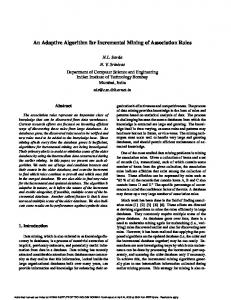
Figure 3: An example constraint graph that illustrates how the propagate degrees of freedom algorithm may be applied to multi-output constraints. The bold-faced edges, constraints, and variable names indicate which portion of the constraint graph is being directed in each panel. The small constraint icons that appear next to constraints 1 and 2 represent the methods that may be used to satisfy these constraints. The propagate degrees of freedom strategy for multi-output constraints is similar to the strategy for single-output constraints. It successively performs the following actions: 1) find a set of variables that are attached to only one constraint and which are output by one of the methods associated with this constraint; 2) make the constraint output these variables by assigning it the method which outputs these variables; and 3) eliminate the constraint and all edges attached to that constraint from the graph. For example, in (c), A and C are attached to only one constraint, and one of the constraint’s three methods (highlighted by bold-faced lines) outputs these variables. Consequently, the propagate degrees of freedom strategy makes constraint 1 output A and C (panel (c)), and then eliminates constraint 1 and its edges from the graph (panel (d)). This procedure is repeated until all constraints have been eliminated from the graph. The resulting directed graph is acyclic, as shown in (e). at least one vertex that is attached to at most one other vertex. Consequently, the modified propagate degrees of freedom algorithm finds an acyclic solution if and only if one exists. It is interesting to note that if the restriction that a method must use every variable in the
QuickPlan
- 10 -
constraint as an input or an output is relaxed (i.e., instead of requiring method.outputs ∪ method.inputs = constraint.variables, we only require method.outputs ∪ method.inputs ⊆ constraint.variables), then it might be possible to make the remaining subgraph acyclic by selecting methods so that some of the edges in the subgraph are removed. However, Maloney has proven that in this case, finding an acyclic graph is NP-complete [33]. Fortunately, constraints in real applications invariably obey this restriction. Thus, in practice, it is possible to exclude constraints that would make constraint satisfaction an NP-complete problem. 5.2.2 Data Structures Table 1 shows the data structures that are used to represent variables, constraints, and methods.
Variable determined_by
the constraint that assigns a value to this variable
constraints
the set of constraints that reference the variable
num_constraints the number of constraints that reference the variable value
the value of the variable (this field is not used by the planning algorithm)
mark
a field that may be used to mark a variable as visited
walkbound
a lower bound on the minimum strength constraint that is upstream of a variable (discussed in Appendix)
Constraint variables
the set of variables that this constraint references
methods
the set of methods that may be used to satisfy this constraint
selected_method the method that currently satisfies the constraint strength
the constraint’s strength in the constraint hierarchy
mark
a field that may be used to mark a constraint as visited
Method outputs the set of variables that this method outputs code
the code that implements this method
Table 1: The data structures that are used to represent variables, constraints, and methods.
QuickPlan
- 11 -
5.2.3 Multi-Output Algorithm The propagate degrees of freedom algorithm for multi-output constraints is formalized in Figure 4. The first line finds all free variables and places them on a stack. The ensuing loop performs the repetitive propagate degrees of freedom search. A free variable is found on line 3 and tested on line 4 to ensure that the constraint to which the variable was attached when the variable was added to the free variable stack has not been eliminated. Lines 5-6 identify the constraint in the graph to which the free variable is attached and a method that outputs a subset of the constraint’s free variables, if one currently exists. In most applications each method has a small number of outputs, so an appropriate method can be found efficiently by examining each method. If each method may have a large number of outputs, a more efficient technique can be employed that involves augmenting each method’s data structure with a count of the number of outputs for that method and a count of the number of outputs that are currently free variables. A free variable can then increment the free variable count of each method that outputs it, and if the free variable count matches the output count, the method can be selected to satisfy the constraint. This technique guarantees O(M) time to locate a method, since a variable can belong to no more than M methods. Lines 9-12 remove the constraint from the graph and determine if the constraint’s removal frees any variables (i.e., decreases the number of constraints that a variable is attached to to one). Global Variables unsatisfied_cns: a set of unsatisfied constraints. free_variable_stack: a stack of free variables. multi_output_planner() (1) free_variable_stack = {v | v is attached to at least one constraint in unsatisfied_cns, v.num_constraints = 1} (2) while (unsatisfied_cns ≠ ∅ and free_variable_stack ≠ ∅) do (3) free_var = pop(free_variable_stack) (4) if free_var.num_constraints = 1 then (5) cn = the constraint cn such that cn ∈ free_var.constraints and cn ∈ unsatisfied_cns (6) if ∃ mt ∈ cn.methods such that ∀ var ∈ mt.outputs, var.num_constraints = 1 then (7) cn.selected_method = mt (8) for each output ∈ mt do output.determined_by = cn (9) for each var ∈ cn.variables do (10) var.num_constraints = var.num_constraints - 1 (11) if var.num_constraints = 1 then push(var, free_variable_stack) (12) unsatisfied_cns = unsatisfied_cns - {cn} Figure 4: multi_output_planner uses the propagate degrees of freedom technique to find acyclic solutions to sets of multi-output constraints.
QuickPlan
- 12 -
5.2.4 Time Complexity In analyzing the time complexity of constraint satisfaction algorithms, it is commonly assumed that the number of variables that belong to a constraint is bounded by a small constant [49, 25, 41, 21]. This assumption is justified in practice and thus will be adopted throughout this paper in the analysis of time complexity. Similarly, in practice the number of methods associated with any constraint is bounded by a small constant, and thus it will be assumed throughout this paper that the number of methods, M, is bounded by a small constant. Under these assumptions, the running time of the multi-output planner is O(N), where N is the number of constraints in the constraint system. This time complexity can be proved by showing that the planner’s time complexity is proportional to the number of edges in the original constraint graph. Since the number of edges is O(N) (each constraint can have no more than a constant number of variables and thus a constant number of edges), the planner’s time complexity will also be O(N). It can be shown that the planner’s time complexity is proportional to the number of edges in the constraint graph as follows. Each variable is processed at most once by the outer loop. The search that finds the unsatisfied constraint which contains the variable may have to examine all of the constraints attached to the variable. The cumulative effect of these searches is to examine each edge in the graph once. Similarly, each constraint is processed at most once by the inner loop. This loop visits each variable attached to the constraint. Again, the cumulative effect of these visits is to examine each edge in the graph once. The only remaining operations of any significance are 1) finding the initial set of free variables, and 2) finding a method to satisfy a constraint. The initial set of free variables can be found by examining each of the variables in the constraint system. This search will examine each of the edges in the constraint graph once, and thus can be performed in O(N) time. A method can be found in O(M) time using the techniques described in the previous section. A method search is performed only when a free variable belongs to an unsatisfied constraint. Since each constraint has a bounded number of variables, the number of method searches must be O(N). Since M is assumed to be bounded by a constant, the time expended in method searches is O(N). Since all of the operations involved in the multi-output planner consume O(N) time, the overall time complexity of the multi-output planner is O(N).
5.3 Constraint Hierarchies The multi-output algorithm presented in the previous section assumes that all constraints must be enforced. This section extends the algorithm to handle constraint hierarchies, so that if all constraints cannot be enforced, then constraints with lesser strengths can be retracted so that greater strength constraints can be enforced. The algorithm described in this section will generate locally-graph-better constraint solutions.
QuickPlan
- 13 -
5.3.1 Overview The propagate degrees of freedom algorithm will operate on a constraint graph as previously described, by recursively attempting to find free variables and to eliminate constraints until all constraints have been satisfied. However, if the algorithm encounters a subgraph in which every variable belongs to two or more constraints then, instead of terminating, it will attempt to retract the weakest strength constraint from the graph, provided that the weakest strength constraint is not a required constraint. The algorithm will then attempt to satisfy the new subgraph. The algorithm will alternate the elimination and retraction steps until it has either eliminated all constraints from the graph or until all the remaining variables are attached to two or more required constraints. Figure 5 illustrates this process on an example graph. If the algorithm is not able to satisfy all the required constraints, then the subgraph consisting of the unsatisfied required constraints is cyclic. If all the constraints are eliminated, then the directed graph constructed by this algorithm is acyclic. The same argument used in Section 5.2.1 to show that a graph is either cyclic or acyclic can be used to prove these two observations. If the constraint solver successfully eliminates all constraints but retracts one or more constraints in doing so, then the generated solution may not be the best possible solution (i.e., it may be possible to find a locally-graph-better solution). For example, the initial solution in Figure 5.g can be improved by reasserting the stay constraint for D and making constraint 3 output C (Figure 5.h). The resulting solution is locally-graph-better than the previous solution because it satisfies the required constraints (constraints 1-3) and satisfies one more constraint at the next (strong) level. To obtain a locally-graph-better solution, the constraint solver can attempt to enforce the retracted constraints in decreasing order of strength. The constraint solver may enforce an additional constraint by executing the modified propagate degrees of freedom algorithm on the union of the set of previously satisfied constraints, and the additional constraint it is trying to enforce. In attempting to enforce the additional constraint, the propagate degrees of freedom algorithm may retract constraints of lesser strength than the constraint it is trying to enforce. However, it may not retract constraints of equal or greater strength, since doing so would lead to a solution that is worse, or at best, no better than, the original solution. Consequently, if the propagate degrees of freedom reaches a point where it would have to retract a constraint of equal or greater strength than the constraint it is trying to enforce, it will terminate and communicate to the constraint solver that it cannot enforce the additional constraint. If the propagate degrees of freedom algorithm succeeds in enforcing the additional constraint, then any constraints that were retracted in order to enforce the constraint are added to the set of constraints that the constraint solver must attempt to enforce. Since the solver attempts to enforce retracted constraints in decreasing strength order, it only has to process each retracted constraint once. If the constraint is successfully enforced, it cannot be retracted by the enforcement of any subsequent constraint. If the constraint is not successfully enforced, only the retraction of an equal or greater strength constraint would allow the constraint to be enforced. However, only retracted constraints of equal or weaker strength will be subsequently enforced. Since the enforcement of these constraints can only result in the retraction of strictly weaker constraints, it will not
QuickPlan
- 14 -
E
strong stay
A
A
2
B
B strong stay
1 3
A
A
1
strong stay
C
(b)
B
B strong stay
1 3
D
A
strong stay
C
(d)
B
B A
1
C
(e)
(f) F
E 2
B
B
C
(g)
3
D
strong stay
A
3
D
3
D
strong stay
F
2
strong stay
D
1
C
1
3
1
(c)
E
strong stay
D
A
(a)
C
strong stay
F
2
C
strong stay
E
F
1 C
strong stay
(h)
Figure 5: An example constraint graph that illustrates how QuickPlan may be applied to multioutput, constraint hierarchies. The bold-faced edges, constraints, and variable names indicate which portion of the constraint graph is being directed in each panel. The small constraint icons that appear next to constraints 1 and 2 represent the methods that may be used to satisfy these constraints. Dashed lines represent unenforced constraints and edges. At each step, QuickPlan either finds a set of free variables that may be output by a constraint, as in panels (b), (d), and (f), or it retracts the weakest remaining constraint, as in panels (c) and (e). Once the graph has been directed, QuickPlan attempts to improve the solution by enforcing additional constraints that were retracted during the development of the initial solution. In this case, it succeeds in enforcing the stay constraint on D (panel (h)).
QuickPlan
- 15 -
be possible to enforce the unsuccessfully enforced constraint. Consequently, it need not be considered again. 5.3.2 Constraint Hierarchy Algorithm The constraint satisfaction algorithm for multi-output, constraint hierarchies is formalized in Figure 6. The algorithm consists of two parts: 1) the modified propagate degrees of freedom algorithm, constraint_hierarchy_planner, that may retract constraints in order to satisfy higher strength constraints, and 2) a high-level solver, constraint_hierarchy_solver, that attempts to find locally-graph-better solutions by successively executing constraint_hierarchy_planner on constraint graphs that contain one additional unenforced constraint. constraint_hierarchy_planner closely resembles the description of the modified propagate degrees of freedom algorithm described in the previous section. The one interesting implementation detail of this algorithm is the handling of the two priority queues, unsatisfied_cns and unenforced_cns_queue. These two queues are ordered by constraint strength. Since the number of different strengths is typically quite small, the priority queues can be efficiently implemented as arrays indexed by strengths. Each array entry points to a list of constraints with the appropriate strength. The array implementation allows the operations that are performed on these priority queues—insertions of constraints and deletion of minimum or maximum strength constraints—to be executed in O(1) time. constraint_hierarchy_solver is responsible for obtaining a locally-graph-better solution. It does do by initially asking constraint_hierarchy_planner to satisfy a constraint graph that consists of all the constraints in the system (lines 1-4). It then attempts to improve the resulting solution (i.e., obtain a locally-graph-better solution) by preparing constraint graphs that consist of the previously satisfied set of constraints and successively weaker retracted constraints (lines 5-14). constraint_hierarchy_solver assumes the responsibility of creating the free_variable_stack, so the initial step in the multi-output planner that computes the free_variable_stack (line 1 in Figure 4) can be deleted. Two aspects of constraint_hierarchy_solver that were not discussed in the previous section are the initialization of each variable’s num_constraints field and the restoration of the previous solution if the enforcement of a retracted constraint fails. A variable’s num_constraints field is set to the number of constraints to which it belongs in the constraint graph that the solver constructs, rather than the total number of constraints to which it belongs. The num_constraints field is not initialized to the total number of constraints because the constraints that are not in the constraint graph are retracted constraints which are considered to be already eliminated. The previous solution can be restored by setting each constraint’s selected_method field to the method that previously satisfied it, and each variable’s determined_by field to the constraint that previously determined it. The information required for restoring the previous solution can be obtained by saving on a stack constraints whose selected methods have been altered, and the constraints’ previous selected methods (a statement to save an altered constraint and its previous selected method can be
QuickPlan
- 16 -
Global Variables unsatisfied_cns: a set of unsatisfied constraints. free_variable_stack: a stack of free variables. unenforced_cns_queue: a priority queue of retracted constraints ordered by decreasing strength. Parameters ceiling_strength: a limit on the maximum strength constraint that may be retracted in order to enforce a constraint. constraint_hierarchy_planner (ceiling_strength : strength) (1) multi_output_planner() (2) while (unsatisfied_cns ≠ ∅ and min_strength(unsatisfied_cns) < ceiling_strength) do (3) cn = delete_min(unsatisfied_cns) (4) unenforced_cns_queue = unenforced_cns_queue ∪ {cn} (5) for each output ∈ cn.selected_method.outputs do output.determined_by = NULL (6) cn.selected_method = NULL (7) for each v ∈ cn.variables do (8) v.num_constraints = v.num_constraints - 1 (9) if v.num_constraints = 1 then push(v, free_variable_stack) (10) multi_output_planner() constraint_hierarchy_solver() (1) unsatisfied_cns = {cn | cn.selected_method = NULL} (2) unenforced_cns_queue = ∅ (3) free_variable_stack = {v | v is attached to at least one constraint in unsatisfied_cns, v.num_constraints = 1} ;; constraints with strength less than required may be revoked (4) constraint_hierarchy_planner(‘‘required’’) (5) if (unsatisfied_cns = ∅) then (6) while unenforced_cns_queue ≠ ∅ do (7) cn = delete_max(unenforced_cns_queue) ;; add cn to the set of constraints that are currently satisfied and ;; make this set the new set of unsatisfied constraints (8) unsatisfied_cns = {cn | cn.selected_method ≠ NULL} ∪ {cn} (9) for each var ∈ {v | v is attached to at least one constraint in unsatisfied_cns} do ;; var.num_constraints is the number of satisfied constraints to which var belongs (10) var.num_constraints = | {cn | cn ∈ var.constraints, cn ∈ unsatisfied_cns} | (11) free_variable_stack = {v | v is attached to at least one constraint in unsatisfied_cns, v.num_constraints = 1} (12) constraint_hierarchy_planner(cn.strength) (13) if unsatisfied_cns ≠ ∅ then ;; the retracted constraint could not be enforced (14) restore the selected_method fields of previously satisfied constraints and the determined_by fields of variables that were output by these constraints to their previous values Figure 6: The constraint satisfaction algorithm for multi-output, constraint hierarchies. The algorithm consists of two parts: 1) a modified propagate degrees of freedom algorithm, constraint_hierarchy_planner, that may retract constraints in order to satisfy higher strength constraints, and 2) a high-level solver, constraint_hierarchy_solver, that attempts to find locally-graph-better solutions by successively executing constraint_hierarchy_planner on constraint graphs that contain one additional unenforced constraint.
QuickPlan
- 17 -
inserted immediately before line 7 in the multi-output algorithm shown in Figure 4). The previous solution can then be restored by popping constraint-method pairs off the stack and assigning the method to the constraint. The variables’ determined_by fields can be restored by first setting the determined_by fields of the failed method’s outputs to null, and then setting the determined_by fields of the restored method’s outputs to the constraint. 5.3.3 Time Complexity The time complexity analysis in this section will show that if the number of variables per constraint is bounded by a constant, then the constraint hierarchy solver requires O(N2) time to construct a locally-graph-better solution. The next section discusses incremental techniques that can generally decrease the solver’s actual running time to O(N). The O(N2) bound on the running time of the constraint solver can be obtained by showing that there may be O(N) iterations of the loop in constraint_hierarchy_solver, and that each iteration requires O(N) time. The loop in constraint_hierarchy_solver attempts to enforce retracted constraints. The loop processes each retracted constraint once. Since there are N constraints, there are potentially O(N) retracted constraints, and thus there may be O(N) iterations of the loop. The significant operations in each loop iteration are 1) the identification of constraints to be satisfied in that iteration, 2) the initialization of the constraints’ mark fields and the initialization of the variables’ num_constraints field, 3) the execution of the propagate degrees of free algorithm, constraint_hierarchy_planner, and 4) the restoration of the previous solution if the retracted constraint cannot be enforced. The identification of constraints and the initialization of their mark fields can be accomplished by examining each constraint once and hence requires O(N) time. The initialization of the num_constraints field examines each edge in the constraint graph once. Since the number of variables per constraint is bounded by a constant, the number of examined edges is O(N). Consequently the initialization of variables can be performed in O(N) time. Similarly, restoring the previous solution if the retracted constraint cannot be enforced can be performed in O(N) time because 1) at most O(N) constraints must have their selected_method field restored, and 2) at most O(N) variables must have their determined_by fields restored because each altered constraint has a bounded number of variables. The only remaining operation is the call to constraint_hierarchy_planner. The primary work of constraint_hierarchy_planner is performed in the propagate degrees of freedom algorithm for multi-output constraints, which requires O(N) time. If the priority queues unsatisfied_cns and unenforced_cns_queue are implemented as arrays, then insertions and delete_min operations can be performed in O(1) time. Since there are N constraints, constraint_hierarchy_planner makes at most N deletions from the unsatisfied_cns queue and at most N insertions to the unenforced_cns_queue. Since the cumulative time expended on these operations is O(N), constraint_hierarchy_planner executes in O(N) time. Since the highest cost operation in any iteration of the constraint solver’s loop requires O(N) time, and since there are O(N) iterations of this loop, the theoretical running time of the constraint
QuickPlan
- 18 -
hierarchy solver is O(N2).
6 Incremental Techniques The planning algorithms presented in the previous section examine the entire constraint graph each time a constraint is added to or removed from the constraint system. However, a change to the constraint system usually perturbs only a local portion of the directed graph, thus making most of this examination unnecessary. This section describes strategies that QuickPlan employs to 1) decrease the number of constraints it must examine, 2) decrease the number of retracted constraints it must attempt to enforce, and 3) terminate early. The algorithms in this section are presented at a high-level to provide a clear explanation of their design. The appendix discusses some of the low-level implementation details that allow these algorithms to be implemented efficiently.
6.1 Overview of the Incremental Techniques 6.1.1 The Upstream Constraint Technique When QuickPlan attempts to enforce a constraint, it only has to examine constraints that are upstream of the variables in the constraint it is attempting to enforce. Constraint cn is upstream of variable v if there is a directed path from cn to v. To understand why only upstream constraints must be examined, let G denote the original undirected constraint graph, let new_cn denote the additional constraint to be enforced, let G’ denote the undirected constraint graph that arises by adding new_cn, and let DG represent the original directed solution graph. Divide the verticies in G’ into two groups. The first group consists of the vertices representing new_cn, its variables, and the variables and constraints that are upstream in DG of new_cn’s variables. The second group contains vertices that are descendents in DG of new_cn’s variables (see Figure 7). Let DGU (for upstream) be the induced subgraph for the vertices in the first group and let DGD (for descendent) be the induced subgraph for the vertices in the second group. The edges in DG that do not appear in either of the subgraphs all point from DGU to DG D.
DGD DGU
Figure 7: A directed constraint graph divided into its upstream (DGU) and downstream (DGD) components by an inserted constraint (the nodes associated with the inserted constraint are shaded black). The boxes denote constraints and the circles denote variables.
If QuickPlan is executed on the entire constraint graph G’, the constraints in DGD will be
QuickPlan
- 19 -
eliminated before any constraints in DGU are eliminated. This observation can be justified by noting that if the edges of DG are reversed, the resulting graph represents the order in which constraints in the original constraint graph G were eliminated. In this reversed graph, all the edges between DGU and DGD are directed toward DGU. Thus, even with the addition of the new constraint new_cn, all the constraints in DGD can be eliminated before the constraints in DGU are considered. A consequence of this observation is that the portion of DG that corresponds to DGD is still valid. Thus, only the edges in the graph corresponding to DGU must be redirected. An algorithm that collects the constraints in DGU is shown in Figure 8. Global Variables unsatisfied_cns: the set of unsatisfied constraints that is being collected. visited_mark: A unique mark that may be assigned to a constraint’s mark field to indicate that the constraint has been visited. collect_upstream_constraints (cn : constraint) (1) cn.mark = visited_mark (2) unsatisfied_cns = unsatisfied_cns ∪ {cn} (3) for each v ∈ cn.variables do (4) e = v.determined_by (5) if e ≠ NULL and e.mark ≠ visited_mark then (6) collect_upstream_constraints(e) Figure 8: collect_upstream_constraints employs a depth-first search to collect all enforced constraints that are upstream of the constraint to be enforced.
6.2 Collecting Unenforced Constraints When a constraint is retracted, either to allow a stronger constraint to be enforced or because it is being removed from the constraint system by a user, it may become possible to enforce other retracted constraints. However, the set of retracted constraints that become potentially enforceable is restricted in a number of ways. First, only constraints of equal or less strength become enforceable. A higher strength constraint cannot become enforceable because, otherwise, the previous solution would not have been locally-graph-better (a locally-graph-better solution could have been constructed by retracting this constraint and enforcing the higher-strength constraint). Since we assume that the previous solution was locally-graph-better, a higher strength constraint must not be enforceable. Second, only retracted constraints attached to either the constraint’s output variables or variables downstream of the output variables become enforceable (Figure 9). These constraints were potentially retracted in order to make the newly revoked constraint enforceable. In contrast, retracted constraints that are upstream of the newly revoked constraint were retracted after the newly revoked constraint was enforced. Consequently, the revocation of this constraint will not allow them to be enforced. Viewed
QuickPlan
- 20 -
from a graph-theoretic perspective, the newly revoked constraint was eliminated before these upstream constraints were retracted. Since revocation has the same effect on the graph as elimination, these upstream constraints will still be uneforceable. An incremental algorithm that takes advantage of these two restrictions is shown in Figure 10.
. . .
... v
v
w
(a)
. . .
⊷⊷⊷⊷⊷⊷⊷⊷⊷⊷⊷⊷⊷⊷⊷⊷⊷⊷⊷⊷ ⊷⊷⊷⊷⊷⊷⊷⊷⊷⊷⊷⊷⊷⊷⊷⊷⊷⊷⊷⊷ ⊷⊷⊷⊷⊷⊷⊷⊷⊷⊷⊷⊷⊷⊷⊷⊷⊷⊷⊷⊷ ⊷⊷⊷⊷⊷⊷⊷⊷⊷⊷⊷⊷⊷⊷⊷⊷⊷⊷⊷⊷ ⊷⊷⊷⊷⊷⊷⊷⊷⊷⊷⊷⊷⊷⊷⊷⊷⊷⊷⊷⊷ ⊷⊷⊷⊷⊷⊷⊷⊷⊷⊷⊷⊷⊷⊷⊷⊷⊷⊷⊷⊷ ⊷⊷⊷⊷⊷⊷⊷⊷⊷⊷⊷⊷⊷⊷⊷⊷⊷⊷⊷⊷ ⊷⊷⊷⊷⊷⊷⊷⊷⊷⊷⊷⊷⊷⊷⊷⊷⊷⊷⊷⊷ ⊷⊷⊷⊷⊷⊷⊷⊷⊷⊷⊷⊷⊷⊷⊷⊷⊷⊷⊷⊷
Legend
constraint to be retracted
(b)
unenforced constraint
unenforced edge
(legend)
Figure 9: When a constraint is retracted, only unenforced constraints downstream of the retracted constraint may become enforceable. Figure (a) illustrates why an unenforced downstream constraint may become enforceable. The dashed-line constraint was retracted in order to allow the blackened constraint to be enforced. Consequently, once the blackened constraint is retracted, the downstream constraint becomes enforceable. In contrast, Figure (b) illustrates why an unenforced upstream constraint remains unenforceable. The dashed-line constraint was retracted after the blackened constraint was enforced (i.e., after the blackened constraint had already been removed from the constraint graph). Since retracting a constraint involves removing it from the constraint graph, and since removing the blackened constraint from the constraint graph will not allow the dashed-line constraint to become enforceable, retracting the blackened constraint will not allow the dashed-line constraint to become enforceable.
Minimizing the Cumulative Number of Visited Variables. Collecting unenforced constraints each time a constraint is retracted could prove somewhat time-consuming because downstream variables that were visited during the retraction of a weaker constraint must be revisited. The reason is that unenforced constraints that are stronger than the weaker constraint must be collected. Fortunately, it is possible to defer the collection of unenforced constraints until a constraint has been enforced. In addition, all of the unenforced constraints that must be examined are attached either to redetermined variables or to variables downstream of the redetermined variables. Consequently, one comprehensive search for unenforced constraints may be performed by searching downstream of the redetermined variables. A redetermined variable is a variable that is either determined by a different constraint or is undetermined. An undetermined variable is not determined by a constraint (such variables are also called input variables because they are not output by any constraint). The following theorem demonstrates that a search that is initiated at redetermined variables will collect all potentially enforceable constraints that are downstream of the retracted constraints. Theorem 1: Let G represent the directed graph obtained by enforcing a new constraint. All constraints that become enforceable as a result of enforcing this new constraint are attached to either the redetermined variables or variables downstream of the redetermined variables.
QuickPlan
- 21 -
Global Variables unenforced_cns_queue: a priority queue of retracted constraints ordered by decreasing strength. search_mark: a unique mark that may be assigned to a constraint’s or a variable’s mark field to indicate that the constraint or variable has been visited. collect_unenforced_constraints(v : variable, ceiling_strength : strength) (1) v.mark = search_mark (2) unenforced_cns_queue = unenforced_cns_queue ∪ {cn | cn ∈ v.constraints, cn.selected_method = NULL, cn.strength ≤ ceiling_strength} (3) for each cn ∈ v.constraints do (4) if (cn.selected_method ≠ NULL and cn.mark ≠ search_mark) then (5) cn.mark = search_mark (6) for each w ∈ cn.selected_method.outputs do (7) if w.mark ≠ search_mark then (8) collect_unenforced_constraints(w, ceiling_strength) Figure 10: collect_unenforced_constraints collects all unenforced constraints whose strength is less than or equal to ceiling_strength and that are either attached to v or are downstream of v. The unenforced constraints downstream of a retracted constraint can be found by calling collect_unenforced_constraints on each of the retracted constraint’s outputs.
Proof: The proof must show that all variables which were downstream of the retracted constraints are either redetermined variables or downstream of redetermined variables. The proof can be performed by induction on the length of the shortest path from any retracted constraint to a downstream variable. The length of a path is defined as the number of constraints on the path from a retracted constraint to a downstream variable. Base Case (length = 0): The variables output by a retracted constraint are reached by a zero-length path from the retracted constraint. These variables will either be output by a new constraint or will be undetermined. In either case, they are redetermined. Inductive Case (length = n): Assume that all downstream variables that could originally be reached by a path of (n-1) constraints from one of the retracted constraints’ outputs conform to the inductive hypothesis. Let v be a variable that was reachable via a path of n constraints (i.e., v was an output of the nth constraint). There are three possible cases: 1. The nth constraint uses the same method. In this case v is still an output of the nth constraint. Further, one of the constraint’s input variables was formerly reachable by a path of (n-1) constraints. The input variable that matches this description satisfies the induction hypothesis. Consequently v is downstream of a redetermined variable, and thus also satisfies the inductive hypothesis. 2. The nth constraint uses a different method, but v is still output by the nth constraint. In this case at least one of the constraint’s prior outputs has become an input. If none of the prior outputs has become an input, then the planning algorithm assigned the constraint a method that outputs a superset of the constraint’s old outputs. However, if the planner has a choice between choosing the previous method or a method that
QuickPlan
- 22 -
outputs a superset of the constraint’s previous outputs, it will choose the previous method, a contradiction. Consequently, if a new method has been assigned to the constraint, at least one of the former output variables is an input variable. This input variable has clearly been redetermined. Consequently v is downstream of at least one redetermined variables, thus satisfying the inductive hypothesis. 3. The nth constraint uses a different method and v is now an input to the nth constraint. In this case v must have been redetermined, because it was formerly an output of the nth constraint. Thus v satisfies the inductive hypothesis. Since all three cases satisfy the inductive hypothesis, the inductive hypothesis has been proved. An incremental algorithm can take advantage of this theorem by maintaining a list of redetermined variables during the planner’s enforcement phase, and then collecting unenforced constraints downstream of these variables once the enforcement phase is complete. This technique is integrated into the incremental version of QuickPlan presented in Section 6.4. The appendix proves a stronger version of this theorem which shows that all redetermined variables are downstream of either undetermined variables or the outputs of the enforced constraint. It then shows how the undetermined variables can be efficiently determined with a minimal consumption of storage.
6.3 Early Termination Once the constraint to be enforced is eliminated from the constraint graph (i.e., QuickPlan assigns a method to satisfy it), the planner may terminate because the remaining constraints in DGU can be enforced by their currently assigned method. The correctness of this observation can be shown by noting that once the targeted constraint has been enforced, the remaining constraint graph is a subgraph of DGU. Since the targeted constraint has been removed from this subgraph, the subgraph has the same set of free variables that existed before the targeted constraint was added to the constraint graph. Consequently, the subgraph can be eliminated using the same set of method assignments that was originally used to eliminate it. To terminate early, the termination conditions in multi_output_planner and constraint_hierarchy_planner must be changed so that rather than checking whether the set of unsatisfied constraints is empty, they check whether the constraint to be enforced has been satisfied (i.e., assigned a method).
6.4 Incremental Algorithm This section incorporates the incremental techniques described in the previous section into the constraint hierarchy planner described in Section 5. It then defines an add_constraint procedure and a remove_constraint procedure that provide entry points to QuickPlan for adding constraints to and removing constraints from the constraint system. Figures 11-13 present incremental versions of multi_output_planner, constraint_hierarchy_planner and constraint_hierarchy_solver that incorporate the techniques described in the previous section. The changes that have been made to the non-
QuickPlan
- 23 -
incremental versions of these algorithms are described by comments and highlighted in either italics or boldface. Old Global Variables unsatisfied_cns, free_variable_stack New Global Variables cn_to_enforce: The constraint the planner is attempting to enforce. redetermined_variables: The set of variables that are determined by either a different constraint or are newly undetermined. multi_output_planner() (2) while (cn_to_enforce.selected_method = NULL and free_variable_stack ≠ ∅) do (3) free_var = pop(free_variable_stack) (4) if free_var.num_constraints = 1 then (5) cn = the constraint cn such that cn ∈ free_var.constraints and cn ∈ unsatisfied_cns (6) if ∃ mt ∈ cn.methods such that ∀ var ∈ mt.outputs, var.num_constraints = 1 then ;; the determined_by fields of the old outputs must be set to NULL ;; since they are no longer determined by any constraint (6-1) for each var ∈ cn.selected_method.outputs do (6-2) var.determined_by = NULL ;; add the constraint’s old and new outputs to the set of redetermined variables (6-3) redetermined_variables = redetermined_variables ∪ cn.selected_method.outputs ∪ mt.outputs (7) cn.selected_method = mt (8) for each output ∈ mt do output.determined_by = cn (9) for each var ∈ cn.variables do (10) var.num_constraints = var.num_constraints - 1 (11) if var.num_constraints = 1 then push(var, free_variable_stack) (12) unsatisfied_cns = unsatisfied_cns - {cn} Figure 11: The version of multi_output_planner in Figure 4 has been modified so that 1) it omits the initial computation of the free variable stack (constraint_hierarchy_solver now performs this computation), 2) it terminates once it assigns a method to the constraint it is attempting to enforce, and 3) it records redetermined variables. Italicized line numbers denote statements that have replaced a previous statement. Boldfaced line numbers denote statements that have been added. In addition, the line numbers used in the presentation of the original version of the algorithm are repeated here to further emphasize the similarities and differences between the two algorithms. Line numbers with dashed numerals (e.g., (6-1), (6-2)) denote a block of statements that has been inserted between two statements in the previous version of the algorithm.
Note that since the constraint planner updates an existing solution, the first five lines of constraint_hierarchy_solver that computed a solution from scratch have been deleted. These lines must be replaced with procedures that either add a constraint to the constraint system (add_constraint) or remove a constraint from the constraint system (remove_constraint). Since the incremental planner operates on a set of unenforced constraints, add_constraint and
QuickPlan
- 24 -
Old Global Variables unsatisfied_cns, free_variable_stack New Global Variables cn_to_enforce: The constraint the planner is attempting to enforce. strongest_retracted_strength: The strength of the strongest constraint retracted in order to enforce cn_to_enforce. The constraint solver only has to attempt to enforce retracted constraints whose strength is less than or equal to strongest_retracted_strength. redetermined_variables: The set of variables that are determined by either a different constraint or are newly undetermined. constraint_hierarchy_planner (ceiling_strength : strength) (1) multi_output_planner() ;; The planner can terminate once it assigns a method to the constraint it is attempting to ;; enforce, rather than waiting until all unsatisfied constraints have been eliminated (2) while (cn_to_enforce.selected_method = NULL and min_strength(unsatisfied_cns) < ceiling_strength) do (3) cn = delete_min(unsatisfied_cns) ;; Retracted constraints are no longer collected here, but rather after the constraint has ;; been enforced. For now, just record the strength of the strongest retracted constraint. (4) strongest_retracted_strength = max(strongest_retracted_constraint, cn.strength) (5) for each output ∈ cn.selected_method.outputs do output.determined_by = NULL (5-1) redetermined_variables = redetermined_variables ∪ cn.selected_method.outputs (6) cn.selected_method = NULL (7) for each v ∈ cn.variables do (8) v.num_constraints = v.num_constraints - 1 (9) if v.num_constraints = 1 then push(v, free_variable_stack) (10) multi_output_planner() Figure 12: The version of constraint_hierarchy_planner presented in Figure 6 has been updated so that it 1) terminates once it succeeds in assigning a method to the constraint it is attempting to enforce, 2) records the strength of the strongest constraint retracted in order to enforce the constraint, and 3) records redetermined variables. Statements that have been changed are italicized and statements that have been added are boldfaced. In addition, the line numbers used in the presentation of the original version of the algorithm are repeated here to further emphasize the similarities and differences between the two algorithms. denote a block of statements that has been inserted between two statements in the previous version of the algorithm. Line numbers with dashed numerals (e.g., (5-1)) denote statements that have been inserted between two statements in the previous version of the algorithm.
remove_constraint can be easily constructed if they define the constraints they add or remove in terms of unenforced constraints. add_constraint treats a new constraint as an unenforced constraint. Consequently, add_constraint initializes the unenforced constraint queue to the new constraint. remove_constraint treats the constraint to be removed as a retracted constraint. Thus remove_constraint initializes the unenforced constraint queue to the set of unenforced constraints
QuickPlan
- 25 -
Old Global Variables unsatisfied_cns, unenforced_cns_queue, free_variable_stack New Global Variables cn_to_enforce: The constraint the planner is attempting to enforce. strongest_retracted_strength: The strength of the strongest constraint retracted in order to enforce cn_to_enforce. visited_mark: A unique mark that may be assigned to a constraint’s mark field as upstream constraints are collected to indicate that the constraint has been visited. search_mark: a unique mark that may be assigned to a constraint’s or a variable’s mark field as unenforced constraints are collected to indicate that the constraint or variable has been visited. redetermined_variables: The set of variables that are determined by either a different constraint or are newly undetermined. constraint_hierarchy_solver() (6) while unenforced_cns_queue ≠ ∅ do (7) cn_to_enforce = delete_max(unenforced_cns_queue) ;; initialize the variables that are required to implement the incremental techniques (7-1) visited_mark = GenerateUniqueMark() (7-2) search_mark = GenerateUniqueMark() ;; *weakest_constraint_strength* is a constant denoting the weakest possible ;; constraint strength (7-3) strongest_retracted_strength = *weakest_constraint_strength* (7-4) unsatisfied_cns = ∅ (7-5) redetermined_variables = ∅ ;; collect only enforced constraints that are upstream of the constraint to enforce (8) collect_upstream_constraints(cn_to_enforce) (9) for each var ∈ {v | v is attached to at least one constraint in unsatisfied_cns} do ;; var.num_constraints is the number of satisfied constraints to which var belongs (10) var.num_constraints = | {cn | cn ∈ var.constraints, cn ∈ unsatisfied_cns} | (11) free_variable_stack = {v | v is attached to at least one constraint in unsatisfied_cns, v.num_constraints = 1} (12) constraint_hierarchy_planner(cn_to_enforce.strength) (13) if cn_to_enforce.selected_method = NULL then (14) restore the selected_method fields of previously satisfied constraints and the determined_by fields of variables that were output by these constraints to their previous values (15) else ;; the constraint has been successfully enforced—collect unenforced constraints ;; that are downstream of the redetermined variables and whose strength is ;; equal to or less than the strength of the strongest retracted constraint (16) for each v ∈ redetermined_variables do (17) collect_unenforced_constraints(v, strongest_retracted_strength) Figure 13: The version of constraint_hierarchy_solver presented in Figure 6 has been updated so that it 1) adds only constraints upstream of the constraint to enforce to the unsatisfied_cns queue, and 2) collects unenforced constraints that are downstream of redetermined variables and whose strength is equal to or less than the strength of the strongest retracted constraint. Italicized line numbers denote statements that have replaced a previous statement. Boldfaced line numbers denote statements that have been added. In addition, the line numbers used in the presentation of the original version of the algorithm are repeated here to further emphasize the similarities and differences between the two algorithms. Line numbers with dashed numerals (e.g., (7-1), (7-2)) denote a block of statements that has been inserted between two statements in the previous version of the algorithm.
QuickPlan
- 26 -
that are downstream of the removed constraint, and that are of equal or lesser strength. add_constraint and remove_constraint procedures are shown in Figures 14 and 15.
The
Global Variables unenforced_cns_queue: a priority queue of unenforced constraints that the constraint solver should attempt to enforce. The queue is ordered by decreasing strength. add_constraint (cn_to_add : constraint) (1) for each v ∈ cn_to_add.variables do (2) v.constraints = v.constraints ∪ {cn_to_add} (3) if ∃ mt ∈ cn_to_add.methods such that for each v ∈ mt.outputs, | v.constraints = 1 | then (4) cn_to_add.selected_method = mt (5) for each v in mt.outputs do v.determined_by = cn_to_add (6) else (7) unenforced_cns_queue = {cn_to_add} (8) constraint_hierarchy_solver() Figure 14: add_constraint attempts to satisfy the new constraint by finding a method that outputs the constraint’s free variables, if any exist. Otherwise it treats the constraint as an unenforced constraint and attempts to enforce it using the constraint planner. If the constraint has enough free variables to allow the constraint to be satisfied, the constraint planner does not have to be called since no constraints will be retracted, and thus the unenforced_cns_queue will be empty.
Global Variables unenforced_cns_queue: a priority queue of unenforced constraints that the constraint solver should attempt to enforce. The queue is ordered by decreasing strength. remove_constraint (cn_to_remove : constraint) (1) unenforced_cns_queue = ∅ (2) for each v ∈ cn_to_remove.variables do (3) v.constraints = v.constraints - {cn_to_remove} (4) if v.determined_by = cn_to_remove then (5) collect_unenforced_constraints(v, cn_to_remove.strength) (6) constraint_hierarchy_solver() Figure 15: remove_constraint treats the removed constraint as a retracted constraint. Consequently, it collects all unenforced constraints of equal or lower strength downstream of the removed constraint’s output variables.
QuickPlan
- 27 -
6.5 Time Complexity The incremental techniques described in this section do not change the worst case running time of the planning algorithm. It is still O(N2). This worst case time complexity can be obtained by observing that there may be O(N) upstream constraints of the constraint to be enforced, which will take O(N) time to collect and eliminate. Collecting unenforced constraints may take O(N) time since the portion of the graph downstream of the redetermined variables may contain O(N) constraints. Thus enforcing a constraint and then collecting any unenforced constraints downstream of the retracted constraints requires O(N) time. In the worst case, the cumulative number of collected unenforced constraints is O(N) (an unenforced constraint is not collected or processed more than once). Consequently, in the worst case, the planner must attempt to enforce O(N) constraints, each of which may require O(N) time, for a worst case time of O(N2). In practice however, the observed running time of the incremental algorithm is actually linear, and in many cases, sublinear, in the number of constraints in the constraint system. There are a number of factors that contribute to this better actual-case performance: 1. The constraint graph is often divided into several completely disjoint subgraphs. Thus, even if the incremental algorithm exhibits its worst case behavior, it will only examine a fraction of the constraints in the constraint system. 2. The number of constraints upstream of a constraint to be enforced is typically only a small fraction of the constraints in the subgraph that is being examined. In many cases this number is O(1), because an input constraint (a constraint that assigns a value to a variable) is overriding a previously enforced stay constraint. Since the stay constraint has no constraints upstream of it, the planner examines only the stay constraint, retracts it, and enforces the input constraint. 3. The collection of unenforced constraints can often be avoided because it can be determined a priori that no unenforced constraints have become enforceable. Two cases in particular often arise. First, no constraint may have to be retracted in order to enforce a constraint. Since no constraints are retracted, no previously unenforceable constraints can become enforceable. Second, an input constraint may be used to override a previously enforced stay constraint. In this case, a stronger constraint is placed on precisely the same set of variables as the previously enforced constraint. Consequently, the same set of constraints that were retracted to enforce the stay constraint must be retracted to enforce the input constraint. Thus no previously unenforceable constraint can become enforceable. 4. Even when the collection of unenforced constraints cannot be avoided, the number of unenforced constraints collected is often bounded by a small constant. Two factors contribute to this small constant. First, many interactive systems often have very few unenforced constraints. Second, the unenforced constraints are almost always stay constraints, and very few of these constraints are typically found downstream of a newly enforced constraint. To illustrate how these factors may interact to permit sublinear performance, consider one of the most frequent uses for multi-way constraints—maintaining consistency between an application’s data and graphical views of this data. These systems typically place stay constraints on the application’s data and no stay constraints on the graphical views of the data (Figure 17 shows the star-shaped constraint graphs that arise from these systems). The most common case is that all constraints, including the stay constraints are enforced. New values are assigned to application variables using input constraints. These
QuickPlan
- 28 -
constraints override an enforced stay constraint, and thus take O(1) time to enforce. It can be determined a priori that no unenforced constraints become enforceable, and thus the addition of an input constraint takes O(1) time. New values may also be assigned to the graphical variables via input constraints. In this case, only two constraints are upstream of the new constraint (see Figure 17) and only the stay constraint on the appropriate application variable must be retracted. Again, the enforcement of the input constraint and the retraction of the stay constraint can be accomplished in O(1) time. The above observations are incorporated in the more detailed algorithms presented in the appendix.
7 Empirical Performance The previous three sections have described the QuickPlan algorithm and have shown that its theoretical time complexity is better than the time complexity of the fastest known algorithm, SkyBlue. This section presents timing results from benchmarks and real applications that indicate that QuickPlan is competitive with or faster than SkyBlue on problems that both algorithms can solve efficiently. The timing results also indicate that QuickPlan delivers excellent performance on problems that SkyBlue either cannot solve (i.e., cannot construct an acyclic solution for) or cannot solve efficiently. The QuickPlan algorithm has been implemented in Multi-Garnet, a research platform developed at the University of Washington as a basis for research on multi-way constraints [42]. Multi-Garnet is an extension to Carnegie Mellon’s widely-used Garnet user interface toolkit [35]. SkyBlue is the constraint solver used in the current release of Multi-Garnet. For the experiments described in this paper, a second version of Multi-Garnet was used that employed QuickPlan rather than SkyBlue. Both the SkyBlue and QuickPlan versions of Multi-Garnet are implemented in CommonLisp. The tests were conducted on an HP750 workstation using X Windows. All tests were repeated 20 times.
7.1 Benchmarks The algorithms were run against two sets of benchmarks. The first set of benchmarks is described in [39] and involve single-output, acyclic constraint hierarchies. SkyBlue runs efficiently on these types of constraint hierarchies. The second set of benchmarks are modified versions of the first set of benchmarks and involve multi-output, cyclic constraint hierarchies. SkyBlue is not guaranteed to run efficiently on these types of hierarchies nor is it guaranteed to produce acyclic solutions. The performance reported for QuickPlan and SkyBlue includes the amount of time each algorithm requires to redirect the constraint graph in order to enforce an added constraint (i.e., the amount of time required by the planning phase). The amount of time required to extract a plan (i.e., collect the set of constraints that must be executed) and execute the plan (i.e., the amount of time required to execute the constraints) are not shown because these operations can be performed by a one-way constraint solver. Consequently, the times required to extract and execute the plan do not reflect differences between the two algorithms (if the two algorithms produced different directed graphs, these times might be relevant;
QuickPlan
- 29 -
however, on the benchmarks that both algorithms successfully complete, the two algorithms construct identical graphs). 7.1.1 Single-Output, Acyclic Constraint Hierarchies The benchmarks that create single-output, non-cyclic constraint hierarchies are summarized in Table 2 and illustrated in Figures 16-18. The results can be analyzed as follows: chain benchmark. QuickPlan and SkyBlue both require O(N) time because they must reverse all the edges in the constraint graph. QuickPlan runs more quickly because it maintains less overhead information than SkyBlue. For each variable, SkyBlue computes a minimum bound on the weakest strength constraint that is upstream of the variable—this bound is called a walkbound3. All variables that are downstream of either a newly enforced constraint or a newly undetermined variable must have their walkbounds updated. In the chain benchmark, there are O(N) variables downstream of the input constraint, and thus O(N) variables must have their walkbounds updated. star benchmark. QuickPlan requires O(1) time because an input constraint is being used to override an enforced stay constraint. SkyBlue requires O(N) time because it must update the walkbounds of all variables downstream of the new input constraint. tree benchmark. QuickPlan requires O(N) time because it examines constraints in all branches of the tree. SkyBlue requires O(log N) time, because it examines constraints in only one branch of the tree. In this case, searching only one branch works because the graph is acyclic. However, in cases where the constraint hierarchy is cyclic, as in the set of benchmarks discussed in the next section, this strategy can produce a cyclic solution when an acyclic solution exists. Table 2: Time required by QuickPlan and SkyBlue on benchmarks involving single-output, acyclic constraint hierarchies. Benchmark
Description
QuickPlan SkyBlue
Chain
Chain of equality constraints
O(N)
O(N)
Star
Star-shaped network in which each constraint references a common variable
O(1)
O(N)
Tree
Tree-shaped network in which each node computes its sum from the values of its children O(N)
O(log N)
3The appendix describes how QuickPlan may also compute walkbounds. However, QuickPlan only computes walkbounds in rare instances when the number of unenforced constraints collected exceeds a threshold. The only benchmark on which QuickPlan computes walkbounds is the multi-tree benchmark described in the next section.
QuickPlan
- 30 -
Strong Input
v1
v2
⊷⊷⊷⊷⊷⊷⊷⊷⊷⊷⊷⊷⊷⊷⊷⊷⊷⊷⊷⊷⊷ ⊷⊷⊷⊷⊷⊷⊷⊷⊷⊷⊷⊷⊷⊷⊷⊷⊷⊷⊷⊷⊷ ⊷⊷⊷⊷⊷⊷⊷⊷⊷⊷⊷⊷⊷⊷⊷⊷⊷⊷⊷⊷⊷ ⊷⊷⊷⊷⊷⊷⊷⊷⊷⊷⊷⊷⊷⊷⊷⊷⊷⊷⊷⊷⊷ ⊷⊷⊷⊷⊷⊷⊷⊷⊷⊷⊷⊷⊷⊷⊷⊷⊷⊷⊷⊷⊷ ⊷⊷⊷⊷⊷⊷⊷⊷⊷⊷⊷⊷⊷⊷⊷⊷⊷⊷⊷⊷⊷ ⊷⊷⊷⊷⊷⊷⊷⊷⊷⊷⊷⊷⊷⊷⊷⊷⊷⊷⊷⊷⊷ ⊷⊷⊷⊷⊷⊷⊷⊷⊷⊷⊷⊷⊷⊷⊷⊷⊷⊷⊷⊷⊷ ⊷⊷⊷⊷⊷⊷⊷⊷⊷⊷⊷⊷⊷⊷⊷⊷⊷⊷⊷⊷⊷
v3
...
vn - 1
vn
Weak Stay
Legend
v1
v2
v3
vn - 1
...
vn
Weak Stay
newly added constraint
(a)
newly unenforced constraint
redirected edge
newly unenforced edge
(b) 3000
milliseconds
2500
2000 SkyBlue QuickPlan
1500
1000
500
0 0
5000
10000
15000
20000
number of constraints
(c) Figure 16: The chain benchmark assigns a new value to the variable at the head of a chain of equality constraints, v1 = v2 = v3 = ... = vn. (a) A weak stay constraint on vn initially causes values to be propagated from vn to v1. (b) The benchmark creates an input constraint that assigns a new value to v1. The input constraint is enforced by retracting the stay constraint on vn and reversing all the edges in the constraint graph. (c) The average time required by QuickPlan and SkyBlue to enforce the input constraint.
7.1.2 Multi-Output, Cyclic Constraint Hierarchies The benchmarks that create multi-output, non-cyclic constraint hierarchies are summarized in Table 3 and illustrated in Figures 19-21. In each of the benchmarks, a constraint has four variables and six methods. Each method outputs two of the constraint’s four variables by assigning the two input variables to the two output variables (e.g., x1, y1 = x2, y2). The results can be analyzed as follows: multi-chain benchmark. QuickPlan executes in O(N) time because it must redirect half the edges in the constraint graph. It requires approximately twice the time it required on the single-output benchmark. This time requirement is reasonable since there are twice as many edges in the graph and QuickPlan must examine each of them. SkyBlue executes in O(N2) time on this benchmark because the strategy it employs causes it to perform backtracking. This strategy attempts to ‘‘grow’’ a plan by successively adding constraints with new selected methods. If SkyBlue finds that adding a constraint would cause a conflict with another constraint in the plan (i.e., the constraints would output to a common variable), SkyBlue backtracks by popping constraints off the plan and attempting to grow the plan using
QuickPlan
- 31 -
scaled_value1
Weak Stay
data1
scaled_value1
Weak Stay
Weak Stay
data1 Strong Input
scaled_valuen
Weak Stay
scaled_valuen
scaled_value2 scale_factor ...
datan
data2
Weak Stay
Weak Stay
...
scaled_valuen - 1
datan - 1
scaled_valuen - 1
scaled_value2
scale_factor
datan
⊷⊷⊷⊷⊷⊷⊷⊷⊷⊷⊷⊷⊷⊷⊷⊷⊷⊷⊷⊷⊷ ⊷⊷⊷⊷⊷⊷⊷⊷⊷⊷⊷⊷⊷⊷⊷⊷⊷⊷⊷⊷⊷ ⊷⊷⊷⊷⊷⊷⊷⊷⊷⊷⊷⊷⊷⊷⊷⊷⊷⊷⊷⊷⊷ ⊷⊷⊷⊷⊷⊷⊷⊷⊷⊷⊷⊷⊷⊷⊷⊷⊷⊷⊷⊷⊷ ⊷⊷⊷⊷⊷⊷⊷⊷⊷⊷⊷⊷⊷⊷⊷⊷⊷⊷⊷⊷⊷ ⊷⊷⊷⊷⊷⊷⊷⊷⊷⊷⊷⊷⊷⊷⊷⊷⊷⊷⊷⊷⊷ ⊷⊷⊷⊷⊷⊷⊷⊷⊷⊷⊷⊷⊷⊷⊷⊷⊷⊷⊷⊷⊷ ⊷⊷⊷⊷⊷⊷⊷⊷⊷⊷⊷⊷⊷⊷⊷⊷⊷⊷⊷⊷⊷ ⊷⊷⊷⊷⊷⊷⊷⊷⊷⊷⊷⊷⊷⊷⊷⊷⊷⊷⊷⊷⊷
Weak Stay
datan - 1
Weak Stay
data2
Weak Stay
Legend
Weak Stay
newly added constraint
newly unenforced constraint
(a)
redirected edge
newly unenforced edge
(b)
milliseconds
1500
1000 SkyBlue QuickPlan 500
0.260 0
5000
10000
15000
20000
number of constraints
(c) Figure 17: The star benchmark assigns a new value to a scale factor that is referenced by every constraint in a star-shaped network. The network is constructed by creating constraints that scale a set of data points (scaled_valuei = scale_factor × datai). (a) A weak stay constraint on the scaling factor and the data points initially cause the constraints to be solved for the scaled value. (b) The benchmark creates an input constraint that assigns a new value to scale_factor, thus overriding the stay constraint. (c) The average time required by QuickPlan and SkyBlue to enforce the input constraint.
different constraints. This technique is described in more detail in the related work section (Section 8). In addition to backtracking, SkyBlue also constructs a cyclic solution that does not correctly implement the benchmark. multi-star benchmark. QuickPlan executes in O(1) time because it involves overriding a stay constraint with an input constraint. SkyBlue executes in O(N) time because it does not perform backtracking on this benchmark. In this case, the sharing of two common variables by all constraints places a linear bound on the number of possible ways to direct the constraint graph.
QuickPlan
- 32 -
⊷⊷⊷⊷⊷⊷⊷⊷⊷⊷⊷⊷⊷⊷⊷⊷⊷⊷⊷⊷⊷ ⊷⊷⊷⊷⊷⊷⊷⊷⊷⊷⊷⊷⊷⊷⊷⊷⊷⊷⊷⊷⊷ ⊷⊷⊷⊷⊷⊷⊷⊷⊷⊷⊷⊷⊷⊷⊷⊷⊷⊷⊷⊷⊷ ⊷⊷⊷⊷⊷⊷⊷⊷⊷⊷⊷⊷⊷⊷⊷⊷⊷⊷⊷⊷⊷ ⊷⊷⊷⊷⊷⊷⊷⊷⊷⊷⊷⊷⊷⊷⊷⊷⊷⊷⊷⊷⊷ ⊷⊷⊷⊷⊷⊷⊷⊷⊷⊷⊷⊷⊷⊷⊷⊷⊷⊷⊷⊷⊷ ⊷⊷⊷⊷⊷⊷⊷⊷⊷⊷⊷⊷⊷⊷⊷⊷⊷⊷⊷⊷⊷ ⊷⊷⊷⊷⊷⊷⊷⊷⊷⊷⊷⊷⊷⊷⊷⊷⊷⊷⊷⊷⊷ ⊷⊷⊷⊷⊷⊷⊷⊷⊷⊷⊷⊷⊷⊷⊷⊷⊷⊷⊷⊷⊷
Legend
Strong Input
newly added constraint newly unenforced constraint
Node11
Node11
redirected edge newly unenforced edge
Node21
Node31
Leaf1
Leaf2
Weak Weak Stay Stay
Node22
Node32
Leaf3
Leaf4
Weak Weak Stay Stay
Node33
Leaf5
Node34
Leaf6
Weak Weak Stay Stay
Node21
Leaf7
Node31
Leaf8
Leaf1
Weak Weak Stay Stay
Leaf2
Weak Weak Stay Stay
Node22
Node32
Leaf3
Node33
Leaf4
Leaf5
Weak Weak Stay Stay
(a)
Leaf6
Weak Weak Stay Stay
Node34
Leaf7
Leaf8
Weak Weak Stay Stay
(b) 402
milliseconds
100
SkyBlue QuickPlan 10 7
2.6 1.5 256
512
1024
2048
4096
8192
16384
number of constraints
(c) Figure 18: The tree benchmark assigns a new value to the root of a binary tree in which every node computes its sum from the values of its two children. (a) Weak stay constraints on the leaves of the tree initially cause values to flow from the leaves of the tree to the root. (b) The benchmark creates an input constraint that assigns a new value to the root node. The input constraint is enforced by retracting the stay constraint on one of the leaves and reversing the edges in the constraint graph on the path between the root and this leaf. (c) The average time required by QuickPlan and SkyBlue to enforce the input constraint.
multi-tree benchmark. QuickPlan executes in O(N log N) time because it must attempt to enforce all the weak stay constraints that have been retracted. This time is obtained by observing that for each retracted stay constraint, QuickPlan examines each constraint on the path between the stay constraint and the root of the tree. Because there are O(log N) such constraints, and because there are O(N) stay constraints, QuickPlan executes in O(N log N) time. SkyBlue performs backtracking on this problem and requires O(N2 log N) time. It also constructs a cyclic solution that does not correctly implement the
QuickPlan
- 33 -
benchmark. Table 3: Time required by QuickPlan and SkyBlue on benchmarks involving multi-output, cyclic constraint hierarchies. The ‘‘cycle’’ entry for SkyBlue on the multi-chain and multi-tree benchmarks indicate that SkyBlue constructed a cyclic rather than an acyclic solution, and thus did not correctly implement the benchmark. Benchmark
Description
Multi-Chain Chain of constraints
QuickPlan
SkyBlue
O(N)
Cycle O(N2)
O(1)
O(N)
Multi-Star
Star-shaped network in which each constraint references two common variables
Multi-Tree
Cycle Tree-shaped network in which each node is involved in a constraint that references its children and its sibling O(N log N) O(N 2 log N)
7.2 Applications The following three subsections describe the performance of several real applications that were implemented using the QuickPlan version of Multi-Garnet. The applications include a user interface for visualizing statistical data (provided with the Multi-Garnet release), a user interface for visualizing binary trees, and a user interface for manipulating formatted lists of objects. In each of the applications, QuickPlan is fast enough to support interactive manipulation of the graphical objects. As in the previous section, the performance reported for QuickPlan includes the amount of time it requires to redirect the constraint graph in order to implement a user interface action. To place these times in perspective, the amount of time required for all other operations (e.g., extracting a plan, executing a plan, redrawing graphical objects, and identifying the objects to be manipulated) is also reported. Finally, planning times are also reported for SkyBlue. The applications and performance results for representive operations are summarized in Table 4 and illustrated in Figures 22-24. The results can be analyzed as follows: Scatterplot Interface. The constraints in the scatterplot interface conform to an acyclic, multioutput constraint hierarchy. QuickPlan requires O(1) time to scale the data points, since the constraints form a star-like network. SkyBlue require O(N) time to scale the data points, since the plan it creates places all the scaling constraints downstream of the scaled point. Thus O(N) walkbounds must be updated. Both algorithms require O(1) time to move the x-axis, since only the constraints that affect the text labels are examined. SkyBlue requires O(1) time in this case because only a constant number of constraints must have their walkbounds updated. QuickPlan is somewhat faster on this operations because it does not have to compute walkbounds. Binary Tree Interface. The constraints in the binary tree interface conform to a single-output,
QuickPlan
v1
- 34 -
v2
v3
vn - 1
vn
Weak Stay
wn - 1
wn
Weak Stay
... w1
w2
w3
Strong Input
v1
v2
v3
vn - 1
vn
Weak Stay
wn - 1
wn
Weak Stay
... w1
w2
⊷⊷⊷⊷⊷⊷⊷⊷⊷⊷⊷⊷⊷⊷⊷⊷⊷⊷⊷⊷⊷ ⊷⊷⊷⊷⊷⊷⊷⊷⊷⊷⊷⊷⊷⊷⊷⊷⊷⊷⊷⊷⊷ ⊷⊷⊷⊷⊷⊷⊷⊷⊷⊷⊷⊷⊷⊷⊷⊷⊷⊷⊷⊷⊷ ⊷⊷⊷⊷⊷⊷⊷⊷⊷⊷⊷⊷⊷⊷⊷⊷⊷⊷⊷⊷⊷ ⊷⊷⊷⊷⊷⊷⊷⊷⊷⊷⊷⊷⊷⊷⊷⊷⊷⊷⊷⊷⊷ ⊷⊷⊷⊷⊷⊷⊷⊷⊷⊷⊷⊷⊷⊷⊷⊷⊷⊷⊷⊷⊷ ⊷⊷⊷⊷⊷⊷⊷⊷⊷⊷⊷⊷⊷⊷⊷⊷⊷⊷⊷⊷⊷ ⊷⊷⊷⊷⊷⊷⊷⊷⊷⊷⊷⊷⊷⊷⊷⊷⊷⊷⊷⊷⊷
w3
Legend
newly added constraint
newly unenforced constraint
(a)
redirected edge
newly unenforced edge
(b) 14614150 10000000
milliseconds
939610
SkyBlue QuickPlan
100000
10000 4197
1046 5000
10000
15000
20000
number of constraints
(c) Figure 19: The multi-chain benchmark assigns a value to a variable at the head of a chain of multi-output constraints. (a) Weak stay constraints on the last two variables of the chain initially cause the values to flow from the end of the chain to the beginning of the chain. (b) The benchmark is performed by creating an input constraint that assigns a value to one of the two variables at the beginning of the chain. The input constraint is enforced by retracting one of the two stay constraints, thus reversing half the edges in the constraint graph. (c) The average time required by QuickPlan to enforce the input constraint. The time required by SkyBlue is also shown. However, it constructs a cycle and thus is unable to successfully complete the benchmark.
cyclic constraint hierarchy. However, each interface operation adds enough stay constraints to create an acyclic constraint hierarchy. QuickPlan requires O(1) time to add a new node, since it only examines the constraints associated with the new node. SkyBlue requires O(N) time, since the plan it creates places all the positioning constraints in the tree downstream of the constraints in the new node. Thus O(N) walkbounds must be updated. Both QuickPlan and SkyBlue require O(N) time to move a node. Both algorithms typically only examine O(log N) positioning constraints (corresponding to the constraints associated with the nodes that are between the moved node and the root of the tree), but both algorithms must also examine O(N) constraints that compute the space that each node requires. Formatted List Interface. The constraints in the formatted list interface conform to a multioutput, cyclic constraint hierarchy. Some of the interface operations, such as the swap list elements operation, do not add enough stay constraints to cause the hierarchy to become acyclic. Thus SkyBlue does find cyclic solutions, although the cyclic solutions do implement the operation correctly.
QuickPlan
- 35 -
v1
w1 v1
v2
data1
Weak Stay
w2
data2
Weak Stay
...
w1 Strong Input
v2
data1
Weak Stay
w2
data2
Weak Stay
...
vn
⊷⊷⊷⊷⊷⊷⊷⊷⊷⊷⊷⊷⊷⊷⊷⊷⊷⊷⊷⊷⊷ ⊷⊷⊷⊷⊷⊷⊷⊷⊷⊷⊷⊷⊷⊷⊷⊷⊷⊷⊷⊷⊷ ⊷⊷⊷⊷⊷⊷⊷⊷⊷⊷⊷⊷⊷⊷⊷⊷⊷⊷⊷⊷⊷ ⊷⊷⊷⊷⊷⊷⊷⊷⊷⊷⊷⊷⊷⊷⊷⊷⊷⊷⊷⊷⊷ ⊷⊷⊷⊷⊷⊷⊷⊷⊷⊷⊷⊷⊷⊷⊷⊷⊷⊷⊷⊷⊷ ⊷⊷⊷⊷⊷⊷⊷⊷⊷⊷⊷⊷⊷⊷⊷⊷⊷⊷⊷⊷⊷ ⊷⊷⊷⊷⊷⊷⊷⊷⊷⊷⊷⊷⊷⊷⊷⊷⊷⊷⊷⊷⊷ ⊷⊷⊷⊷⊷⊷⊷⊷⊷⊷⊷⊷⊷⊷⊷⊷⊷⊷⊷⊷⊷
Legend
newly added constraint unenforced constraint
redirected edge
wn
vn
wn
(a)
unenforced edge
(b) 4000
milliseconds
3000
SkyBlue QuickPlan
2000
1000
.350 0
5000
10000
15000
20000
number of constraints
(c) Figure 20: The multi-star benchmark assigns a value to one of two variables that are connected to every constraint in a star-shaped network. (a) Weak stay constraints on the two shared variables initially cause all values to flow outward from the shared variables. (b) The benchmark creates an input constraint that assigns a value to one of the two shared variables. The input constraint is enforced by retracting the variable’s stay constraint. (c) The average time required by QuickPlan and SkyBlue to enforce the input constraint.
Quickplan requires O(N) time to swap two list elements, since it examines the constraints in the list elements that are between the list element farthest from the head of the list and the head of the list. SkyBlue requires O(N2) time to swap two list elements because the cyclic hierarchy causes it to perform backtracking.
QuickPlan
- 36 -
Legend newly added constraint newly unenforced constraint
Node11
Node12
Strong Input
Node11
Node12
redirected edge newly unenforced edge
Node21
Node31
Leaf1
Leaf2
Weak Weak Stay Stay
Node21
Node22
Node32
Leaf3
Leaf4
Weak Weak Stay Stay
Node33
Leaf5
Node34
Leaf6
Leaf7
Weak Weak Stay Stay
Node31
Leaf8
Leaf1
Weak Weak Stay Stay
Node22
Node32
Leaf2
Weak Weak Stay Stay
Leaf3
Node33
Leaf4
Weak Weak Stay Stay
(a)
Leaf5
Leaf6
Weak Weak Stay Stay
Node34
Leaf7
Leaf8
Weak Weak Stay Stay
(b) 75641950
10000000
milliseconds
1000000
SkyBlue QuickPlan
100000
10000 6804 1000
100 73 256
512
1024
2048
4096
8192
16384
number of constraints
(c) Figure 21: The multi-tree benchmark assigns a value to one of the roots of a binary tree in which every interior node is attached to a constraint involving its children and its sibling. (a) Weak stay constraints on the leaves of the tree initially cause values to flow up the right side of the tree and to flow down the rest of the tree. The stay constraints in the portion of the tree in which values flow upward are enforced. The stay constraints in the portion of the tree in which values flow downward are unenforced. (b) The benchmark creates an input constraint that assigns a new value to one of the two root nodes. The input constraint is enforced by retracting the enforced stay constraints and reversing the edges in the constraint graph so that all values flow from the roots to the leaves. (c) The average time required by QuickPlan to enforce the input constraint. The time required by SkyBlue is also shown. However, it constructs a cycle and thus is unable to correctly implement the benchmark.
Both Quickplan and SkyBlue require O(N) time to delete an element from the list, since both algorithms must collect unenforced constraints between the deleted node and the end of the list.
QuickPlan
- 37 -
QuickPlan is faster on this operation because it does not have to update walkbounds, which also require O(N) time for SkyBlue to perform. Table 4: Time required by QuickPlan and SkyBlue on several real applications. Application
Operation
QuickPlan SkyBlue
Visualization of Scale all data points data points Move the x-axis
O(1) O(1)
O(N) O(1)
Visualization of Move a tree node binary trees Add a tree node
O(N) O(1)
O(N) O(N)
Visualization of lists
Swap two list elements O(N) Delete a list element O(N)
O(N2) O(N)
7.3 Overconstrained Systems In our experience with developing applications involving multi-way constraints, it is very easy to inadvertently overconstrain a problem by introducing redundant constraints. For example, in the binary tree interface, we initially overconstrained the corners of the rectangular nodes. One of QuickPlan’s strengths is that it correctly handles these overconstrained systems by retracting the redundant constraints. By printing out the unenforced constraints queue, it is also possible to quickly determine which constraints are redundant constraints (we have found that such constraints repetitively appear in the queue, because each object of a particular type, such as a binary tree node, will contain the redundant constraint). Previous algorithms, such as SkyBlue or the Gangnet/Rosenberg matching algorithm described in the next section, tend to try to enforce at least some of the redundant constraints by introducing cycles into the directed graph. The resulting solutions typically produce incorrect results (in the binary tree interface, no nodes would ever appear on the display). Although it is typically possible to eliminate the redundant constraints from the specification, the user may surmise that they incorrectly specified the constraints, rather than simply specified redundant constraints. Consequently, QuickPlan represents an advance in debugging and simplifying constraint specifications.
8 Related Work Related work considers: 1) local propagation solvers, 2) domain-specific constraint solvers; and 3) applications that use local propagation solvers.
QuickPlan
- 38 -
Multi-Garnet Scatterplot Demo Window
Change Data
⊷⊷⊷⊷⊷ ⊷⊷⊷⊷⊷ ⊷⊷⊷⊷⊷ ⊷⊷⊷⊷⊷ ⊷⊷⊷⊷⊷
Move Points
⊷⊷⊷⊷⊷ ⊷⊷⊷⊷⊷ ⊷⊷⊷⊷⊷ ⊷⊷⊷⊷⊷
Scale Points
⊷⊷⊷⊷⊷ ⊷⊷⊷⊷⊷ ⊷⊷⊷⊷⊷ ⊷⊷⊷⊷⊷ ⊷⊷⊷⊷⊷
Move Axis
⊷⊷⊷⊷⊷ ⊷⊷⊷⊷⊷ ⊷⊷⊷⊷⊷ ⊷⊷⊷⊷⊷
Scale Axis
⊷⊷⊷⊷⊷ ⊷⊷⊷⊷⊷ ⊷⊷⊷⊷⊷ ⊷⊷⊷⊷⊷ ⊷⊷⊷⊷⊷
Move Axis & Points
⊷⊷⊷⊷⊷ ⊷⊷⊷⊷⊷ ⊷⊷⊷⊷⊷ ⊷⊷⊷⊷⊷
Scale Axis & Points
⊷⊷⊷⊷⊷ ⊷⊷⊷⊷⊷ ⊷⊷⊷⊷⊷ ⊷⊷⊷⊷⊷ ⊷⊷⊷⊷⊷
X-Scale = Y-Scale
⊷⊷⊷⊷⊷ ⊷⊷⊷⊷⊷ ⊷⊷⊷⊷⊷ ⊷⊷⊷⊷⊷
Use Plans
⊷⊷⊷⊷⊷ ⊷⊷⊷⊷⊷ ⊷⊷⊷⊷⊷ ⊷⊷⊷⊷⊷
100.00
100.00
B
A
0.00 0.00
A
0.00 0.00
100.00
C
100.00
Scatterplot Interface 25
20
SkyBlue QuickPlan Total Other Time 50
milliseconds
milliseconds
100 15 SkyBlue QuickPlan Total Other Time
10
5
0 0 20
40
60
80
100
20
40
60
80
number of constraints
number of constraints
Time Required to Scale All the Data Points
Time Required to Move the X-axis
100
Figure 22: The Multi-Garnet release package includes a scatterplot application that can be used to visualize statistical data. The application supports scaling data points in the x or y directions, moving either the x- or y-axes, and scaling the x- or y-axes. Multi-way constraints are used to lay out the data points with respect to the two axes, and to compute the values of the text labels based on the values of the data points and the endpoints of the scales. The constraints are multi-output since they compute both the x and y values of a data point. The two graphs compare the average time required by QuickPlan and SkyBlue to construct plans that scale a set of data points and that move the x-axis. To place the planning times in perspective, the graphs also show the time that is required by the remainder of the application to implement these two actions.
8.1 Local Propagation Solvers The QuickPlan algorithm is employed by the planning phase of the constraint solver. QuickPlan employs a local propagation technique to satisfy constraints. Local propagation algorithms operate by assigning a method to a constraint, and then considering the effect that this assignment has on constraints that share variables with this constraint (thus propagating the effects of the assignment locally). Local propagation algorithms may use a number of techniques, including propagation of degrees of freedom, propagation of conflict [44, 18, 13, 40], mark/sweep [21], and bipartite graph matching [15]: • Propagation of degrees of freedom. Propagation of degrees of freedom is the technique used by QuickPlan. Examples of systems that use this technique include SketchPad [45] and
QuickPlan
- 39 -
Binary Tree Visualizer ⊷⊷⊷⊷⊷⊷ ⊷⊷⊷⊷⊷⊷ ⊷⊷⊷⊷⊷⊷ ⊷⊷⊷⊷⊷⊷ ⊷⊷⊷⊷⊷⊷ ⊷⊷⊷⊷⊷⊷ ⊷⊷⊷⊷⊷⊷ ⊷⊷⊷⊷⊷⊷ ⊷⊷⊷⊷⊷⊷
⊷⊷⊷⊷⊷⊷⊷⊷⊷⊷⊷⊷ ⊷⊷⊷⊷⊷⊷⊷⊷⊷⊷⊷⊷ ⊷⊷⊷⊷⊷⊷⊷⊷⊷⊷⊷⊷ ⊷⊷⊷⊷⊷⊷⊷⊷⊷⊷⊷⊷ ⊷⊷⊷⊷⊷⊷⊷⊷⊷⊷⊷⊷ ⊷⊷⊷⊷⊷⊷⊷⊷⊷⊷⊷⊷ ⊷⊷⊷⊷⊷⊷⊷⊷⊷⊷⊷⊷ ⊷⊷⊷⊷⊷⊷⊷⊷⊷⊷⊷⊷ ⊷⊷⊷⊷⊷⊷⊷⊷⊷⊷⊷⊷ ⊷⊷⊷⊷⊷⊷⊷⊷⊷⊷⊷⊷
⊷⊷⊷⊷⊷⊷ ⊷⊷⊷⊷⊷⊷ ⊷⊷⊷⊷⊷⊷ ⊷⊷⊷⊷⊷⊷ ⊷⊷⊷⊷⊷⊷
e
⊷⊷⊷⊷⊷⊷⊷⊷⊷⊷⊷⊷ ⊷⊷⊷⊷⊷⊷⊷⊷⊷⊷⊷⊷ ⊷⊷⊷⊷⊷⊷⊷⊷⊷⊷⊷⊷ ⊷⊷⊷⊷⊷⊷⊷⊷⊷⊷⊷⊷ ⊷⊷⊷⊷⊷⊷⊷⊷⊷⊷⊷⊷ ⊷⊷⊷⊷⊷⊷⊷⊷⊷⊷⊷⊷ ⊷⊷⊷⊷⊷⊷⊷⊷⊷⊷⊷⊷ ⊷⊷⊷⊷⊷⊷⊷⊷⊷⊷⊷⊷ ⊷⊷⊷⊷⊷⊷⊷⊷⊷⊷⊷⊷ ⊷⊷⊷⊷⊷⊷⊷⊷⊷⊷⊷⊷
⊷⊷⊷⊷⊷⊷⊷⊷⊷⊷⊷ ⊷⊷⊷⊷⊷⊷⊷⊷⊷⊷⊷ ⊷⊷⊷⊷⊷⊷⊷⊷⊷⊷⊷ ⊷⊷⊷⊷⊷⊷⊷⊷⊷⊷⊷ ⊷⊷⊷⊷⊷⊷⊷⊷⊷⊷⊷ ⊷⊷⊷⊷⊷⊷⊷⊷⊷⊷⊷ ⊷⊷⊷⊷⊷⊷⊷⊷⊷⊷⊷ ⊷⊷⊷⊷⊷⊷⊷⊷⊷⊷⊷ ⊷⊷⊷⊷⊷⊷⊷⊷⊷⊷⊷ ⊷⊷⊷⊷⊷⊷⊷⊷⊷⊷⊷
b
⊷⊷⊷⊷⊷⊷⊷⊷⊷⊷⊷ ⊷⊷⊷⊷⊷⊷⊷⊷⊷⊷⊷ ⊷⊷⊷⊷⊷⊷⊷⊷⊷⊷⊷ ⊷⊷⊷⊷⊷⊷⊷⊷⊷⊷⊷ ⊷⊷⊷⊷⊷⊷⊷⊷⊷⊷⊷ ⊷⊷⊷⊷⊷⊷⊷⊷⊷⊷⊷ ⊷⊷⊷⊷⊷⊷⊷⊷⊷⊷⊷ ⊷⊷⊷⊷⊷⊷⊷⊷⊷⊷⊷ ⊷⊷⊷⊷⊷⊷⊷⊷⊷⊷⊷ ⊷⊷⊷⊷⊷⊷⊷⊷⊷⊷⊷
a
⊷⊷⊷⊷⊷⊷⊷⊷⊷⊷⊷ ⊷⊷⊷⊷⊷⊷⊷⊷⊷⊷⊷ ⊷⊷⊷⊷⊷⊷⊷⊷⊷⊷⊷ ⊷⊷⊷⊷⊷⊷⊷⊷⊷⊷⊷ ⊷⊷⊷⊷⊷⊷⊷⊷⊷⊷⊷ ⊷⊷⊷⊷⊷⊷⊷⊷⊷⊷⊷ ⊷⊷⊷⊷⊷⊷⊷⊷⊷⊷⊷ ⊷⊷⊷⊷⊷⊷⊷⊷⊷⊷⊷ ⊷⊷⊷⊷⊷⊷⊷⊷⊷⊷⊷ ⊷⊷⊷⊷⊷⊷⊷⊷⊷⊷⊷
d
g
⊷⊷⊷⊷⊷⊷⊷⊷⊷⊷⊷⊷ ⊷⊷⊷⊷⊷⊷⊷⊷⊷⊷⊷⊷ ⊷⊷⊷⊷⊷⊷⊷⊷⊷⊷⊷⊷ ⊷⊷⊷⊷⊷⊷⊷⊷⊷⊷⊷⊷ ⊷⊷⊷⊷⊷⊷⊷⊷⊷⊷⊷⊷ ⊷⊷⊷⊷⊷⊷⊷⊷⊷⊷⊷⊷ ⊷⊷⊷⊷⊷⊷⊷⊷⊷⊷⊷⊷ ⊷⊷⊷⊷⊷⊷⊷⊷⊷⊷⊷⊷ ⊷⊷⊷⊷⊷⊷⊷⊷⊷⊷⊷⊷ ⊷⊷⊷⊷⊷⊷⊷⊷⊷⊷⊷⊷
f
⊷⊷⊷⊷⊷⊷⊷⊷⊷⊷⊷⊷ ⊷⊷⊷⊷⊷⊷⊷⊷⊷⊷⊷⊷ ⊷⊷⊷⊷⊷⊷⊷⊷⊷⊷⊷⊷ ⊷⊷⊷⊷⊷⊷⊷⊷⊷⊷⊷⊷ ⊷⊷⊷⊷⊷⊷⊷⊷⊷⊷⊷⊷ ⊷⊷⊷⊷⊷⊷⊷⊷⊷⊷⊷⊷ ⊷⊷⊷⊷⊷⊷⊷⊷⊷⊷⊷⊷ ⊷⊷⊷⊷⊷⊷⊷⊷⊷⊷⊷⊷ ⊷⊷⊷⊷⊷⊷⊷⊷⊷⊷⊷⊷ ⊷⊷⊷⊷⊷⊷⊷⊷⊷⊷⊷⊷
h
⊷⊷⊷⊷⊷⊷⊷⊷⊷⊷⊷ ⊷⊷⊷⊷⊷⊷⊷⊷⊷⊷⊷ ⊷⊷⊷⊷⊷⊷⊷⊷⊷⊷⊷ ⊷⊷⊷⊷⊷⊷⊷⊷⊷⊷⊷ ⊷⊷⊷⊷⊷⊷⊷⊷⊷⊷⊷ ⊷⊷⊷⊷⊷⊷⊷⊷⊷⊷⊷ ⊷⊷⊷⊷⊷⊷⊷⊷⊷⊷⊷ ⊷⊷⊷⊷⊷⊷⊷⊷⊷⊷⊷ ⊷⊷⊷⊷⊷⊷⊷⊷⊷⊷⊷ ⊷⊷⊷⊷⊷⊷⊷⊷⊷⊷⊷
c
⊷⊷⊷⊷⊷⊷ ⊷⊷⊷⊷⊷⊷ ⊷⊷⊷⊷⊷⊷ ⊷⊷⊷⊷⊷⊷ ⊷⊷⊷⊷⊷⊷ ⊷⊷⊷⊷⊷⊷ ⊷⊷⊷⊷⊷⊷ ⊷⊷⊷⊷⊷⊷
⊷⊷⊷⊷⊷⊷ ⊷⊷⊷⊷ ⊷⊷⊷⊷⊷⊷⊷⊷⊷⊷ ⊷⊷⊷⊷⊷⊷ ⊷⊷⊷⊷ ⊷⊷⊷⊷ ⊷⊷⊷⊷⊷⊷ ⊷⊷⊷⊷ ⊷⊷⊷⊷⊷⊷⊷⊷⊷⊷ ⊷⊷⊷⊷⊷⊷ ⊷⊷⊷⊷⊷⊷ ⊷⊷⊷⊷ ⊷⊷⊷⊷ ⊷⊷⊷⊷⊷⊷ ⊷⊷⊷⊷⊷⊷
⊷⊷⊷ ⊷⊷⊷⊷⊷⊷⊷⊷⊷ ⊷⊷⊷ ⊷⊷⊷ ⊷⊷⊷ ⊷⊷⊷⊷⊷⊷⊷⊷⊷ ⊷⊷⊷⊷⊷⊷ ⊷⊷⊷ ⊷⊷⊷ ⊷⊷⊷⊷⊷⊷ ⊷⊷⊷⊷⊷⊷ ⊷⊷⊷⊷⊷⊷ ⊷⊷⊷⊷⊷⊷ ⊷⊷⊷⊷⊷⊷ ⊷⊷⊷⊷⊷⊷ ⊷⊷⊷⊷⊷⊷ ⊷⊷⊷⊷⊷⊷ ⊷⊷⊷⊷⊷⊷ ⊷⊷⊷⊷⊷⊷ ⊷⊷⊷⊷⊷⊷ ⊷⊷⊷⊷⊷⊷ ⊷⊷⊷⊷⊷⊷ ⊷⊷⊷⊷⊷⊷ ⊷⊷⊷⊷⊷⊷ ⊷⊷⊷⊷⊷⊷ ⊷⊷⊷⊷⊷⊷ ⊷⊷⊷⊷⊷⊷ ⊷⊷⊷⊷⊷⊷ ⊷⊷⊷⊷⊷⊷ ⊷⊷⊷⊷⊷⊷ ⊷⊷⊷⊷⊷⊷ ⊷⊷⊷⊷⊷⊷ ⊷⊷⊷⊷⊷⊷ ⊷⊷⊷⊷⊷⊷ ⊷⊷⊷⊷⊷⊷ ⊷⊷⊷⊷⊷⊷ ⊷⊷⊷⊷⊷⊷ ⊷⊷⊷⊷⊷⊷ ⊷⊷⊷⊷⊷⊷ ⊷⊷⊷⊷⊷⊷ ⊷⊷⊷⊷⊷⊷ ⊷⊷⊷⊷⊷⊷ ⊷⊷⊷⊷⊷⊷ ⊷⊷⊷⊷⊷⊷ ⊷⊷⊷⊷⊷⊷ ⊷⊷⊷⊷⊷⊷ ⊷⊷⊷⊷⊷⊷ ⊷⊷⊷⊷⊷⊷ ⊷⊷⊷⊷⊷⊷ ⊷⊷⊷⊷⊷⊷ ⊷⊷⊷⊷⊷⊷ ⊷⊷⊷⊷⊷⊷ ⊷⊷⊷⊷⊷⊷ ⊷⊷⊷⊷⊷⊷ ⊷⊷⊷⊷⊷⊷ ⊷⊷⊷⊷⊷⊷
Binary Tree Interface 512 2048 256 1024 128 512
SkyBlue QuickPlan Total Other Time
128 64
milliseconds
milliseconds
64 256
SkyBlue QuickPlan Total Other Time
32 16 8
32 4 16 2
8 2
4
8
16
32
64
number of constraints
Time Required to Add a Tree Node
128
2
4
8
16
32
64
128
number of constraints
Time Required to Move a Tree Node
Figure 23: The binary tree visualizer allows a user to create or delete trees, add or delete children, split or join trees, swap children or subtrees, and move or scale nodes of a tree. Single-output, multi-way constraints are used to control the layout of the nodes (the constraints are derived from the constraints used to lay out binary trees in the CONSTRAINT system [47, pp. 285-287]). The two graphs show the average time required by QuickPlan and SkyBlue to add a node and to move a node. To place the planning times in perspective, the graphs also show the time that is required by the remainder of the application to implement these two actions.
ThingLab [3]. Unlike QuickPlan, these systems did not support either multi-output constraints or constraint hierarchies. The algorithms in these systems were also nonincremental. • Propagation of conflict. Propagation of conflict considers whether the assignment of a method conflicts with the outputs of neighboring constraints. If so, it attempts to change the methods that satisfy the neighboring constraints, thus propagating the conflict. Examples of systems and algorithms that use this technique include CONSTRAINTS [44], Magritte [18], DeltaBlue [13, 33], and SkyBlue [41, 40]. • Mark/sweep.
Mark/sweep marks all constraints that are reachable from a constraint to
QuickPlan
- 40 -
List Visualizer
1
banana
2
apple
3
orange
4
mango
5
Formatted List Interface 250
200
SkyBlue QuickPlan Total Other Time
10000
milliseconds
milliseconds
15000
150
SkyBlue QuickPlan Total Other Time
100
5000 50
20
40
60
80
100
number of constraints
Time Required to Swap Two List Elements
20
40
60
80
100
number of constraints
Time Required to Delete a List Element
Figure 24: The list visualizer lays out the elements of a data structure as a formatted list. It allows a user to add elements to a list, delete elements from a list, swap elements in the list, and move an element of the list about the screen (the remaining elements in the list will follow this element about the screen, thus causing the whole list to move). Multi-output, multi-way constraints are used to lay out the elements of a list. The first graph shows the time required by QuickPlan and SkyBlue to swap two list elements. SkyBlue constructs a cyclic graph for the swap operation, but the cyclic graph implements the operation correctly. The second graph shows the time required by QuickPlan and SkyBlue to delete a list element. To place the planning times in perspective, the graphs also show the time that is required by the remainder of the application to implement these two actions.
enforce and then collects the constraints in topological order. This approach is efficient, but naive—it can easily generate method conflicts and cyclic solutions. The Rendezvous [21] system uses this technique. • Bipartite Graph Matching. Bipartite matching selects a set of graph edges such that no edge shares a common vertex (variable or constraint). The constraint connected to each edge outputs the variable connected to that edge. The algorithm of Gangnet and Rosenberg uses this technique [15]. Table 5 compares QuickPlan with the incremental planning algorithms that use these techniques. Once the planning phase is complete, the execution phase collects the constraints that must be
QuickPlan
- 41 -
Table 5: Comparison of multi-way, local-propagation solvers. An algorithm satisfies the ‘‘acyclic solution’’ criterion if it is designed to find an acyclic solution in a cyclic, undirected constraint graph. An algorithm is compatible with a cycle solver if a cycle solver can be used to satisfy constraints in a cyclic portion of a constraint graph, and the results can then be propagated to the acyclic portion computed by the local propagation algorithm. As noted in the text, although QuickPlan’s worst case performance is O(N2), it typically runs in either sublinear or O(N) time.
Name
Strategy
Multi- Hier- Acyclic Compatible with Worst Output archy Solution Cycle Solvers Case
QuickPlan
propagatefreedom
DeltaBlue
propagateconflict
SkyBlue
propagateconflict
X
Rendezvous
mark/sweep
X
Gangnet
X
X
X
X
X
bipartite graph matching
X
O(N2) O(N)
X
O(MN) O(N)
X
X
O(N)
executed and then executes them in topological order. The execution phase may use any one-way constraint satisfaction algorithm, including both eager evaluators [49, 1, 37, 23, 24] and lazy evaluators [49, 25, 2].
8.2 Domain-Specific Constraint Solvers Multi-way, local propagation solvers may be used either individually or in concert with domainspecific solvers, such as linear constraint solvers [17], non-linear constraint solvers [10, 50, 51, 16, 8], and linear equality and inequality solvers [29, 32, 31, 30, 19, 28]. Domain-specific algorithms are capable of satisfying more expressive constraints within their domain of knowledge, but they have the drawbacks cited in Section 2 including less coverage, less efficiency, and less usability relative to local propagation techniques. Some systems, such as ThingLab [3] and Kaleidoscope [14], have attempted to overcome these difficulties by employing both types of solvers and allocating constraints automatically to the most appropriate solver.
QuickPlan
- 42 -
8.3 Applications that Use Local Propagation Techniques Local propagation techniques are best adapted for perturbation-based systems that assign specific values to variables. These systems modify one or more variables in an existing solution, and then update the remaining variables to satisfy the existing constraints [39]. Examples of such systems were presented in Section 2. Local propagation techniques are less well adapted for refinement-based systems that may assign a range of values to a variable. These systems progressively add constraints to an initial set of unconstrained variables, thus refining the permissable values of the variables. Since local propagation techniques are not designed to handle uncertainty about the value of a variable, they are not widely used in refinement-based systems. The refinement approach is frequently used in languages that integrate constraints with logic programming, such as the CLP languages [29, 11, 6], the concurrent constraint languages [43], and Prolog III [9].
9 Conclusions This paper has described the QuickPlan algorithm, an efficient, polynomial-time algorithm for finding an an acyclic solution to a cyclic, multi-output constraint hierarchy. The worst case running time of QuickPlan is O(N2), where N is the number of constraints in the constraint system. However, incremental techniques described in the paper decrease the actual running time on many operations to O(1), and on most operations to O(N) or better. In addition, empirical tests show that applications implemented using QuickPlan are fast enough to provide acceptable interactive feedback to a user. Indeed, QuickPlan typically accounts for less than 10% of the time consumed by a typical interactive operation. The significance of the QuickPlan algorithm is that it increases the viability of multi-output, multi-way constraints in interactive applications. Multi-way constraints hold considerable potential for simplifying the implementation of interactive applications, since, as discussed in Section 3, multi-way constraints can specify several types of significant relationships that one-way constraints cannot specify. Similarly, multi-output constraints hold considerable potential for increasing the usability of constraints and decreasing their storage consumption. Acceptance of multi-output, multi-way constraints have been impeded by predictability and performance difficulties. Although constraint hierarchies have been shown to improve the predictability of multi-way constraints, their application has been limited due to the inability of constraint solvers to find efficient solutions to cyclic, multi-output constraint hierarchies, or to find any solution at all. By surmounting the performance issue, and by broadening the range of applications for which acyclic constraint hierarchy solutions may be found, QuickPlan brings the quest for fast, predictable multi-way constraints to fruition.
QuickPlan
- 43 -
I. Appendix The algorithms in Section 6 were presented at a high-level to provide a clear explanation of the design of the incremental planning algorithm. This appendix provides some additional insights about the planning problem that can be used to decrease the time and storage requirements of the implemented algorithm. These insights allow 1) the initial set of free variables to be efficiently determined, 2) the set of redetermined variables that must be maintained for the collection of unenforced constraints to be minimized, and 3) the set of retracted constraints that QuickPlan must attempt to enforce to be pruned. The implementation described in this appendix also eliminates the need to explicitly represent the set of unsatisfied constraints. Finally, the implementation takes advantage of the observations in Section 5.3.3 to avoid collecting unenforced constraints when either no constraints are retracted or an input constraint overrides a previously enforced stay constraint.
I.1 Free Variable Technique The high-level design of the incremental planner examines each variable in DGU to determine if the variable is a free variable (recall that DGU is the subgraph that contains constraints upstream of the constraint to be enforced). However, this search can be restricted to input variables in DGU (variables that are not output by any constraint and hence serve as inputs to every constraint to which they belong) and variables that are not upstream of the constraint to be enforced, but which are output by a constraint that is upstream of the constraint to be enforced (Figure 25). Variables that are output by a constraint in DGU and which are upstream of the constraint to be enforced must belong to at least two constraints in DGU—the constraint that outputs them and the first constraint in the directed path that connects them to the constraint to be enforced (Figure 25.a). An input variable in DGU is a potential free variable because there are no constraints upstream of it. Consequently, it could conceivably belong to only one constraint in DGU—the first constraint in the directed path that connects it to the constraint to be enforced (Figure 25.b). A variable that is output by an constraint in DGU but which is not upstream of the constraint to be enforced will belong to only one constraint in DGU—the constraint that outputs it (Figure 25.c). An incremental algorithm can take advantage of this restriction by maintaining a ‘‘potential free variable’’ stack as it collects upstream constraints. It will add to this stack any input variables it encounters, and any variables that are output by a multi-output constraint and that have not been visited (if a variable has already been visited, then it is upstream of the constraint to be enforced). Once the algorithm has collected all the constraints in DGD, it adds to the free variable stack all the variables on the ‘‘potential free variable’’ stack that belong to only one constraint in DGD.
I.2 Redetermined Variable Technique Section 6.2 showed that all unenforced constraints that become potentially enforceable are downstream of redetermined variables. However, in large graphs, the set of redetermined variables can become quite large, and consequently, can require considerable storage to maintain. Fortunately, the following theorem proves a stronger result—all redetermined variables are downstream of either newly undetermined variables or the outputs of the newly enforced constraint. Since the number of undetermined variables is typically bounded by a small constant, it is more space efficient to maintain a
QuickPlan
. . .
- 44 -
...
v
v
w
(a)
...
w
. . .
(b)
v 1 v2
...
w
(c)
⊷⊷⊷⊷⊷⊷⊷⊷⊷⊷⊷⊷⊷⊷⊷⊷⊷⊷⊷⊷ ⊷⊷⊷⊷⊷⊷⊷⊷⊷⊷⊷⊷⊷⊷⊷⊷⊷⊷⊷⊷ ⊷⊷⊷⊷⊷⊷⊷⊷⊷⊷⊷⊷⊷⊷⊷⊷⊷⊷⊷⊷ ⊷⊷⊷⊷⊷⊷⊷⊷⊷⊷⊷⊷⊷⊷⊷⊷⊷⊷⊷⊷ ⊷⊷⊷⊷⊷⊷⊷⊷⊷⊷⊷⊷⊷⊷⊷⊷⊷⊷⊷⊷ ⊷⊷⊷⊷⊷⊷⊷⊷⊷⊷⊷⊷⊷⊷⊷⊷⊷⊷⊷⊷ ⊷⊷⊷⊷⊷⊷⊷⊷⊷⊷⊷⊷⊷⊷⊷⊷⊷⊷⊷⊷ ⊷⊷⊷⊷⊷⊷⊷⊷⊷⊷⊷⊷⊷⊷⊷⊷⊷⊷⊷⊷
Legend
constraint to be enforced
constraint that outputs to a variable of interest
edge attached to the constraint to enforce
(legend) Figure 25: Types of free variables that may occur in a constraint graph. (a) A variable v which is output by a constraint in DGU (the black-filled constraint), and which is upstream of the constraint to be enforced cannot be a free variable since it belongs to at least two constraints. (b) An input variable that is upstream of the constraint to be enforced can be a free variable since it may belong to only one constraint in DGU. (c) A variable, v2, that is output by a constraint in DGU but which is not upstream of the constraint to be enforcd can be a free variable since it may belong to only one constraint in DGU. set of undetermined variables. Theorem 2: All redetermined variables are downstream of either a newly undetermined variable or the newly enforced constraint. Proof: Assume there exists a redetermined variable that is not downstream of either the newly enforced constraint or a newly undetermined variable. Choose the first variable v in this chain of constraints (since the graph is acyclic, such a variable must exist). Let cn represent the constraint that outputs this variable and let w represent one of the previous outputs of cn that is now an input (if the algorithm has a choice between using the current set of outputs or a superset, it will use the current set—thus, the only way to obtain a new output is to change one of the previous outputs to an input). Since w used to be an output of cn and is now an input, either w is now undetermined, or determined by another constraint. However, both cases would contradict our assumptions. In the former case, v would be downstream of a newly undetermined variable. In the latter case, w is a redetermined variable that precedes v in the chain of variables and constraints not downstream of the newly enforced constraint or newly undetermined variables, a contradiction. The incremental algorithm can take advantage of this lemma by maintaining a stack of ‘‘potential undetermined variables’’ as it assigns methods to constraints. The obvious technique is to push a variable onto this stack whenever it is no longer output by its previous constraint. However, empirical tests show that the stack can become very large in this case. For example, in the chain benchmark presented in Section 7, the stack grows to 20,000 variables in the benchmark with 20,000 constraints. The problem is that most variables will be redetermined by another constraint, so we do not want to push variables onto this stack prematurely.
QuickPlan
- 45 -
This problem can be solved as follows. When a constraint is assigned a new method (or is retracted), examine the variables that will no longer be output by this constraint. If these variables still belong to two or more constraints, push them onto the ‘‘potential undetermined variables’’ stack, because the algorithm is not guaranteed to examine them again. However, if these variables now belong to only one constraint, then they are free variables and will be pushed onto the free variable stack. The algorithm can therefore avoid making a decision about whether they will be undetermined until they are popped off the free variable stack. The variable is marked as potentially undetermined when it is added to the free variable stack. When a variable is popped off the free variable stack, the planning algorithm attempts to make it an output of a constraint. If it fails, and if the variable is marked as potentially undetermined, then the variable must be added to the ‘‘potential undetermined variables’’ stack (if the variable is not marked as potentially undetermined, then it was previously an input variable and cannot be newly undetermined). Variables that are left on the free variable stack when the planning algorithm terminates are also potential undetermined variables. Once the algorithm enforces the constraint it is attempting to enforce, it examines each variable in the ‘‘potential undetermined variables’’ stack and each remaining variable in the free variables stack. Any variable in the ‘‘potential undetermined variables’’ stack whose determined_by field is null is a newly undetermined variable. Any variable in the free variable stack that is marked potentially undetermined, and whose determined_by field is null is also a newly undetermined variable.
I.3 Implicit Representation of Unsatisfied_Cns In the incremental algorithm presented in Section 6, the set of constraints that are examined by the planning algorithm are placed on a priority queue called unsatisfied_cns. unsatisfied_cns is used to 1) compute the set of free variables, 2) compute a variable’s num_constraints field, 3) find a constraint that can be retracted, and 4) find a constraint that a free variable is attached to. However, none of these computations requires that the set of unsatisfied constraints be explicitly represented. The set of free variables can be computed more efficiently using the technique described in Section I.1. A variable’s num_constraints field can be computed as upstream constraints are collected. Retractable constraints can be collected as upstream constraints are collected, by adding to a ‘‘retractable constraint’’ priority queue constraints which are weaker than the constraint the planner is attempting to enforce. If the priority queue is ordered by increasing constraint strength, then a constraint to retract can be found by performing a delete_min operation. Finally, the mark field in a constraint can be used to indicate whether the constraint is in the set of unsatisfied constraints. A result of these observations is that the unsatisfied_cns queue may be eliminated.
I.4 Walkbound Technique The walkbound technique prunes the number of unenforced constraints that QuickPlan must attempt to enforce once an initial constraint has been enforced. This optimization derives from the observation that an unenforced constraint can be enforced only if a weaker constraint exists upstream of one of the unenforced constraint’s variables. QuickPlan can take advantage of this fact by maintaining a minimum bound on the strength of the weakest upstream constraint for each variable. This strength is
QuickPlan
- 46 -
called a walkbound [13, 33, 41, 40]. Before attempting to enforce a constraint, QuickPlan can check the walkbounds of the constraint’s variables to determine if the constraint is strong enough to allow one of its methods to be potentially enforceable (a weaker upstream constraint is a necessary but not a sufficient condition for a constraint to be enforceable). A method is potentially enforceable if its constraint is stronger than the walkbounds of all of the method’s outputs. An algorithm for computing a variable’s walkbound is presented in the description of the SkyBlue algorithm [41, 40] and is repeated in Figure 26. Walkbounds for each variable in a constraint graph can be computed by visiting the variables in topological order. Variables that are determined by no constraint are assumed to have a walkbound of min, the weakest possible constraint strength. Figure 27 illustrates the walkbounds that would be assigned to the variables in a sample constraint graph. Further details on how to compute the walkbounds for variables in a graph may be found in [41]. compute_walkbound(var : variable) (1) cn = var.determined_by (2) var.walkbound = cn.strength (3) for each method ∈ {mt | mt ∈ cn.methods, var ∉ mt.outputs} do (4) max_walkbound = max {w.walkbound | w ∈ mt.outputs, w ∉ cn.selected_method.outputs} (5) var.walkbound = min(var.walkbound, max_walkbound) Figure 26: compute_walkbound begins computing a variable’s walkbound by initializing the variable’s walkbound to cn’s strength (line 2). This initialization is performed since cn is the first constraint upstream of var. compute_walkbound then considers alternate methods that do not output the variable (line 3). For each such method, compute_walkbound determines the maximum strength constraint that would have to be revoked in order to allow the method to be used. Only variables that are currently inputs to cn are used in determining this strength (line 4). The weakest of these maximum strengths is chosen to be the variable’s walkbound, because a constraint of at least this strength would have to be retracted in order to allow this variable to be determined by a constraint other than cn.
In special cases where the potential set of unenforced constraints is substantial, the walkbound technique significantly decreases the number of constraints that must be considered. For example, in the binary tree interface described in Section 7, this technique allows QuickPlan to avoid enforcement of a large number of unenforced stay constraints. The walkbound technique should only be used when the potential set of unenforced constraints is substantial, because empirical tests show that it is faster to attempt to enforce a few constraints than to compute walkbounds that may exclude these constraints (the implemented version of QuickPlan uses the walkbound technique if the potential number of unenforced constraints exceeds 10). However, if walkbounds are not updated after each constraint is enforced, they cannot be precisely determined unless the walkbounds for every variable in the constraint graph is recomputed (if walkbounds are updated after each constraint is enforced, then only variables downstream from the newly enforced constraint and the
QuickPlan
- 47 -
weak
strong
weak
strong
very weak
weak weak stay
strong strong stay
Figure 27: The walkbounds that would be assigned to the variables in an example constraint graph. The circles denote variables and the boxes denote constraints.
newly undetermined variables must have their walkbounds updated). Fortunately, there is a way to compute very good, approximate walkbounds using information that is available from the undetermined variables and the newly enforced constraint. Undetermined variables are assumed to a have a walkbound of min (the weakest possible strength). Any variable that is output by the newly enforced constraint is assigned a walkbound equal to 1) the strength of the constraint if the constraint is an input constraint, or 2) the strength of the strongest constraint retracted in order to enforce the constraint if the constraint is not an input constraint. In the latter case, a constraint of greater or equal strength would have to be retracted in order to allow a different method to determine the constraint. Thus, it is correct to set the walkbound equal to the strength of the strongest retracted constraint. Finally, any variable that is not downstream of either the undetermined variables or the newly enforced constraint is assumed to have a walkbound of min. From these walkbounds, the walkbounds of any variables downstream of the newly undetermined variables and the newly enforced constraint can be computed. The walkbounds for downstream variables may be less than the strongest possible walkbounds, because the min walkbounds that are assigned to upstream variables may be weaker than necessary (the walkbounds assigned to the newly undetermined variables and the outputs of the newly enforced constraints are the strongest walkbounds that may be assigned). However, empirical tests show that these approximate walkbounds are sufficiently accurate to allow the effective elimination of unenforced constraints from consideration.
I.5 Implementation Figures 28-31 indicate how multi-output planner, collect_upstreams_cns, constraint_hierarchy_planner, and constraint_hierarchy_solver have been modified to incorporate the techniques described in the previous section. collect_unenforced_constraints does not have to be modified.
QuickPlan
- 48 -
Old Global Variables visited_mark New Global Variables retractable_cns_queue: A priority queue of constraints ordered by increasing strength that may be retracted in order to allow the planner to enforce a constraint. potential_free_variable_stack: A stack of potential free variables. New Parameters: ceiling_strength: The strength of the constraint the planner is attempting to enforce. All upstream constraints whose strength is less than ceiling_strength should be added to the retractable_cns_queue, since they can be retracted in order to enforce this constraint. collect_upstream_constraints (cn : constraint, ceiling_strength : strength) (1) cn.mark = visited_mark ;; All upstream constraints whose strength is less than ceiling_strength should ;; be added to the retractable_cns_queue. (2a) if cn.strength < ceiling_strength then (2b) retractable_cns_queue = retractable_cns_queue ∪ {cn} (3) for each v ∈ cn.variables do ;; computation of a variable’s num_constraints field (3-1) if v.mark = visited_mark then (3-2) v.num_constraints = v.num_constraints + 1 (3-3) else (3-4) v.mark = visited_mark (3-5) v.num_constraints = 1 (4) e = v.determined_by (5) if (e ≠ NULL) and (e.mark ≠ visited_mark) then (6) collect_upstream_constraints(e, ceiling_strength) ;; input variables that are being visited for the first time and variables that have ;; not yet been visited by any constraint other than the constraint that outputs them ;; are potential free variables (7) else if v.num_constraints = 1 then (8) push(v, potential_free_variable_stack) Legend (1) : Line numbers denote corresponding statements in the previous version of the algorithm. Line numbers in a plain text font denote statements that have not changed. (2) or (2a), (2b), ...: Italicized line numbers, with or without letters, denote statements that have replaced a previous statement. Line numbers with letters (e.g., (2a), (2b)) indicate that a block of statements has replaced a previous statement. (3) or (3-1), (3-2), ...: Boldfaced line numbers, with or without dashed numerals, denote statements that have been added. Line numbers without dashed numerals (e.g., (3)) denote statements that have been appended to the end of the previous version of the algorithm. Line numbers with dashed numerals (e.g., (3-1), (3-2)) denote a block of statements that has been inserted between two statements in the previous version of the algorithm. Figure 28: The version of collect_upstream_constraints presented in Figure 8 has been modified so that it 1) saves on a priority queue only those constraints that can be retracted rather than all upstream constraints, 2) computes a variable’s num_constraints field, and 3) collects potential free variables.
QuickPlan
- 49 -
Old Global Variables cn_to_enforce, free_variable_stack New Global Variables potential_undetermined_variable_stack: A set of variables that may become newly undetermined. multi_output_planner() (2) while (cn_to_enforce.selected_method = NULL and free_variable_stack ≠ ∅) do (3) free_var = pop(free_variable_stack) (4) if free_var.num_constraints = 1 then (5) cn = the constraint to which free_var belongs whose mark equals visited_mark (6) if ∃ mt ∈ cn.methods such that ∀ var ∈ mt.outputs, var.num_constraints = 1 then (6-1) for each var ∈ cn.selected_method.outputs do (6-2) v.determined_by = NULL (6-3) v.mark = ‘potentially_undetermined’ ;; Any variable that is no longer output by cn and which does ;; not become a free variable is a potential undetermined variable (6-4) if v ∉ (mt.outputs - cn.selected_method.outputs) and v.num_constraints > 2 then (6-5) push(var, potential_undetermined_variable_stack) (7) cn.selected_method = mt (8) for each output ∈ mt.outputs do output.determined_by = cn (9) for each var ∈ cn.variables do (10) var.num_constraints = var.num_constraints - 1 (11) if var.num_constraints = 1 then push(var, free_variable_stack) ;; a constraint can be removed from the set of unsatisfied constraints ;; by setting its mark field to NULL (12) cn.mark = NULL ;; a variable that cannot be made the output of a constraint and which is ;; marked ‘potentially_undetermined’ is a potential undetermined variable (14) else if free_var.mark = ‘potentially_undetermined’ then (15) push(free_var, potential_undetermined_variable_stack) (16) else if free_var.mark = ‘potentially_undetermined’ then (17) push(free_var, potential_undetermined_variable_stack) Legend (1) or (1-1), (1-2) : Line numbers, with or without dashed numerals, denote corresponding statements in the previous version of the algorithm. Line numbers in a plain text font denote statements that have not changed. Omitted line numbers represent statements that have been deleted. (2): Italicized line numbers denote statements that have replaced a previous statement. (3) or (3-1), (3-2), ...: Boldfaced line numbers, with or without dashed numerals, denote statements that have been added. Line numbers without dashed numerals (e.g., (3)) denote statements that have been appended to the end of the previous version of the algorithm. Line numbers with dashed numerals (e.g., (3-1), (3-2)) denote a block of statements that has been inserted between two statements in the previous version of the algorithm. Figure 29: The version of multi_output_planner presented in Figure 4 has been modified to collect potential undetermined variables.
QuickPlan
- 50 -
Old Global Variables unsatisfied_cns, free_variable_stack, strongest_retracted_strength
cn_to_enforce,
New Global Variables retractable_cns_queue: A priority queue of constraints ordered by increasing strength that may be retracted in order to allow the planner to enforce a constraint. potential_undetermined_variable_stack: A set of variables that may become newly undetermined. constraint_hierarchy_planner (ceiling_strength : strength) (1) multi_output_planner() (2) while (cn_to_enforce.selected_method = NULL and retractable_cns_queue ≠ NULL) do (3) cn = delete_min(retractable_cns_queue) ;; indicate that the constraint has been removed from the set of unsatisfied ;; constraints by setting its mark field to NULL (3-1) cn.mark = NULL (4) strongest_retracted_strength = max(strongest_retracted_constraint, cn.strength) ;; all of the retracted constraint’s outputs become potentially undetermined variables. (5a) for each output ∈ cn.selected_method.outputs do (5b) output.determined_by = NULL (5c) if output.num_constraints > 2 then (5d) push(output, potential_undetermined_variable_stack) (5e) else (5f) output.mark = ‘potentially_undetermined’ (6) cn.selected_method = NULL (7) for each v ∈ cn.variables do (8) v.num_constraints = v.num_constraints - 1 (9) if v.num_constraints = 1 then push(v, free_variable_stack) (10) multi_output_planner() Legend (1) or (1-1), (1-2) : Line numbers, with or without dashed numerals, denote corresponding statements in the previous version of the algorithm. Line numbers in a plain text font denote statements that have not changed. (2) or (2a), (2b), ...: Italicized line numbers, with or without letters, denote statements that have replaced a previous statement. Line numbers with letters (e.g., (2a), (2b)) indicate that a block of statements has replaced a previous statement. (3) or (3-1), (3-2), ...: Boldfaced line numbers, with or without dashed numerals, denote statements that have been added. Line numbers without dashed numerals (e.g., (3)) denote statements that have been appended to the end of the previous version of the algorithm. Line numbers with dashed numerals (e.g., (3-1), (3-2)) denote a block of statements that has been inserted between two statements in the previous version of the algorithm. Figure 30: Modifications that must be made to the version of constraint_hierarchy_planner presented in Figure 12 so that 1) operations involving retracted constraints reference retractable_cns_queue rather than unsatisfied_cns, and 2) potentially undetermined variables are recorded. Changed statements are italicized and added statements are boldfaced.
QuickPlan
- 51 -
Old Global Variables cn_to_enforce, strongest_retracted_strength, visited_mark, search_mark, unenforced_cns_queue, free_variable_stack New Global Variables potential_undetermined_variable_stack: A set of variables that may become newly undetermined. potential_free_variable_stack: A stack of potential free variables. retractable_cns_queue: A priority queue of constraints ordered by increasing strength that may be retracted in order to allow the planner to enforce a constraint. constraint_hierarchy_solver() (6) while unenforced_cns_queue ≠ ∅ do (7) cn_to_enforce = delete_max(unenforced_cns_queue) (7-1) visited_mark = GenerateUniqueMark() (7-2) search_mark = GenerateUniqueMark() (7-3) strongest_retracted_strength = *weakest_constraint_strength* (7-4) potential_undetermined_variable_stack = ∅ (7-5) potential_free_variable_stack = ∅ (7-6) retractable_cns_queue = ∅ ;; pass an extra parameter to collect_upstream_cns (8) collect_upstream_constraints(cn_to_enforce, cn_to_enforce.strength) ;; set up the free variable stack by examining only variables on the potential free ;; variable stack, rather than all variables that are attached to an unsatisfied constraint (11) free_variable_stack = {v | v ∈ potential_free_variable_stack and v.num_constraints = 1} (12) constraint_hierarchy_planner(cn_to_enforce.strength) Continued on Next Page Legend (1) or (1-1), (1-2) : Line numbers, with or without dashed numerals, denote corresponding statements in the previous version of the algorithm. Line numbers in a plain text font denote statements that have not changed. Omitted line numbers represent statements that have been deleted. (2): Italicized line numbers denote statements that have replaced a previous statement. (3) or (3-1), (3-2), ...: Boldfaced line numbers, with or without dashed numerals, denote statements that have been added. Line numbers without dashed numerals (e.g., (3)) denote statements that have been appended to the end of the previous version of the algorithm. Line numbers with dashed numerals (e.g., (3-1), (3-2)) denote a block of statements that has been inserted between two statements in the previous version of the algorithm. Figure 31: The version of constraint_hierarchy_solver presented in Figure 13 has been modified so that 1) it computes the initial set of free variables from a candidate set of free variables, 2) it initiates the search for unenforced constraints from newly undetermined variables and outputs of the newly enforced constraint rather than from all redetermined variables, 3) it does not collect unenforced constraints if either no constraint was retracted or the enforced constraint is an input constraint, and 4) it prunes the unenforced_cns_queue using walkbounds if the size of the unenforced_cns_queue exceeds a certain threshold.
QuickPlan
(13) (14)
(15)
(16a)
(16b) (17)
(18) (19) (20) (21) (22) (23) (24) (25) (26) (27)
- 52 -
if cn_to_enforce.selected_method = NULL then restore the selected_method fields of previously satisfied constraints and the determined_by fields of variables that were output by these constraints to their previous values ;; collect unenforced constraints only if a constraint was retracted and ;; the enforced constraint is not an input constraint else if (strongest_retracted_strength > *weakest_constraint_strength*) and (cn_to_enforce is not an input constraint) then ;; call collect_unenforced_constraints on undetermined variables and the ;; outputs of the enforced constraint rather than all redetermined variables undetermined_variables = {w | w ∈ potential_undetermined_variable_stack, w.determined_by = NULL} ∪ {w | w ∈ free_variable_stack, w.determined_by = NULL, w.mark = ‘potentially_undetermined’} for each v ∈ cn_to_enforce.selected_method.outputs ∪ undetermined_variables do collect_unenforced_constraints(v, strongest_retracted_constraint) ;; if the cumulative number of unenforced constraints exceeds a threshold, called ;; *walkbound_threshold*, then 1) compute walkbounds for all variables ;; downstream of the newly enforced constraint and the newly undetermined ;; variables and 2) use these walkbounds to cull the set of unenforced ;; constraints that QuickPlan must attempt to enforce if |unenforced_cns_queue| > *walkbound_threshold* then for each var ∈ cn_to_enforce.selected_method.outputs do if cn_to_enforce is an input or stay constraint then var.walkbound = cn_to_enforce.strength else var.walkbound = strongest_retracted_strength propagate walkbounds to variables downstream of the variables in undetermined_vars ∪ cn_to_enforce.selected_method.outputs for each cn ∈ unenforced_cns_queue do if ∀ mt ∈ cn.methods, ∃ w ∈ mt such that w.walkbound ≥ cn.strength then unenforced_cns_queue = unenforced_cns_queue - {cn} Figure 31, continued
Acknowledgements The members of Alan Borning’s group at the University of Washington, including Michael Sannella, Bjorn Freeman-Benson, and John Maloney, have been very generous with their time in explaining the inner workings of DeltaBlue and SkyBlue. The comments of Michael Sannella and Bjorn Freeman-Benson in the early stages of the development of this algorithm were also quite helpful. This work was supported by NSF grant IRI-9111121.
QuickPlan
- 53 -
References 1. Bowen Alpern, Roger Hoover, Barry K. Rosen, Peter F. Sweeney, and F. Kenneth Zadeck. Incremental Evaluation of Computational Circuits. ACM SIGACT-SIAM’89 Conference on Discrete Algorithms, Jan., 1990, pp. 32-42. 2. Paul Barth. "An Object-Oriented Approach to Graphical Interfaces". ACM Transactions on Graphics 5, 2 (April 1986), 142-172. 3. Alan Borning. "The Programming Language Aspects of ThingLab; a Constraint-Oriented Simulation Laboratory". ACM Transactions on Programming Languages and Systems 3, 4 (Oct. 1981), 353-387. 4. Alan Borning and Robert Duisberg. "Constraint-Based Tools for Building User Interfaces". ACM Transactions on Graphics 5, 4 (Oct. 1986), 345-374. 5. A. Borning, R. Duisberg, B. Freeman-Benson, A. Kramer, M. Woolf. Constraint Hierarchies. OOPSLA’87 Conference Proceedings, 1987, pp. 48-60. 6. A. Borning, M. Maher, A. Martindale, and M. Wilson. Constraint Hierarchies and Logic Programming. Proceedings of the 6th International Logic Programming Conference, Lisbon, Portugal, June, 1989, pp. 149-164. 7. Alan Borning, Bjorn Freeman-Benson, and Molly Wilson. "Constraint Hierarchies". Lisp and Symbolic Computation 5 (1992), 223-270. 8. Michael Gleicher and Andrew Witkin. Differential Manipulation. Proceedings Graphics Interface, GI’91, June, 1991, pp. 61-67. 9. Jacques Cohen. "Constraint Logic Programming Languages". Communications of the ACM 33, 7 (July 1990), 52-68. 10. J.E. Dennis, Jr., and R.B. Schnabel. Numerical Methods for Unconstrained Optimization and Nonlinear Equations. Prentice Hall, New York, NY, 1983. 11. M. Dincbas, P. Van Hentenryck, H. Simonis, A. Aggoun, T. Graf and F. Bertheir. The Constraint Logic Programming Language CHIP. Proceedings of the International Conference on Fifth Generation Computer Systems 1988, 1988, pp. 249-264. 12. Robert Duisberg. Constraint-Based Animation: The Implementation of Temporal Constraints in the Animus System. Ph.D. Th., Department of Computer Science, University of Washington, Seattle, WA, 1986. Also available as University of Washington Technical Report No 86-09-01. 13. Bjorn N. Freeman-Benson, John Maloney, and Alan Borning. "An Incremental Constraint Solver". Comm. ACM 33, 1 (Jan. 1990), 54-63. 14. Bjorn N. Freeman-Benson. Kaleidoscope: Mixing Objects, Constraints, and Imperative Programming. OOPSLA/ECOOP’90 Conference Proceedings, 1990, pp. 77-88. 15. Michel Gangnet and Burton Rosenberg. Constraint Programming and Graph Algorithms. Second International Symposium on Artificial Intelligence and Mathematics, Jan., 1992. 16. Michael Gleicher and Andrew Witkin. Through-the-Lens Camera Control. Computer Graphics, Proceedings SIGGRAPH’92, Chicago, IL, July, 1992, pp. 331-340. 17. Gene H. Golub and Charles F. Van Loan. Matrix Computations, 2nd Ed. The Johns Hopkins University Press, Baltimore, MD, 1989. 18. Jim Gosling. Algebraic Constraints. Tech. Rept. CMU-CS-83-132, Carnegie Mellon University Computer Science Department, 1983.
QuickPlan
- 54 -
19. Richard Helm, Tien Huynh, Catherine Lassez, and Kim Marriott. A Linear Constraint Technology for Interactive Graphic Systems. Proceedings Graphics Interface, GI’92, Vancouver, Canada, May, 1992. 20. Tyson R. Henry and Scott E. Hudson. Using Active Data in a UIMS. ACM SIGGRAPH Symposium on User Interface Software and Technology, Proceedings UIST’88, Banff, Alberta, Canada, Oct., 1988, pp. 167-178. 21. Ralph D. Hill. The Rendezvous Constraint Maintenance System. ACM SIGGRAPH Symposium on User Interface Software and Technology, Proceedings UIST’93, Atlanta, GA, Nov., 1993, pp. 225-234. 22. Ralph D. Hill, Tom Brinck, Steven L. Rohall, John F. Patterson, and Wayne Wilner. "The Rendezvous Architecture and Language for Constructing Multiuser Applications". ACM Transactions on Computer Human Interaction 1 (June 1994), 81-125. 23. R. Hoover. Incremental Graph Evaluation. Ph.D. Th., Department of Computer Science, Cornell University, Ithaca, NY, 1987. 24. Roger Hoover. "Alphonse: Incremental Computation as a Programming Abstraction". Sigplan Notices 27, 7 (July 1992), 261-272. ACM SIGPLAN’92 Conference on Programming Language Design and Implementation. 25. Scott E. Hudson. "Incremental Attribute Evaluation: A Flexible Algorithm for Lazy Update". ACM TOPLAS 13, 3 (July 1991), 315-341. 26. Scott E. Hudson. A System for Efficient and Flexible One-Way Constraint Evaluation in C++. Tech. Rept. 93-15, Graphics Visualizaton and Usability Center, College of Computing, Georgia Institute of Technology, April, 1993. 27. Scott E. Hudson. "User Interface Specification Using an Enhanced Spreadsheet Model". ACM Transaction on Graphics 13, 3 (July 1994), 209-239. 28. Tien Huynh, Catherine Lassez and Jean-Louis Lassez. "Practical Issues on the Projection of Polyhedral Sets". Annals of Mathematics and Artificial Intelligence 6 (1992), 295-316. 29. J. Jaffar, S. Michaylov, P.J. Stuckey, and R.H.C. Yap. "The CLP(R) Language and System". ACM TOPLAS 14, 3 (July 1992), 339-395. 30. Tien Huynh, Leo Joskowicz, Catherine Lassez, and Jean-Louis Lassez. Reasoning About Linear Constraints Using Parametric Queries. In Foundations of Software Technology and Theoretical Computer Science, Lecture Notes in Computer Sciences, Vol. 472, Springer-Verlag, 1990. 31. Catherine Lassez and Jean-Louis Lassez. Quantifier Elimination for Conjunctions of Linear Constraints via a Convex Hull Algorithm. Tech. Rept. Research Report RC 16779, IBM, 1991. 32. J.-L. Lassez and K. McAloon. "A Canonical Form for Generalized Linear Constraints". Journal of Symbolic Computation 13, 1 (Jan 1992). 33. John Harold Maloney. Using Constraints for User Interface Construction. Ph.D. Th., Department of Computer Science & Engineering, University of Washington, Seattle, Washington 98195, 1991. 34. Brad A. Myers. Creating User Interfaces by Demonstration. Academic Press, Boston, 1988. 35. Brad A. Myers, Dario A. Giuse, Roger B. Dannenberg, Brad Vander Zanden, David S. Kosbie, Ed Pervin, Andrew Mickish, and Philippe Marchal. "Garnet: Comprehensive Support for Graphical, HighlyInteractive User Interfaces". IEEE Computer 23, 11 (Nov. 1990), 71-85. 36. Brad A. Myers. "Creating User Interfaces Using Programming-by-Example, Visual Programming, and Constraints". ACM Transactions on Programming Languages and Systems 12, 2 (April 1990), 143-177.
QuickPlan
- 55 -
37. T. Reps, T. Teitelbaum, and A. Demers. "Incremental Context-Dependent Analysis for LanguageBased Editors". ACM TOPLAS 5, 3 (July 1983), 449-477. 38. William J. Rosener. Integrating Multi-way and Structural Constraints into Spreadsheet Programming. Ph.D. Th., Department of Computer Science, University of Tennessee, Knoxville, TN, 1994. 39. Michael Sannella, John Maloney, Bjorn Freeman-Benson, and Alan Borning. "Multi-Way versus One-Way Constraints in User Interfaces: Experiences with the DeltaBlue Algorithm". Software Practice and Experience 23, 5 (1993), 529-566. 40. Michael Sannella=. SkyBlue: A Multi-Way Local Propagation Constraint Solver for User Interface Construction. ACM SIGGRAPH Symposium on User Interface Software and Technology, Proceedings UIST’94, Marina del Rey, CA, Nov., 1994, pp. 137-146. 41. Michael Sannella. Constraint Satisfaction and Debugging for Interactive User Interfaces. Ph.D. Th., Department of Computer Science and Engineering, University of Washington, Seattle, WA 98195, 1994. Also available as Technical Report 94-09-10. 42. Michael Sannella and Alan Borning. Multi-Garnet: Integrating Multi-Way Constraints with Garnet. Tech. Rept. 92-07-01, Department of Computer Science and Engineering, University of Washington, Sept., 1992. 43. V. A. Saraswat. Concurrent Constraint Programming Languages. Ph.D. Th., School of Computer Science, CMU, Pittsburgh, PA, 1989. 44. Guy L. Steele, Jr. The Definition and Implementation of A Computer Programming Language based on Constraints. Ph.D. Th., Department of Computer Science, MIT, Boston, MA, 1980. 45. Ivan E. Sutherland. Sketchpad: A Man-Machine Graphical Communication System. AFIPS Spring Joint Computer Conference, 1963, pp. 329-346. 46. Pedro A. Szekely and Brad A. Myers. "A User Interface Toolkit Based on Graphical Objects and Constraints". Sigplan Notices 23, 11 (Nov. 1988), 36-45. ACM Conference on Object-Oriented Programming; Systems Languages and Applications; OOPSLA’88. 47. Brad T. Vander Zanden. Incremental Constraint Satisfaction and Its Application to Graphical Interfaces. Ph.D. Th., Cornell University, Ithaca, NY, 1988. 48. Brad Vander Zanden. A Domain-Independent Algorithm for Incrementally Satisfying Multi-Way Constraints. Tech. Rept. CS-92-160, University of Tennessee, July, 1992. 49. Brad Vander Zanden, Brad A. Myers, Dario Giuse and Pedro Szekely. "Integrating Pointer Variables into One-Way Constraint Models". ACM Transactions on Computer Human Interaction 1 (June 1994), 161-213. 50. Andrew Witkin, Michael Gleicher, and William Welch. "Interactive Dynamics". Computer Graphics 24, 2 (Mar 1990), 11-22. 51. A. Witkin and W. Welch. Fast Animation and Control of Nonrigid Structures. Computer Graphics: SIGGRAPH’90 Conference Proceedings, Aug., 1990, pp. 243-252.
QuickPlan
-i-
Table of Contents 1 Introduction 2 Why Dataflow Constraints are Important 3 Why Multi-Output, Multi-Way Dataflow Constraints are Important 4 Terminology 4.1 Graph-Theoretic Formulation 4.2 Constraint Hierarchies 4.3 Stay Constraints
5 Propagate Degrees of Freedom + Constraint Hierarchies 5.1 Propagate Degrees of Freedom 5.2 Multi-Output Constraints 5.2.1 Algorithm Overview 5.2.2 Data Structures 5.2.3 Multi-Output Algorithm 5.2.4 Time Complexity 5.3 Constraint Hierarchies 5.3.1 Overview 5.3.2 Constraint Hierarchy Algorithm 5.3.3 Time Complexity
6 Incremental Techniques 6.1 Overview of the Incremental Techniques 6.1.1 The Upstream Constraint Technique 6.2 Collecting Unenforced Constraints 6.3 Early Termination 6.4 Incremental Algorithm 6.5 Time Complexity
7 Empirical Performance 7.1 Benchmarks 7.1.1 Single-Output, Acyclic Constraint Hierarchies 7.1.2 Multi-Output, Cyclic Constraint Hierarchies 7.2 Applications 7.3 Overconstrained Systems
8 Related Work 8.1 Local Propagation Solvers 8.2 Domain-Specific Constraint Solvers 8.3 Applications that Use Local Propagation Techniques
9 Conclusions
I. Appendix I.1 Free Variable Technique I.2 Redetermined Variable Technique I.3 Implicit Representation of Unsatisfied_Cns I.4 Walkbound Technique I.5 Implementation
Acknowledgements
1 3 4 4 4 5 6
6 6 8 8 10 11 12 12 13 15 17
18 18 18 19 22 22 27
28 28 29 30 33 37
37 38 41 42
42
43 43 43 45 45 47
52
QuickPlan
- ii -
List of Figures Figure 1: A graph representation of a constraint system. The letters denote variables and the boxes denote constraints. For each variable in a constraint, there is an edge between that variable and that constraint. For example, variables A, B, and C belong to constraint 1 and variables B and E belong to constraint 4. Initially the graph is undirected, as in (a). The constraint satisfier attempts to select a method for each constraint such that 1) the resulting directed graph is acyclic; and 2) each variable is output by at most one method. One possible directed graph is shown in (b). An undirected graph is said to be cyclic if there is at least one way to select methods so that each variable is output by at most one method but the resulting directed graph is cyclic. The undirected graph in (a) is cyclic since there is a way to direct it so that it is cyclic, as shown in (c). When a graph is cyclic, it is the constraint satisfier’s responsibility to find an acyclic solution, such as the one in (b), if one exists. Figure 2: The propagate degrees of freedom strategy successively performs the following actions: 1) find a variable that is attached to only one constraint; 2) make the constraint output that variable; and 3) eliminate the constraint and all edges attached to that constraint from the graph. For example, in (a), D is attached to only one constraint, so the propagate degrees of freedom strategy makes constraint 3 output D (panel (b)), and then eliminates constraint 3 and its edges from the graph (panel (c)). This procedure is repeated until all constraints have been eliminated from the graph (c-f). The bold-faced edges, constraints, and variables in each panel highlight the portion of the constraint graph that is being directed in that panel. The resulting directed graph is acyclic, as shown in (g). Figure 3: An example constraint graph that illustrates how the propagate degrees of freedom algorithm may be applied to multi-output constraints. The bold-faced edges, constraints, and variable names indicate which portion of the constraint graph is being directed in each panel. The small constraint icons that appear next to constraints 1 and 2 represent the methods that may be used to satisfy these constraints. The propagate degrees of freedom strategy for multi-output constraints is similar to the strategy for single-output constraints. It successively performs the following actions: 1) find a set of variables that are attached to only one constraint and which are output by one of the methods associated with this constraint; 2) make the constraint output these variables by assigning it the method which outputs these variables; and 3) eliminate the constraint and all edges attached to that constraint from the graph. For example, in (c), A and C are attached to only one constraint, and one of the constraint’s three methods (highlighted by bold-faced lines) outputs these variables. Consequently, the propagate degrees of freedom strategy makes constraint 1 output A and C (panel (c)), and then eliminates constraint 1 and its edges from the graph (panel (d)). This procedure is repeated until all constraints have been eliminated from the graph. The resulting directed graph is acyclic, as shown in (e). Figure 4: multi_output_planner uses the propagate degrees of freedom technique to find acyclic solutions to sets of multi-output constraints.
5
7
9
11
QuickPlan
- iii -
Figure 5: An example constraint graph that illustrates how QuickPlan may be applied to multi-output, constraint hierarchies. The bold-faced edges, constraints, and variable names indicate which portion of the constraint graph is being directed in each panel. The small constraint icons that appear next to constraints 1 and 2 represent the methods that may be used to satisfy these constraints. Dashed lines represent unenforced constraints and edges. At each step, QuickPlan either finds a set of free variables that may be output by a constraint, as in panels (b), (d), and (f), or it retracts the weakest remaining constraint, as in panels (c) and (e). Once the graph has been directed, QuickPlan attempts to improve the solution by enforcing additional constraints that were retracted during the development of the initial solution. In this case, it succeeds in enforcing the stay constraint on D (panel (h)). Figure 6: The constraint satisfaction algorithm for multi-output, constraint hierarchies. The algorithm consists of two parts: 1) a modified propagate degrees of freedom algorithm, constraint_hierarchy_planner, that may retract constraints in order to satisfy higher strength constraints, and 2) a high-level solver, constraint_hierarchy_solver, that attempts to find locally-graph-better solutions by successively executing constraint_hierarchy_planner on constraint graphs that contain one additional unenforced constraint. Figure 7: A directed constraint graph divided into its upstream (DGU) and downstream (DGD) components by an inserted constraint (the nodes associated with the inserted constraint are shaded black). The boxes denote constraints and the circles denote variables. Figure 8: collect_upstream_constraints employs a depth-first search to collect all enforced constraints that are upstream of the constraint to be enforced. Figure 9: When a constraint is retracted, only unenforced constraints downstream of the retracted constraint may become enforceable. Figure (a) illustrates why an unenforced downstream constraint may become enforceable. The dashed-line constraint was retracted in order to allow the blackened constraint to be enforced. Consequently, once the blackened constraint is retracted, the downstream constraint becomes enforceable. In contrast, Figure (b) illustrates why an unenforced upstream constraint remains unenforceable. The dashedline constraint was retracted after the blackened constraint was enforced (i.e., after the blackened constraint had already been removed from the constraint graph). Since retracting a constraint involves removing it from the constraint graph, and since removing the blackened constraint from the constraint graph will not allow the dashed-line constraint to become enforceable, retracting the blackened constraint will not allow the dashed-line constraint to become enforceable. Figure 10: collect_unenforced_constraints collects all unenforced constraints whose strength is less than or equal to ceiling_strength and that are either attached to v or are downstream of v. The unenforced constraints downstream of a retracted constraint can be found by calling collect_unenforced_constraints on each of the retracted constraint’s outputs. Figure 11: The version of multi_output_planner in Figure 4 has been modified so
14
16
18
19 20
21
23
QuickPlan
Figure 12:
Figure 13:
Figure 14:
Figure 15:
- iv -
that 1) it omits the initial computation of the free variable stack (constraint_hierarchy_solver now performs this computation), 2) it terminates once it assigns a method to the constraint it is attempting to enforce, and 3) it records redetermined variables. Italicized line numbers denote statements that have replaced a previous statement. Boldfaced line numbers denote statements that have been added. In addition, the line numbers used in the presentation of the original version of the algorithm are repeated here to further emphasize the similarities and differences between the two algorithms. Line numbers with dashed numerals (e.g., (6-1), (6-2)) denote a block of statements that has been inserted between two statements in the previous version of the algorithm. The version of constraint_hierarchy_planner presented in Figure 6 has been updated so that it 1) terminates once it succeeds in assigning a method to the constraint it is attempting to enforce, 2) records the strength of the strongest constraint retracted in order to enforce the constraint, and 3) records redetermined variables. Statements that have been changed are italicized and statements that have been added are boldfaced. In addition, the line numbers used in the presentation of the original version of the algorithm are repeated here to further emphasize the similarities and differences between the two algorithms. denote a block of statements that has been inserted between two statements in the previous version of the algorithm. Line numbers with dashed numerals (e.g., (5-1)) denote statements that have been inserted between two statements in the previous version of the algorithm. The version of constraint_hierarchy_solver presented in Figure 6 has been updated so that it 1) adds only constraints upstream of the constraint to enforce to the unsatisfied_cns queue, and 2) collects unenforced constraints that are downstream of redetermined variables and whose strength is equal to or less than the strength of the strongest retracted constraint. Italicized line numbers denote statements that have replaced a previous statement. Boldfaced line numbers denote statements that have been added. In addition, the line numbers used in the presentation of the original version of the algorithm are repeated here to further emphasize the similarities and differences between the two algorithms. Line numbers with dashed numerals (e.g., (7-1), (7-2)) denote a block of statements that has been inserted between two statements in the previous version of the algorithm. add_constraint attempts to satisfy the new constraint by finding a method that outputs the constraint’s free variables, if any exist. Otherwise it treats the constraint as an unenforced constraint and attempts to enforce it using the constraint planner. If the constraint has enough free variables to allow the constraint to be satisfied, the constraint planner does not have to be called since no constraints will be retracted, and thus the unenforced_cns_queue will be empty. remove_constraint treats the removed constraint as a retracted constraint. Consequently, it collects all unenforced constraints of equal or lower strength downstream of the removed constraint’s output variables.
24
25
26
26
QuickPlan
-v-
Figure 16: The chain benchmark assigns a new value to the variable at the head of a chain of equality constraints, v1 = v2 = v3 = ... = vn. (a) A weak stay constraint on vn initially causes values to be propagated from vn to v1. (b) The benchmark creates an input constraint that assigns a new value to v1. The input constraint is enforced by retracting the stay constraint on vn and reversing all the edges in the constraint graph. (c) The average time required by QuickPlan and SkyBlue to enforce the input constraint. Figure 17: The star benchmark assigns a new value to a scale factor that is referenced by every constraint in a star-shaped network. The network is constructed by creating constraints that scale a set of data points (scaled_valuei = scale_factor R datai). (a) A weak stay constraint on the scaling factor and the data points initially cause the constraints to be solved for the scaled value. (b) The benchmark creates an input constraint that assigns a new value to scale_factor, thus overriding the stay constraint. (c) The average time required by QuickPlan and SkyBlue to enforce the input constraint. Figure 18: The tree benchmark assigns a new value to the root of a binary tree in which every node computes its sum from the values of its two children. (a) Weak stay constraints on the leaves of the tree initially cause values to flow from the leaves of the tree to the root. (b) The benchmark creates an input constraint that assigns a new value to the root node. The input constraint is enforced by retracting the stay constraint on one of the leaves and reversing the edges in the constraint graph on the path between the root and this leaf. (c) The average time required by QuickPlan and SkyBlue to enforce the input constraint. Figure 19: The multi-chain benchmark assigns a value to a variable at the head of a chain of multi-output constraints. (a) Weak stay constraints on the last two variables of the chain initially cause the values to flow from the end of the chain to the beginning of the chain. (b) The benchmark is performed by creating an input constraint that assigns a value to one of the two variables at the beginning of the chain. The input constraint is enforced by retracting one of the two stay constraints, thus reversing half the edges in the constraint graph. (c) The average time required by QuickPlan to enforce the input constraint. The time required by SkyBlue is also shown. However, it constructs a cycle and thus is unable to successfully complete the benchmark. Figure 20: The multi-star benchmark assigns a value to one of two variables that are connected to every constraint in a star-shaped network. (a) Weak stay constraints on the two shared variables initially cause all values to flow outward from the shared variables. (b) The benchmark creates an input constraint that assigns a value to one of the two shared variables. The input constraint is enforced by retracting the variable’s stay constraint. (c) The average time required by QuickPlan and SkyBlue to enforce the input constraint. Figure 21: The multi-tree benchmark assigns a value to one of the roots of a binary tree in which every interior node is attached to a constraint involving its children and its sibling. (a) Weak stay constraints on the leaves of the tree initially cause values to flow up the right side of the
30
31
32
34
35
36
QuickPlan
Figure 22:
Figure 23:
Figure 24:
Figure 25:
- vi -
tree and to flow down the rest of the tree. The stay constraints in the portion of the tree in which values flow upward are enforced. The stay constraints in the portion of the tree in which values flow downward are unenforced. (b) The benchmark creates an input constraint that assigns a new value to one of the two root nodes. The input constraint is enforced by retracting the enforced stay constraints and reversing the edges in the constraint graph so that all values flow from the roots to the leaves. (c) The average time required by QuickPlan to enforce the input constraint. The time required by SkyBlue is also shown. However, it constructs a cycle and thus is unable to correctly implement the benchmark. The Multi-Garnet release package includes a scatterplot application that can be used to visualize statistical data. The application supports scaling data points in the x or y directions, moving either the x- or y-axes, and scaling the x- or y-axes. Multi-way constraints are used to lay out the data points with respect to the two axes, and to compute the values of the text labels based on the values of the data points and the endpoints of the scales. The constraints are multi-output since they compute both the x and y values of a data point. The two graphs compare the average time required by QuickPlan and SkyBlue to construct plans that scale a set of data points and that move the xaxis. To place the planning times in perspective, the graphs also show the time that is required by the remainder of the application to implement these two actions. The binary tree visualizer allows a user to create or delete trees, add or delete children, split or join trees, swap children or subtrees, and move or scale nodes of a tree. Single-output, multi-way constraints are used to control the layout of the nodes (the constraints are derived from the constraints used to lay out binary trees in the CONSTRAINT system [47, pp. 285-287]). The two graphs show the average time required by QuickPlan and SkyBlue to add a node and to move a node. To place the planning times in perspective, the graphs also show the time that is required by the remainder of the application to implement these two actions. The list visualizer lays out the elements of a data structure as a formatted list. It allows a user to add elements to a list, delete elements from a list, swap elements in the list, and move an element of the list about the screen (the remaining elements in the list will follow this element about the screen, thus causing the whole list to move). Multi-output, multi-way constraints are used to lay out the elements of a list. The first graph shows the time required by QuickPlan and SkyBlue to swap two list elements. SkyBlue constructs a cyclic graph for the swap operation, but the cyclic graph implements the operation correctly. The second graph shows the time required by QuickPlan and SkyBlue to delete a list element. To place the planning times in perspective, the graphs also show the time that is required by the remainder of the application to implement these two actions. Types of free variables that may occur in a constraint graph. (a) A variable v which is output by a constraint in DGU (the black-filled constraint), and which is upstream of the constraint to be enforced cannot be a free variable since it belongs to at least two constraints.
38
39
40
44
QuickPlan
Figure 26:
Figure 27: Figure 28:
Figure 29: Figure 30:
Figure 31:
- vii -
(b) An input variable that is upstream of the constraint to be enforced can be a free variable since it may belong to only one constraint in DGU. (c) A variable, v2, that is output by a constraint in DGU but which is not upstream of the constraint to be enforcd can be a free variable since it may belong to only one constraint in DGU. compute_walkbound begins computing a variable’s walkbound by initializing the variable’s walkbound to cn’s strength (line 2). This initialization is performed since cn is the first constraint upstream of var. compute_walkbound then considers alternate methods that do not output the variable (line 3). For each such method, compute_walkbound determines the maximum strength constraint that would have to be revoked in order to allow the method to be used. Only variables that are currently inputs to cn are used in determining this strength (line 4). The weakest of these maximum strengths is chosen to be the variable’s walkbound, because a constraint of at least this strength would have to be retracted in order to allow this variable to be determined by a constraint other than cn. The walkbounds that would be assigned to the variables in an example constraint graph. The circles denote variables and the boxes denote constraints. The version of collect_upstream_constraints presented in Figure 8 has been modified so that it 1) saves on a priority queue only those constraints that can be retracted rather than all upstream constraints, 2) computes a variable’s num_constraints field, and 3) collects potential free variables. The version of multi_output_planner presented in Figure 4 has been modified to collect potential undetermined variables. Modifications that must be made to the version of constraint_hierarchy_planner presented in Figure 12 so that 1) operations involving retracted constraints reference retractable_cns_queue rather than unsatisfied_cns, and 2) potentially undetermined variables are recorded. Changed statements are italicized and added statements are boldfaced. The version of constraint_hierarchy_solver presented in Figure 13 has been modified so that 1) it computes the initial set of free variables from a candidate set of free variables, 2) it initiates the search for unenforced constraints from newly undetermined variables and outputs of the newly enforced constraint rather than from all redetermined variables, 3) it does not collect unenforced constraints if either no constraint was retracted or the enforced constraint is an input constraint, and 4) it prunes the unenforced_cns_queue using walkbounds if the size of the unenforced_cns_queue exceeds a certain threshold.
46
47 48
49 50
51
QuickPlan
- viii -
List of Tables Table 1: The data structures that are used to represent variables, constraints, and methods. Table 2: Time required by QuickPlan and SkyBlue on benchmarks involving single-output, acyclic constraint hierarchies. Table 3: Time required by QuickPlan and SkyBlue on benchmarks involving multi-output, cyclic constraint hierarchies. The ‘‘cycle’’ entry for SkyBlue on the multi-chain and multi-tree benchmarks indicate that SkyBlue constructed a cyclic rather than an acyclic solution, and thus did not correctly implement the benchmark. Table 4: Time required by QuickPlan and SkyBlue on several real applications. Table 5: Comparison of multi-way, local-propagation solvers. An algorithm satisfies the ‘‘acyclic solution’’ criterion if it is designed to find an acyclic solution in a cyclic, undirected constraint graph. An algorithm is compatible with a cycle solver if a cycle solver can be used to satisfy constraints in a cyclic portion of a constraint graph, and the results can then be propagated to the acyclic portion computed by the local propagation algorithm. As noted in the text, although QuickPlan’s worst case performance is O(N2), it typically runs in either sublinear or O(N) time.
10 29 33
37 41