International Journal of Innovative Computing, Information and Control Volume 3, Number 1, February 2007
c ICIC International °2007 ISSN 1349-4198 pp. 189—198
AN INTELLIGENT SOLUTION SYSTEM FOR A VEHICLE ROUTING PROBLEM IN URBAN DISTRIBUTION Xiangpei Hu and Minfang Huang Institute of Systems Engineering Dalian University of Technology Dalian City, Liaoning Province 116023, P. R. China
[email protected]
Amy Z. Zeng Department of Management Worcester Polytechnic Institute Worcester, MA 01609, USA
[email protected]
Received July 2006; revised October 2006 Abstract. In this paper, we present an intelligent solution system for a vehicle routing problem (VRP) with rigid time window in urban distribution. The solution has three stages. The first stage uses Clustering Analysis in Data Mining to classify all customers by a number of attributes, such as distance, demand level, the density of customer, and city layout. The second stage introduces how to generate feasible routing schemes for each vehicle type. Specifically, a depth-first search algorithm with control rules is presented to generate feasible routing schemes. In the last stage, an integer programming model is constructed to identify the optimal routing schemes. Finally, we present a real VRP case to show that the approach and the system are efficient and provide a new way to solve the VRP problems with time-windows. Keywords: Vehicle routing problem (VRP), Artificial intelligence (AI), Routing schemes, Urban distribution
1. Introduction. The Vehicle Routing Problem (VRP) is a very important issue in urban distribution. Its basic version can be described as a set of customers having deterministic demands that have to be satisfied from a central depot with a fleet of delivery trucks of known capacity. Usually, the objective of VRPs is to minimize the total distance traveled by the truck fleet, but it is also common to minimize the total transportation costs. Because of the intrinsic nature of the problem, even the simplest VRP has been proven to be NP-Hard [1]. More detailed study of this problem can be found in reference [2]. To date, a large amount of research results regarding VRP solutions have been reported in terms of theories, methods and algorithms; for example, the traveling salesman problem (TSP) and the complicated dynamic route planning problem have been widely studied and discussed in the literature. Generally, the solution approaches presented for the VRPs can be classified into exact methods and heuristics. With respect to exact approaches, the classical branch-and-cut algorithm, Gomory cuts, and dynamic programming method 189
190
XIANGPEI HU, MINFANG HUANG
are often used to find the best solutions. However, the exact approaches have serious limitations - they are only suitable for problems of fairly small sizes as the computational time will increase exponentially with the increase of the size of VRP [3]. Heuristic approaches are applied to finding a good or an acceptable solution for bigger size VRP in a reasonable amount of time. There are many heuristic methods available [4-14, 19-23]. All the above mentioned results, along with many others reported in the literature, have greatly improved the solution procedure for various versions of the VRP, and larger sizes of VRP problems can now be handled and solved. The majority of the existing heuristic approaches tend to solve VRP problems by two stages. The first stage aims at clustering, and the other identifies routing. According to the sequence of the two stages, these heuristic approaches can be summarized into two types, which are called Cluster First-Route Second and Route First-Cluster Second ; respectively. In the first type, all customers are first classified into a number of groups, with each group being regarded as a simple TSP. The representative solution algorithms for this type are the sweep approach [7] and the dispatch algorithm [8]. The second type, which is the heuristic approach, attempts to generate a traveling salesman tour that visits all customers (for such method see [9]). This tour is then partitioned into sub-tours, with each satisfying the problem constraints. These two types of solution approaches have several drawbacks. The first type cannot deal with VRPs with multiple vehicle capacities, and the second type can only solve VRP problems with a limited size, and the computing efficiency decreases as the size of VRP gets larger. Additionally, there are some remarkable difficulties when using these approaches. For example, the parameters in VRP often change dynamically, making it difficult and time consuming to use current methods. As such, a solution system that can accommodate these changes while finding the optimal routing schemes rapidly is in great need. Therefore, the objective of this paper is to present an intelligent three-stage approach to VRP problems, especially to those large-scale problems. The remainder of this paper is organized as follows. Section 2 presents our three-stage approach, including customer classification, generation of the vehicle routing schemes, and an integer programming model. In Section 3, we describe the solution system, including its structure, function, and implementation process. A case study demonstrating the application of the three-stage solution approach is given in Section 4. Finally, we present our concluding remarks and summarize future research directions in Section 5. 2. A Three-stage Approach to VRP Problems. 2.1. Customer classification. Customer classification is the primary task in the first stage to solve the VRP. In this stage, clustering analysis in Data Mining is used to classify all customers into some areas by some attributes, such as distance, demand level, the density of customer, city layout, and others. If the customers in one area are considered to have some similar parameters, then the computing complexity can be greatly reduced. Nevertheless, customer classification is still an important and complicated task in the approach. Although the principle of customer classification for various VRP problems remains identical, different attributes considered in clustering analysis will lead to different analysis processes. However, the details of these analyses are beyond the scope of this paper and will be discussed in a separate work.
AN INTELLIGENT SOLUTION SYSTEM
191
In this paper, a real VRP with a single depot in Beijing is considered to present a simple customer classification based on clustering analysis, and then the case will be used to explain the intelligent solution system. A description of this VRP is given as follows: a meat processing factory located in Beijing has 106 customers surrounding the factory. Previous sales data, the factory’s location and Beijing’s city layout are known information. Both of the sales data and the city layout can be considered as the attributes for clustering analysis. Considering that the travel time is a key factor in logistics distribution, we choose the city layout as the major classification attribution. In order to study the case more efficiently, we make the following two assumptions. (1) All customers in one area have a number of same attributes; for example, the delivery cost (the travel time) from the central depot (located in the meat processing factory) to the customers located in the same area is constant, and the delivery cost (the travel time) between two adjacent customers in one area is also held identical. (2) Each customer’s demand and unloading time are constant. Although these two assumptions may create some degree of deviation from the exact problem, they are using for improving the solution efficiency. Furthermore, we can relax the assumptions to expand the approach’s capability. According to the travel time attribute, we classify the factory’s customers into three circular areas as shown in Figure 1. About 50 customers locate in Area A, 36 locate in Area B, and the rest locate in Area C. The notations in Figure 1 are explained as follows: ? represents the central depot, • represents customer sites, → represents a feasible route.
Figure 1. The distribution of the meat processing factory’s customers Based on the above two assumptions and using the statistical analysis, we have obtained the average travel time between the central depot and a customer as well as between two customers, which are reported in Table 1. Each datum, denoted as tij , represents the travel time of a customer from Area i to Area j. Table 1. The average travel time between all customers (minutes) Central depot Customer in Area A Customer in Area A 20 5 Customer in Area B 40 20 Customer in Area C 60 40
Customer in Area B 20 10 20
Customer in Area C 40 20 20
192
XIANGPEI HU, MINFANG HUANG
2.2. Generating the vehicle routing schemes. 2.2.1. Vehicle routing scheme. A feasible vehicle routing scheme refers to a vehicle’s routing plan that starts with the depot and ends with the last customer that either uses up the full vehicle load or satisfies the given time window. Only after all feasible routing schemes are obtained can we construct a VRP optimization model. Now we summarize all the parameters of the case in Figure 1 and explain them below. C : the number of areas, that is, kinds of customers; Pi :a vehicle traveling to a customer in the i-th area, i = 1, 2, · · · , C; bi : the number of customers in the i-th area, i = 1, 2, · · · , C; Q : average demand of all customers (mean value); T : the longest travel time; Dti : the travel time from the central depot to a customer in the i-th area, i = 1, 2, · · · , C; Etij − − the travel time from a customer in the i-th area to another customer in the j-th area, i, j = 1, 2, · · · , C; Iti : the travel time between customers in the i-th area, i = 1, 2, · · · , C; U t : average unloading time; K : the number of vehicle types; pi : operating cost of the i-th vehicle type, i = 1, 2, · · · , K; vi : load capacity of the i-th vehicle type, i = 1, 2, · · · , K. Now we will explain how to enumerate all possible vehicle routing schemes manually. When a vehicle leaves from the central depot, it must choose one of all customers as its serving target. After the customer is served, the vehicle will choose one of the remaining un-served customers as its delivery stop. This process continues until the travel time or the capacity constraint is violated. After all the possible routing schemes are identified, we can obtain a set of routing schemes as shown in Table 2. Each column represents a possible routing scheme that a vehicle can supply customers within its constraints. Table 2 describes every detail of the formation process of the vehicle routing schemes and the related parameters (Note that in Table 2, the enumeration of the routing schemes for only one type of vehicle is shown, e.g. k-th vehicle type). The notations in Table 2 are explained as follows: aij : The number of i-th kind of customers served by a single vehicle in the j-th routing scheme. It can be achieved while enumerating all customers that can be served within a vehicle’s travel and capacity constraints. It is evident that aij > 0. Tij : A vehicle’s accumulative travel time in the j-th routing scheme. It is a vehicle’s accumulated serving time from leaving the central depot, to finishing serving the 1st customer, 2nd, · · · , till the i-th one. And it can be calculated by Eq.(1) and Eq.(2), where mk (k = 1, 2,· · ·, K ) represents the total numbers of customers that k-th type of vehicle can serve within its travel time and load constraints. Qij : The accumulative customers’ demands served by a vehicle in the j-th routing scheme, and calculated by Eq.(3). T1j =
½
0, if a1j = 0; Dt1 + a1j U t + (a1j − 1)It1 ,
if a1j > 0;
j = 1, 2, · · · , mk .
(1)
AN INTELLIGENT SOLUTION SYSTEM
193
Table 2. The formation process of routing schemes and its variety of parameters
Tij =
½
T(i−1)j , if aij = 0; T(i−1)j + Et(i−1)i + aij U t + (aij − 1)Iti , if a1j > 0; Qij = Q ∗
i X
akj
i = 2, · · · , C; j = 1, 2 , · · · , mk .
(2) (3)
k=1
It is seen that all possible routing schemes can be obtained manually. However, the manual process can be extremely complex and time-consuming. Furthermore, in largescale problems, the set of routing schemes changes when any of the parameters changes. Therefore, this manual process will be inefficient for identifying the scheme set rapidly [16], and it is necessary to find an intelligent approach that can automatically generate routing schemes. 2.2.2. Routing scheme generation based on depth-first search with control rules. From Table 2, we observe that the set of routing schemes forms a state-space, in which a customer is a search node. A routing scheme is a path spanning through the statespace from an initial state to a goal state. In this case, the central depot is a search node corresponding to the initial state, and the last customer a vehicle will serve within the travel time or the load constraint is the goal state. Thus, the generation of vehicle routing schemes is turned into the path searching through the state-space. Considering the characteristics of search strategies and this VRP, we adopt the depth-first search strategy in Artificial Intelligence to generate the routing schemes, and use the travel time and capacity to control the search depth [15]. The state-space search includes three factors [17]: state sets, operators, and goal state. The details of the state-space search for vehicle routing schemes are given below:
194
XIANGPEI HU, MINFANG HUANG
(1) State sets: are described by three elements, which are Pi (i-th area in which a vehicle is located, where i = 1, 2, · · ·, C), TS (accumulative travel time after the S-th customer is served) and QS (accumulative customers’ demands satisfied after the S-th customer is served). We use (P0 , TS , QS ) to represent the initial state; (2) Operators: a vehicle’s move from the current customer (a search node) to the next customer (a search node), such as go(P1 ), go(P2 ), · · ·, go(PC ); (3) Goal state: As the nodes are visited, a goal state can be reached once either the time or the load constraint is violated. In the above defined VRP, the node expanding is the process of increasing the number of the customers served and accumulating a vehicle’s travel time; in other words, when Tn > T or Qn > vi , we reach a goal state. Control rules: In addition to the above factors, two rules are introduced to improve the generated schemes’ quality. This means that some infeasible or non-optimal schemes will be eliminated during the routing scheme generating process. Doing so will reduce the total searching time and simplify the searching process. Two control rules used in the generating process are explained below. Rule I. Our VRP is an open VRP. That is, the vehicle does not need to return to the central depot after finishing all the delivery tasks. As such, when a vehicle leaves from the depot, it will require less travel time to serve the customers in the inner circles than in the outer ones. Furthermore, since there is no differentiation among all customers, we conclude that if a scheme violates the travel time constraint or the load capacity constraint when a delivery task in one circle is added, the scheme will be bound to violate the constraints when a task outside the circle is included. Take a vehicle that needs to serve two customers located in areas A and B in Figure 1 as an example, it is seen that the vehicle will choose to serve the customer in area A first. Rule II. Because the travel time between two customers in the same area is less than that between two customers in different areas, a vehicle should finish all tasks in one area before it goes to serve other customers in other areas. From this, we conclude that in the tree-like search space, if a node is located in an area inside its parent node, the scheme indicated by this node is not optimal and the node should not be traversed. Rule I and Rule II can greatly improve the routing schemes’ quality. Combining the depth-first search process with the two control rules, we design an algorithm for generating the vehicle routing schemes. The flowchart for such a process is shown in Figure 2. There are four steps in the algorithm. Step 1: Insert a node S that stands for the central depot into the “open” list. Let TS = 0 and QS = 0; Step 2: Judge whether the “open” list is null. If “Yes” then exit the procedure; Step 3: Obtaining the travel time tn from the node n (the first node in the “open” list) that stands for a customer to its parent node, which can be chosen from the set {Dti , Iti , Etij }. Let Tn = Tparent + tn . If Tn > T or the number of parent nodes of node n is more than vi /Q, delete the node n in the “open” list. Otherwise, move node n from the “open” list to the “close” list, and record the node’s (a customer’s) location, accumulative total travel time and served customers’ demands. The above three parts can be represented by (Pn , Tn , Qn ). At the same time, the two control rules should be considered while all nodes are going to be expanded. Then go to Step 2; Step 4: Expand the node n, and obtain all descendants of node n. Then insert these descendants (P1 , P2 , · · ·, PC ) into the top of the “open” list. Go to Step 2.
AN INTELLIGENT SOLUTION SYSTEM
195
Figure 2. The flowchart of the depth-first search process with the control rules 2.3. An integer programming model. Once the feasible routing schemes are identified, it is necessary to identify the best scheme. We develop an integer programming model to accomplish the task. The integer model aims to minimize the total vehicle operating cost subject to several constraints. Let xj be the number of vehicles serving customers according to the j-th routing scheme. Let mk be the number of feasible routing schemes that k-th type vehicle serves. Then the total number of routing schemes that all types K P of vehicles can form within their travel time and capacity constraints is M (M = mk ). k=1
Thus, the integer model looks like below:
mk K P P (pi xj ) min z = i=1 j=1 ⎧ M ⎨ P aij xj ≥ bi , i = 1, 2, · · · , C j=1 ⎩ xj ≥ 0 , xj ∈ int, j = 1, 2, · · · , M
(4)
where, Eq.(4) imply C constraints, each of which corresponds to the number of customers that should be satisfied in each circular area. Note that this integer programming model can be solved easily by the branch-and-bound based software packages such as the LINDO Program. 3. The Intelligent Solution System for the VRP.
196
XIANGPEI HU, MINFANG HUANG
3.1. The structure of the solution system. Once the three-stage approach proved to be feasible, we begin to develop its application software, which can be adopted by the logistics manager when they make delivery plans. The solution system is composed of three parts: GIS-based customer classification, routing scheme generation, and the integer programming solution module. The structure of the solution system is shown in Figure 3.
Figure 3. The structure of the intelligent solution system for VRP The structure of the routing scheme generating system is shown in the rectangle with dotted lines in Figure 3. In this module, with all the input information from the ‘GISbased customer classification’ module, feasible routing schemes are generated based on the depth-first search with the two control rules discussed above. The results will provide the necessary data to solve the integer programming model. 3.2. The implementation of the solution system. According to the structure and function of the solution system, we adopt a Visual Basic 6.0 program tool, the database technology of SQL Server2000 and the Lindo Program [18] to develop the application software. The Lindo Package communicates with Visual Basic by its API. 4. A Case Study. We will use the case shown in Figure 1 to validate the efficiency of the approach and the solution system. Besides the data given in Section 2.1, the meat processing company has two types of vehicles, whose loads are 4 tons and 2 tons, respectively. The operating costs for these two vehicles are 18,000 RMB and 12,000 RMB every month, respectively. In order to facilitate the calculation, the decision maker of the factory has made some simplifications as follows: (1) The demand of every customer is 0.5 ton, though the majority of the demands are between 0.4 and 0.5 ton. (2) The unloading time at each customer is 30 minutes. (3) The total allowable travel time is 210 minutes. It is expected to arrange the vehicles and their routes within the total allowable travel time with the least total cost to fulfill all delivery tasks.
AN INTELLIGENT SOLUTION SYSTEM
197
With the help of the solution system, we have found the optimal solution: x1 =11, x7 =6, x13 =10, and the objective function value is 324,000 RMB. The solution indicates that the factory should arrange 27 vehicles of 2 tons to do all the deliveries; specifically, 10 vehicles should serve 2 customers in Area B and 2 customers in Area C, 6 vehicles should serve 1 customer in Area A and 3 customers in Area B, and 11 vehicles should serve 4 customers in Area A. Doing so will cost the factory a minimum of 324,000 RMB every month. The results of the case study prove that the approach and its solution system described in this paper are efficient with short computing time and suggest a new way for solving NP-hard problems. 5. Conclusions. In this paper, we present a three-stage approach to VRP problems and develop the associated solution system. The advantages of the results are summarized as follows. From a theoretical perspective, the depth-first search algorithm coupled with the control rules have greatly decreased the number of possible routing schemes to be considered for final selection. As a result, this three-stage approach simplifies the solution process for VRP problems with time-windows. The solution process is an effective integration of the state-space theory in Artificial Intelligence with Operational Research based optimization. From a practical point of view, the computer-based solution system allows dynamic changes of problem parameters and generates new solutions quickly and easily, and can be used to facilitate logistics service providers’ decision-making process in urban distribution Because of the complexity of VRPs, we have made some assumptions and simplifications during the initial stage of the proposed approach. In order to improve the accuracy of this three-stage approach, we suggest two future research directions: the first is to develop a complete customer classification method for general VRP problems, and the second is to integrate the solution system with some of the GIS functions so that the classification and the optimal routing schemes can be visualized. Acknowledgment. This work is partially supported by the grants from the National Natural Science Foundation of China (No.70571009, 70171040, 70031020, key project), Key Project of the Chinese Ministry of Education (No.03052), and Ph.D. Program Foundation of Ministry of Education of China (No.20010141025). The authors are also grateful for the valuable comments and suggestions of the reviewers, which have improved the presentation and the quality of the paper. REFERENCES [1] Garey, M. R. and D. S. Johnson, Computers and Intractability: A Guide to the Theory of NPCompleteness, W. H. Freeman and Company, 1979. [2] Yang, Y. and X. S. Gu, A survey of logistics delivery vehicle scheduling, Journal of Southeast University, Natural Science Edition, vol.33, pp.105-111, 2003. [3] Toth, P. and D. Vigo, Models, relaxations and exact approaches for the capacitated vehicle routing problem, Discrete Applied Mathematics, vol.123, no.1-3, pp.487-512, 2002. [4] Basnet, C., L. R. Foulds and J. M. Wilson, Heuristic for vehicle routing on tree-like networks, Journal of Operational Research Society, vol.50, no.6, pp.627-635, 1999. [5] James, P. K. and J. F. Xu, A set-partitioning-based heuristic for the VSP, Journal on Computing, vol.11, no.2, pp.161-172, 1999. [6] Bramel, J. B. and D. Simchi-levi, A location based heuristic for general routing problems, Operations Research, vol.43, no.4, pp.649-660, 1995.
198
XIANGPEI HU, MINFANG HUANG
[7] Renaud, J. and F. F. Boctor, A sweep-based algorithm for the fleet size and mix vehicle routing problem, European Journal of Operational Research, vol.140, no.8, pp.618-628, 2002. [8] Gillett, B. E. and J. G. Johnson, Multi-terminal vehicle-dispatch algorithm, Omega, vol.4, no.6, pp.711-718, 1976. [9] Laporte, G., The traveling salesman problem: An overview of exact and approximate algorithms, European Journal of Operational Research, vol.59, pp.231-247, 1992. [10] Ruiz, R., C. Maroto and J. Alcaraz, A decision support system for a real vehicle routing problem, European Journal of Operational Research, vol.153, no.3, pp.593-606, 2004. [11] Al-Ayyoub, A. and F. A. Masoud, Heuristic search revisited, The Journal of Systems and Software, vol.55, no.2, pp.103-113, 2000. [12] Gupta, J. N. D., K. Hennig and F. Werner, Local search heuristics for three-stage flow shop problems with secondary criterion, Computers & Operations Research, vol.29, no.2, pp.123-149, 2002. [13] Eglese, R. W., A. Mercer and B. Sohrabi, The grocery superstore vehicle scheduling problem, Journal of the Operational Research Society, vol.56, no.8, pp.902-911, 2005. [14] Montan´e, F. A. T. and R. D. Galvao, A tabu search algorithm for the vehicle routing problem with simultaneous pick-up and delivery service, Computers & Operations Research, vol.33, no.3, pp.595-619, 2006. [15] Gowrisankaran, G., Efficient representation of state spaces for some dynamic models, Journal of Economic Dynamics & Control, vol.23, no.8, pp.1077-1098, 1999. [16] Hu, X. P., Z. C. Xu and D. L. Yang, Intelligent operations research and real-time optimal control for dynamic systems, Journal of Management Sciences in China, vol.5, no.4, pp.13-21, 2002. [17] Russell, S. and P. Norvig, Artificial Intelligence: A Modern Approach, Pearson Education, Inc., 2002. [18] LINDO System Inc., LINDO API User’s Manual, http://www.lindo.com. [19] Knottenbelt, W. J., P. G. Harrison, M. A. Mestern and P. S. Kritzinger, A probabilistic dynamic Technique for the distributed generation of very large state spaces, Performance Evaluation, vol.39, nos.1-4, pp.127-148, 2000. [20] Berger, J. and B. Mohamed, A hybrid genetic algorithm for the capacitated vehicle routing problem, Proc. of the Genetic and Evolutionary Computation Conference, Chicago, pp.646-656, 2003. [21] Reimann, M., K. Doerner and R. F. Hartl, D-ants: Savings based ants divide and conquer the vehicle routing problem, Computers & Operations Research, vol.31, no.4, pp.563-91, 2004. [22] Tarantilis, C. D., Solving the vehicle routing problem with adaptive memory programming methodology, Computers & Operations Research, vol.32, no.9, pp.2309-2327, 2005. [23] Laguna, M., Implementing and testing the tabu cycle and conditional probability methods, Computers and Operations Research, vol.33, no.9, pp.2495-2507, 2006.