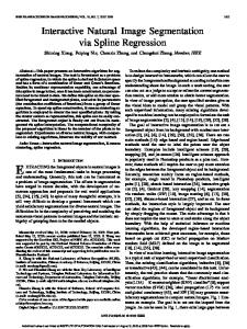
Jun 9, 2009 - the results of pixel classification (center), the original image marked with the ... In modern jargon, we call this interactive boosting (Freund and ...
Journal of Statistical Software
JSS
June 2009, Volume 30, Issue 10.
http://www.jstatsoft.org/
An Interactive Java Statistical Image Segmentation System: GemIdent Susan Holmes
Adam Kapelner
Peter P. Lee
Stanford University
Stanford Medical School
Stanford Medical School
Abstract Supervised learning can be used to segment/identify regions of interest in images using both color and morphological information. A novel object identification algorithm was developed in Java to locate immune and cancer cells in images of immunohistochemicallystained lymph node tissue from a recent study published by Kohrt et al. (2005). The algorithms are also showing promise in other domains. The success of the method depends heavily on the use of color, the relative homogeneity of object appearance and on interactivity. As is often the case in segmentation, an algorithm specifically tailored to the application works better than using broader methods that work passably well on any problem. Our main innovation is the interactive feature extraction from color images. We also enable the user to improve the classification with an interactive visualization system. This is then coupled with the statistical learning algorithms and intensive feedback from the user over many classification-correction iterations, resulting in a highly accurate and user-friendly solution. The system ultimately provides the locations of every cell recognized in the entire tissue in a text file tailored to be easily imported into R (Ihaka and Gentleman 1996; R Development Core Team 2009) for further statistical analyses. This data is invaluable in the study of spatial and multidimensional relationships between cell populations and tumor structure. This system is available at http://www.GemIdent.com/ together with three demonstration videos and a manual.
Keywords: interactive boosting, cell recognition, image segmentation, Java.
1. Introduction We start with an overview of current practices in image recognition and a short presentation of the clinical context that motivated this research, we then describe the software and the complete workflow involved, finally the last two sections present technical details and potential improvements. The interactive algorithm, although developed to solve a specific problem in
2
An Interactive Java Statistical Image Segmentation System: GemIdent
Figure 1: The original image (left), a mask superimposed on the original image showing the results of pixel classification (center), the original image marked with the centers of the oranges (right). histology, works on a wide variety of images. For instance, locating of oranges in a photograph of an orange grove (see Figure 1). Any image that has few relevant colors, such as green and orange in the above example, where the objects of interest vary little in shape, size, and color, can be analyzed using our algorithm. First, we will describe the application to cell recognition in microscopic images.
1.1. Previous research As emphasized in recent reviews (Ortiz de Solirzano et al. 1999; Mahalanobis et al. 1996; Wu et al. 1995, 1998; Yang and Parvin 2003; Gil et al. 2002; Fang et al. 2003; Kovalev et al. 2006), automated computer vision techniques applied to microscopy images are transforming the field of pathology. Not only can computerized vision techniques automate cell type recognition but they enable a more objective approach to cell classification providing at the same time a hierarchy of quantitative features measured on the images. Recent work on character recognition (Chakraborty 2003) shows how efficient interactivity can be in image recognition problems, with the user pointing out mistakes in real time, thus providing online improvement. In modern jargon, we call this interactive boosting (Freund and Schapire 1997). Current cell image analysis systems such as EBImage (Sklyar and Huber 2006) and Midas (Levenson 2006) or ImageJ (Collins 2007) do not provide these interactive visualization and correction features.
1.2. The specific context of breast cancer prognosis Kohrt et al. (2005) showed that breast cancer prognosis could be greatly improved by using immune population information from immunohistochemically-stained lymph nodes. To take this analysis a step further, we would like to detect and pinpoint the location of each and every cancer and immune cell in the high-resolution full-mount images of lymph nodes acquired via automated microscopy. This task is harder than classification of an entire slide as normal or abnormal as done in Maggioni et al. (2004) for instance. A typical tissue contains a variety of regions characteristic of cancer, immune cells, or both. It would not be possible for a histopathologist to identify and count all the cells of each type on such a slide. Even if a whole team of cell counters were available, the problems of subjectivity and bias on such a scale would discredit the results. It is very useful to have an automated
Journal of Statistical Software
3
Figure 2: The original image (left), a mask superimposed on the original image showing the results of pixel classification (center), the original image marked with the centers of the nuclei (right). system to identify and count cells objectively. Kohrt et al. (2005) also showed that T-cell and dendritic cell populations within axillary lymph nodes of patients with breast cancer are significantly decreased in patients who relapsed. No study thus far has examined the spatial variability in lymphocyte populations and phenotypes as related to lymph node-infiltrating tumor cells and clinical outcome. The location of tumordependent immune modulation has significant sequelæ, given the critical role of lymph nodes in activation of the immune response. This suggests that tissue architecture could yield clues to the workings of the immune system in breast cancer. This can be investigated through spatial analysis of different cell populations. The limiting step to date has been locating every cell.
1.3. GemIdent This algorithm has been engineered into the software package named GemIdent (Kapelner et al. 2007a,b). The distribution, implemented in Java, includes an easy-to-use GUI with four panels – color (or stain) training, phenotype training/retraining (see Figures 8, 10, and 11), classification, and data analysis (see Figure 13) with a final data output into a text file which is easy to input and analyse in R. The Java implementation ensures that full platform-independence is supported. In addition to supporting standard RGB images (in tiff or jpg format), the distribution also includes support for image sets derived from the Bacus Laboratories Incorporated Slide Scanner (BLISS, Bacus Laboratories, Inc.) and the CRI Nuance Multispectral Imager (CRI Inc., Woburn, MA). In this paper, we focus on the software itself, its use in conjunction with R and the developments which were engineered to analyze multispectral images where the chromatic markers (called chromagens) are separated a priori . Figure 2 shows GemIdent employed in the localization of cancer nuclei in a typical Kohrt (Kohrt et al. 2005) image. The algorithm internals are detailed in Section 2 but we give a brief summary here for potential users who do not need to know the technical details. Our procedure requires interactive training: the user defines the target objects sought from the images. In the breast cancer study, this would be the cancer nuclei themselves. The user must also provide examples of the “opposite” of the cancer nuclei, i.e. the “non-object” (NON). Figure 3 shows an excerpt from the training step. New images can be classified into cancer nuclei and non-cancer nuclei regions using a statistical
4
An Interactive Java Statistical Image Segmentation System: GemIdent
Figure 3: An example of training in a microscopic image of immunohistochemically stained lymph node. The cancer membranes are stained for Fast Red (displays maroon). There is a background nuclei counterstain that appears blue. The phenotype of interest are cancer cell nuclei. Training points for the nuclei appear as red diamonds and training points for the NON appear as green crosses. learning classifier (Hastie et al. 2001). Using simple geometric techniques, the centers of the cancer nuclei can then be located and an accurate count tabulated. The user can then return and examine the mistakes, correct them, and retrain the classifier. In this way a more accurate classifier is iteratively constructed. The process is repeated until the user is satisfied with the results. In Section 3 we detail a classification and analysis of an entire multispectrally-imaged Kohrt lymphnode, complete with screenshots of the software at each step.
2. Algorithm Image acquisition Any multiple wavelength set of images can be used, as long as they are completely aligned. In this example, the images were acquired via a modified CRI Nuance Multispectral Imager (CRI Inc., Woburn, MA). The acquisition was completely automated via an electronically controlled microscopy with an image decomposition into subimages. Multiple slides were sequentially scanned via an electronically controlled cartridge that feeds and retracts slides to and from the stage. The setup enables scanning of multiple slides with large histological samples (some being 10mm+ in diameter and spanning as many as 5, 000 subimages or stages) at 200X magnification. Each raw exposure is a collection of eight monochromatic images corresponding to the eight unique wavelength filters scanned (for information on dimension reduction in spectral imaging see Lee et al. 1990). The choice of eight is to ensure a complete span of the range of the visual spectrum but small enough to ensure a reasonable speed of image acquisition and avoid unwieldly amounts of data. These multispectral images are composed of 15-bit pixels whose values correspond to the optical density at that location. The files for each wavelength for each subimage or stage are typically TIF files of about 3MB each. Prior to whole-tissue scanning, a small representative image is taken that contains lucid ex-
Journal of Statistical Software
5
Figure 4: Example of a ring mask: c4 superimposed onto a typical cancer nuclei from the Kohrt images, white pixels designate the points which participate in the ring’s score. amples of each of the S chromagens. The user selects multiple examples of each of the S chromagens. This information is used to compute a “spectral library.” The same spectral library can then be used for every histological sample that is stained with the same chromagens. After whole-tissue scanning, the CRI Nuance Multispectral Imager (CRI Inc., Woburn, MA) combines the intermediate images using spectral unmixing algorithms to yield S orthogonal chromagen channel images. These “spectrally unmixed” images are also monochromatic and composed of 15-bit pixels whose values correspond to a pseudo-optical density. We use the spectrally unmixed images directly as score matrices, which we call Fs where s is the chromagen of interest. The program has been used with various scoring generation mechanisms and the quality of the statistical learning output has proved quite robust to these changes. Multispectral microscopy has the advantage of providing a clean separation of the chromagen signals.
Training phase 1. Interactive acquisition of the training sets for objects of interest. For each of the P phenotypes or categories of objects of interest, a training set is built: the user interactively chooses example points, t = (i, j), in the images where the phenotype is located forming the lists: T1+ , T2+ , . . . , TP+ . In addition, the user interactively chooses example points where none of the P phenotypes are located, i.e. the “NON” forming the list T − .
Learning phase 2. Feature definition: (a) Define a “ring”, cr , to be the 0/1 mask of the locus of pixels, t, r + � distance away from the center point to where � refers to the error inherent in discretizing a circle (see Figure 4). Generate a set of rings, for r ∈ {0, 1, 2, . . . , R} where R is the maximum radius of the largest phenotype to be identified and it can be modified by a multiplicative factor which controls the amount of additonal information beyond R to be included: C ≡ {c1 , c2 , . . . , cR }
6
An Interactive Java Statistical Image Segmentation System: GemIdent (b) For a point to = (io , jo ) in the training set and for a ring cr , create a “Ring Score,” `q,r , by summing the scores for all points in the mask: X Fs (to + t) `s,r (to ) = t ∈ cr
(c) Repeat for all rings in C and for all S score matrices to generate the observation record, Li of length S ×R by vectorizing `s,r and appending the categorical variable denoting the phenotype, p: � L(to ) = `1,1 , `1,2 , . . . , `1,R , `2,1 , `2,2 , . . . , `2,R , . . . . . . , `S,1 , `S,2 , . . . , `S,R , p (d) Now compute an observation record for each point t in the training sets for all phenotypes and for the ‘NON’ category. 3. Creation of a classifier: All observation vectors are concatenated row-wise into a training data matrix, and a supervised learning classifier that will be used to classify all phenotypes is created. In this implementation we use the statistical learning technique known as “Random Forests” developed by Breiman (2001) to automatically rank features among a large collection of candidates. This technique has been compared to a suite of other learning techniques in a cell recognition problem in Kovalev et al. (2006) who found it to be the best technique providing both the most accurate and the least variable of all the techniques compared. As all supervised learning techniques (Hastie et al. 2001), the method depends on the availability of a good training set of images where the pixels have already been classified into several groups. At this point, all previous data generated can be discarded. Most machine learning classifiers, including our version of Random Forests, provide information on which scores `q,r are important in the classification (see an example in Figure 9).
Classification phase 4. Pixel classification: For each image I to be classified, an observation record is created for each pixel (steps 2a and 2b), L(to ), and then evaluated by the classifier. The result is then stored in a binary matrix, with 1 coding for the phenotype and 0 for the opposite. There are P binary matrices, B1 , B2 , . . . , BP , (one for each phenotype): I
supervised learning classifier
−−−−−−−−−−−−−−−−−−−−−−−→ B1 , B2 , . . . , BP
To enhance speed, k pixels can be skipped at a time and the Bp ’s can be closed k times (dilated then eroded using a 4N mask, see Gonzalez et al. 2004) to fill in holes. 5. Post-processing Each pixel is now classified. Contiguously classified regions, called “blobs” hereon are post-processed in order to locate centers of the relevant objects, such as the middle of an orange or the cell nucleus.
Journal of Statistical Software
7
Figure 5: Left: Excerpt of Bcancer matrix. Right: The results of the centroid-finding algorithm superimposed on the marked image. Define the matrices C to hold centroid information: B1 , B2 , . . . , BP
blob analysis
−−−−−−−−−−−→ C1 , C2 , . . . , CP
There are many such algorithms for blob analysis. We used a simple one which we summarize below. For a more detailed description, see Appendix A. For an example of the results it produces, see Figure 5 A sample distribution of the training blob sizes is created by reconciling the user’s training points then counting the number of pixels in each blob using the floodfill algorithm. We calculated the 2nd percentile, 95th percentile, and the mean. For each blob obtained from the classification, we used those sample statistics to formulate a heuristic rule that discards those that are too small and quarantines those that are too large. Those that are too large are split up based on the mean blob size. To locate each blob’s centroid, the blob’s coordinates were averaged.
Additional training phase(s) 6. Retraining-reclassification iterations: After classification (and post-processing if desired), the results from the B’s and the C’s can be superimposed onto the original training image. The user can add false negatives (hence adding points to the Tp+ ’s) and add false positives (hence adding points to T − ). The observation records can then be regenerated, the supervised learning classifier can be relearned, and classification can be rerun with greater accuracy. This retrainingreclassification process can be repeated until the user is satisfied with the results.
3. A complete example Immunohistochemical staining (IHC) refers to the process of identifying proteins in cells of a slice of tissue through the specificity with which certain antibodies bind to special antigens
8
An Interactive Java Statistical Image Segmentation System: GemIdent
Figure 6: The tumor invaded lymph node as it appears through the microscope, at this resolution we can see the red zones which are Tumor invaded. present on (or inside of) the cell. Combining a stain called a chromagen with the antibodies allows visualization and reveals their localization within the field. IHC is thus widely used to discover in situ distributions of different types of cells. Until recently most of the data collection was done by manual cell counting. In this example we will show how different types of immune cells as well as cancer cells were detected and localized in large numbers using statistical learning for image segmentation. A lymphnode tissue section (see Figure 6) was stained for the folllowing markers by the following chromagens: CD1a targeting dendritic cells, 3, 30 −Diaminobenzidine (DAB); CD4 targeting T-cells, Ferangi Blue; and AE1/AE3 targeting cytokeratin within breast cancer cells, Vulcan Red. In addition, slides were stained with blue Hematoxylin to reveal all nuclei. The tissue was then imaged multispectrally (see “Image acquisition” in Section 2) and the set was loaded as a new project into GemIdent.
3.1. Selecting the training set When the image set is first opened, a training helper appears (see Figure 7). Each number represents the snapshots (called stages) captured individually by the system. The user then chooses a small, but representative number of images to compose the initial “training set.”
3.2. Initial training The user begins in the “phenotype training” tab and first enumerates the phenotypes being
Journal of Statistical Software
9
Figure 7: An assembly of all the individual stages in the complete scan. The parts of the images that we want to train and classify are indicated in green, the ones that will be discarded have red numbers, the green disks show the training set.
Figure 8: The pixels chosen as training points are shown as crosses. The color of the crosses indicates the training phenotype chosen.
10
An Interactive Java Statistical Image Segmentation System: GemIdent
sought and chooses an identifying color for each phenotype. Tumor cell nuclei were chosen to be green; T-cell nuclei, yellow; Dendritic cell nuclei, pink; and unspecified nuclei (called other_cell), orange (see left pane in Figure 8). The user then begins interactively selecting pixels that exemplify each phenotype as well as examples of pixels that do not represent any of the phenotypes (ie the “NON” pixels) by clicking on the image (see Section 2, Step 1). A magnification window with customizable zoom helps the user select precise pixels, allowing for a highly accurate training set. The current image being trained can be alternated by selecting from thumbnails representing the training set (see main, right, and bottom panels in Figure 8). In multispectral image sets, each individual chromagen signal can be customized (see the “Color Adjustment” dialog window in Figure 8). The display color can be chosen arbitrarily and the range of signal to be displayed can also be varied. In addition, chromagens can be flashed on/off. This is useful when training sets with phenotypes represented by chromagen colocalizations (none of the phenotypes in this example exhibit this property). There is also a rare event finder that searches the entire set for instances of rare markers or colocalizations (not shown).
3.3. Classification After specifying a training set for all phenotypes and the NON’s, the user transitions to the classification tab (not shown). Here, the user can customize the number of trees in the random forest classifier, number of CPUs to be utilized, which images to classify, and a few other options before classification. GemIdent then proceeds to creates a random forest (see Section 2, Steps 2 and 3). Upon completion, a graphic is displayed illustrating the importances of each feature in the classifier (see Figure 9). Then, every pixel is assigned a phenotype or put in the “NON” group by evaluating it in the random forest (see Section 2, Step 4). The output is zones or “blobs” of different phenotypes. Upon completion, the user can choose to resolve the blobs into centroids (see Section 2, Step 5), thus enabling cell counting and cell localization. After the centroids have been located, the program can evaluate its errors. The type I errors are shown in a small window and written to a summary file in the output directory: filename,Num_Dendritic_cells,Num_T_cells,Num_other_cells,Num_Tumor stage_0096,23,482,479,44 stage_0093,29,230,259,615 stage_0126,3,46,166,816 stage_0147,18,1203,907,81 ................... Error Rates Dendritic_cells 2.78 T_cells 4.35 other_cells 0.0 Tumor 7.34 Totals,922,85108,75457,27790
Journal of Statistical Software
11
Figure 9: Bar charts for interpreting the distance at which the chromagens influence the classifier. Each plot represents a chromagen with the x-axis indicating the ring score’s radius and the y-axis indicating relative importance (with the largest bar being the most important). The Hematoxylin was found to be very important at r ∈ [0, . . . , 5]. The forest learned that cancer cell nuclei, T-cell nuclei, and unspecific cell nuclei all have hematoxylin-rich centers. Ferangi Blue was found to be most important at r ∈ [4, . . . , 6] indicating that the classifier learned that the T-cells are positive at their membranes. Vulcan Red was found to be most important at r ∈ [6, . . . , 15] indicating that cancer cells are positive on their membranes and their diameter varies dramatically. DAB was found to be important at r ∈ [1, . . . , 6] indicating that dendritic cells appear devoid of a nucleus and vary in size. The user then transitions back to the “phenotype training” tab to view the results (see Figures 10 and 11).
3.4. Retraining GemIdent undoubtedly made mistakes during its initial classification and the user will wish to improve the results by retraining over the mistakes (see Section 2, Step 6). The software has many tools that aid the user in retraining:
12
An Interactive Java Statistical Image Segmentation System: GemIdent
Figure 10: After the training sets have been classified, the pixels in the different phenotypes appear as blobs. The result masks are overlaid atop the original image. Alpha sliders for pixel and centroid masks:
Figure 10 shows the pixel masks overlaid and Figure 11 shows the centroid masks overlaid atop the original image. Both screenshots include the “overlay adjustment” dialog box (top). The sliders in this dialog can be adjusted to vary the opacity of the mask. When the masks are translucent, the user can view the underlying tissue and the classification results simultaneously, and GemIdent’s errors can be located with ease. The “blink” checkboxes in the dialog box are used when the user feels translucent viewing does not adequately display both the tissue and the mask and wishes to flash the mask on/off. Localizing type I errors:
Points where the user trained positive for a phenotype, but after classification did not yield a nearby centroid, are called “type I errors.” GemIdent has an option to visualize these errors so the user can train over them (see Figure 12). Adding other images to the training set Images not specifically in the training set can be observed and if errors are found, they can be added to the training set. This ensures
Journal of Statistical Software
13
Figure 11: The cell centroids are marked by black stars filled with the relevant phenotype’s color. The result masks are overlaid atop the original image. that the training set becomes more representative of the entire image set, which is a type of boosting. GemIdent provides a convenient option where these images can be cycled through and perused quickly. After retraining, the image set can be reclassified and reviewed. The user can iterate until satisfied with the error rates.
3.5. Simple analyses and reporting The data analysis tab (see Figure 13) supports basic queries, displays histograms, and generates summary reports.
3.6. Data analysis with R During classification, the centroid data is written to a text file named after the particular phenotype they belong to with 5 columns: the stage number (which is the subimage to which the cell belonged), and the local and global X and Y coordinates. For instance, the file 99_4525D-Tumor.txt contains:
14
An Interactive Java Statistical Image Segmentation System: GemIdent
Figure 12: Type I errors are displayed surrounded by red circles.
Figure 13: The data analysis tab. The left panel displays the images currently in memory. By default, pixel and centroid results are loaded. The main window shows the result of a query asking for the distribution of distances from Tumor cells to their nearest T-cell neighbors. The open PDF document is the autogenerated report which includes a thumbnail view of the entire image set, counts and type I error rates for all phenotypes, as well as a transcript of the analyses performed.
Journal of Statistical Software
15
filename,locX,locY,globalX,globalY stage_0096,201,51,4040,13037 stage_0096,214,91,4053,13077 stage_0096,220,76,4059,13062 stage_0096,230,107,4069,13093 ....................... This data is easily read into R packages such as spatstat (Baddeley and Turner 2005) and transformed into an object of the ppp class. As in this short example: R> R> R> R> R> R> R> R> R> R> R> + + + + R> R> + + + R> R> + R> R> + R>
DCs