An Introduction to Recursive Partitioning Using the RPART Routines

An Introduction to Recursive Partitioning Using the RPART Routines Terry M. Therneau Elizabeth J. Atkinson Mayo Foundation January 11, 2011

Contents 1 Introduction

2

2 Notation

4

3 Building the tree 3.1 Splitting criteria . . . . . . . . . . . . . . . . . . . 3.2 Incorporating losses . . . . . . . . . . . . . . . . . 3.2.1 Generalized Gini index . . . . . . . . . . . . 3.2.2 Altered priors . . . . . . . . . . . . . . . . . 3.3 Example: Stage C prostate cancer (class method)

. . . . .

5 5 7 7 8 9

4 Pruning the tree 4.1 Definitions . . . . . . . . . . . . . . . . . . . . . . . . . . . . . . . . . 4.2 Cross-validation . . . . . . . . . . . . . . . . . . . . . . . . . . . . . . 4.3 Example: The Stochastic Digit Recognition Problem . . . . . . . . .

11 11 12 13

5 Missing data 5.1 Choosing the split . . . . . . . . . . . . . . . . . . . . . . . . . . . . 5.2 Surrogate variables . . . . . . . . . . . . . . . . . . . . . . . . . . . . 5.3 Example: Stage C prostate cancer (cont.) . . . . . . . . . . . . . . .

16 16 17 18

6 Further options 6.1 Program options . . . . . . . . . . . . . . . . . . . . . . . . . . . . . 6.2 Example: Consumer Report Auto Data . . . . . . . . . . . . . . . . 6.3 Example: Kyphosis data . . . . . . . . . . . . . . . . . . . . . . . . .

20 20 22 25

1

. . . . .

. . . . .

. . . . .

. . . . .

. . . . .

. . . . .

. . . . .

. . . . .

. . . . .

7 Regression 7.1 Definition . . . . . . . . . . . . . . . . . . . . . . . . . . . . . . . . . 7.2 Example: Consumer Report car data . . . . . . . . . . . . . . . . . . 7.3 Example: Stage C data (anova method) . . . . . . . . . . . . . . . .

28 28 29 34

8 Poisson regression 8.1 Definition . . . . . . . . . . . . . . 8.2 Improving the method . . . . . . . 8.3 Example: solder data . . . . . . . . 8.4 Example: Stage C Prostate cancer, 8.5 Open issues . . . . . . . . . . . . .

35 35 36 37 40 45

. . . . . . . . . . . . . . . . . . . . . . . . . . . . . . survival method . . . . . . . . . .

. . . . .

. . . . .

. . . . .

. . . . .

. . . . .

. . . . .

. . . . .

. . . . .

. . . . .

9 Plotting options

46

10 Other functions

50

11 Relation to other programs 11.1 CART . . . . . . . . . . . . . . . . . . . . . . . . . . . . . . . . . . . 11.2 Tree . . . . . . . . . . . . . . . . . . . . . . . . . . . . . . . . . . . .

50 50 51

12 Test Cases 12.1 Classification . . . . . . . . . . . . . . . . . . . . . . . . . . . . . . .

52 52

13 User written rules 13.1 Anova . . . . . . . . . . . . 13.2 Smoothed anova . . . . . . 13.3 Classification with an offset 13.4 Cost-complexity pruning . .

55 56 60 62 65

. . . .

. . . .

. . . .

14 Source

1

. . . .

. . . .

. . . .

. . . .

. . . .

. . . .

. . . .

. . . .

. . . .

. . . .

. . . .

. . . .

. . . .

. . . .

. . . .

. . . .

. . . .

. . . .

. . . .

. . . .

66

Introduction

This document is an update of a technical report written several years ago at Stanford [6], and is intended to give a short overview of the methods found in the rpart routines, which implement many of the ideas found in the CART (Classification and Regression Trees) book and programs of Breiman, Friedman, Olshen and Stone [1]. Because CART is the trademarked name of a particular software implementation of these ideas, and tree has been used for the S-plus routines of Clark and Pregibon ∼[3] a different acronym — Recursive PARTitioning or rpart — was chosen.

2

24 revived 144 not revived H HH   HH   HH   HH 

X1 = 1 22 / 13   

X2 = 1 20 / 5

X1 =2, 3 or 4 2 / 131 H HH  HH 

H HH H H

X2 =2 or 3 2/8

X3 =1 2 / 31

X3 =2 or 3 0 / 100

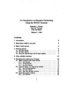
Figure 1: Revival data

The rpart programs build classification or regression models of a very general structure using a two stage procedure; the resulting models can be represented as binary trees. An example is some preliminary data gathered at Stanford on revival of cardiac arrest patients by paramedics. The goal is to predict which patients are revivable in the field on the basis of fourteen variables known at or near the time of paramedic arrival, e.g., sex, age, time from attack to first care, etc. Since some patients who are not revived on site are later successfully resuscitated at the hospital, early identification of these “recalcitrant” cases is of considerable clinical interest. The resultant model separated the patients into four groups as shown in figure 1, where X1 = initial heart rhythm 1= VF/VT 2=EMD 3=Asystole 4=Other X2 = initial response to defibrillation 1=Improved 2=No change 3=Worse X3 = initial response to drugs 1=Improved 2=No change 3=Worse The other 11 variables did not appear in the final model. This procedure seems to work especially well for variables such as X1 , where there is a definite ordering, but spacings are not necessarily equal. The tree is built by the following process: first the single variable is found which best splits the data into two groups (‘best’ will be defined later). The data is 3

separated, and then this process is applied separately to each sub-group, and so on recursively until the subgroups either reach a minimum size (5 for this data) or until no improvement can be made. The resultant model is, with a certainty, too complex, and the question arises as it does with all stepwise procedures of when to stop. The second stage of the procedure consists of using cross-validation to trim back the full tree. In the medical example above the full tree had ten terminal regions. A cross validated estimate of risk was computed for a nested set of subtrees; this final model was that subtree with the lowest estimate of risk.

2

Notation

The partitioning method can be applied to many different kinds of data. We will start by looking at the classification problem, which is one of the more instructive cases (but also has the most complex equations). The sample population consists of n observations from C classes. A given model will break these observations into k terminal groups; to each of these groups is assigned a predicted class. In an actual application, most parameters will be estimated from the data, such estimates are given by ≈ formulae. πi

i = 1, 2, ..., C

prior probabilities of each class

L(i, j)

i = 1, 2, ..., C Loss matrix for incorrectly classifying an i as a j. L(i, i) ≡ 0

A

some node of the tree Note that A represents both a set of individuals in the sample data, and, via the tree that produced it, a classification rule for future data.

τ (x)

true class of an observation x, where x is the vector of predictor variables

τ (A)

the class assigned to A, if A were to be taken as a final node

ni , nA

number of observations in the sample that are class i, number of obs in node A

P (A)

probability of A (for future observations) 4

P

p(i|A)

R(A)

R(T )

πi P {x ∈ A | τ (x) = i} = C Pi=1 C ≈ i=1 πi niA /ni

P {τ (x) = i | x ∈ A} (for future observations) = πi P {x ∈ A | τ (x) = i}/P {x ∈ A} P ≈ πi (niA /ni )/ πi (niA /ni ) risk of A P = C i=1 p(i|A)L(i, τ (A)) where τ (A) is chosen to minimize this risk

risk of a model (or tree) T P = kj=1 P (Aj )R(Aj ) where Aj are the terminal nodes of the tree

If L(i, j) = 1 for all i = 6 j, and we set the prior probabilities π equal to the observed class frequencies in the sample then p(i|A) = niA /nA and R(T ) is the proportion misclassified.

3 3.1

Building the tree Splitting criteria

If we split a node A into two sons AL and AR (left and right sons), we will have P (AL )r(AL ) + P (AR )r(AR ) ≤ P (A)r(A) (this is proven in [1]). Using this, one obvious way to build a tree is to choose that split which maximizes ∆r, the decrease in risk. There are defects with this, however, as the following example shows. Suppose losses are equal and that the data is 80% class 1’s, and that some trial split results in AL being 54% class 1’s and AR being 100% class 1’s. Since the minimum risk prediction for both the left and right son is τ (AL ) = τ (AR ) = 1, this split will have ∆r = 0, yet scientifically this is a very informative division of the sample. In real data with such a majority, the first few splits very often can do no better than this. A more serious defect is that the risk reduction is essentially linear. If there were two competing splits, one separating the data into groups of 85% and 50% purity 5

1.0 0.6 0.4

Scaled Impurity

0.8

0.6 0.4 0.2

Impurity

Gini criteria Information

0.0

0.0

0.2

Gini criteria Information

0.0

0.2

0.4

0.6

0.8

1.0

0.0

P

0.2

0.4

0.6

0.8

1.0

P

Figure 2: Comparison of Gini and Information indices

respectively, and the other into 70%-70%, we would usually prefer the former, if for no other reason than because it better sets things up for the next splits. One way around both of these problems is to use lookahead rules; but these are computationally very expensive. Instead rpart uses one of several measures of impurity, or diversity, of a node. Let f be some impurity function and define the impurity of a node A as I(A) =

C X

f (piA )

i=1

where piA is the proportion of those in A that belong to class i for future samples. Since we would like I(A) =0 when A is pure, f must be concave with f (0) = f (1) = 0. Two candidates for f are the information index f (p) = −p log(p) and the Gini index f (p) = p(1 − p). We then use that split with maximal impurity reduction ∆I = p(A)I(A) − p(AL )I(AL ) − p(AR )I(AR ) The two impurity functions are plotted in figure (2), with the second plot scaled so that the maximum for both measures is at 1. For the two class problem the measures differ only slightly, and will nearly always choose the same split point.

6

Another convex criteria not quite of the above class is twoing for which I(A) = min [f (pC1 ) + f (pC2 )] C1 C2

where C1 ,C2 is some partition of the C classes into two disjoint sets. If C = 2 twoing is equivalent to the usual impurity index for f . Surprisingly, twoing can be calculated almost as efficiently as the usual impurity index. One potential advantage of twoing is that the output may give the user additional insight concerning the structure of the data. It can be viewed as the partition of C into two superclasses which are in some sense the most dissimilar for those observations in A. For certain problems there may be a natural ordering of the response categories (e.g. level of education), in which case ordered twoing can be naturally defined, by restricting C1 to be an interval [1, 2, . . . , k] of classes. Twoing is not part of rpart.

3.2

Incorporating losses

One salutatory aspect of the risk reduction criteria not found in the impurity measures is inclusion of the loss function. Two different ways of extending the impurity criteria to also include losses are implemented in CART, the generalized Gini index and altered priors. The rpart software implements only the altered priors method. 3.2.1

Generalized Gini index

The Gini index has the following interesting interpretation. Suppose an object is selected at random from one of C classes according to the probabilities (p1 , p2 , ..., pC ) and is randomly assigned to a class using the same distribution. The probability of misclassification is XX i

j6=i

pi pj =

XX i

j

pi pj −

X

p2i =

i

X i

1 − p2i = Gini index for p

Let L(i, j) be the loss of assigning class j to an object which actually belongs to class PP i. The expected cost of misclassification is L(i, j)pi pj . This suggests defining a generalized Gini index of impurity by G(p) =

XX i

L(i, j)pi pj

j

The corresponding splitting criterion appears to be promising for applications involving variable misclassification costs. But there are several reasonable objections to it. First, G(p) is not necessarily a concave function of p, which was the motivating

7

factor behind impurity measures. More seriously, G symmetrizes the loss matrix before using it. To see this note that G(p) = (1/2)

XX

[L(i, j) + L(j, i)] pi pj

In particular, for two-class problems, G in effect ignores the loss matrix. 3.2.2

Altered priors

Remember the definition of R(A) R(A) ≡ =

C X

i=1 C X

piA L(i, τ (A)) πi L(i, τ (A))(niA /ni )(n/nA )

i=1

˜ be such that Assume there exists π ˜ and L ˜ j) = πi L(i, j) π ˜i L(i,

∀i, j ∈ C

˜ is proportional to Then R(A) is unchanged under the new losses and priors. If L the zero-one loss matrix then the priors π ˜ should be used in the splitting criteria. This is possible only if L is of the form L(i, j) = in which case

(

Li i 6= j 0 i=j

π i Li π ˜i = P j π j Lj

This is always possible when C = 2, and hence altered priors are exact for the two class problem. For arbitrary loss matrix of dimension C > 2, rpart uses the above P formula with Li = j L(i, j). A second justification for altered priors is this. An impurity index I(A) = P f (pi ) has its maximum at p1 = p2 = . . . = pC = 1/C. If a problem had, for instance, a misclassification loss for class 1 which was twice the loss for a class 2 or 3 observation, one would wish I(A) to have its maximum at p1 =1/5, p2 = p3 =2/5, since this is the worst possible set of proportions on which to decide a node’s class. The altered priors technique does exactly this, by shifting the pi . Two final notes 8

grade< 2.5 |

g2< 13.2 No

g2>=17.91

ploidy=ab

g2>=11.85 g2< 11

Prog

No age>=62.5 Prog No

Prog

No

Prog

Figure 3: Classification tree for the Stage C data

• When altered priors are used, they affect only the choice of split. The ordinary losses and priors are used to compute the risk of the node. The altered priors simply help the impurity rule choose splits that are likely to be “good” in terms of the risk. • The argument for altered priors is valid for both the gini and information splitting rules.

3.3

Example: Stage C prostate cancer (class method)

This first example is based on a data set of 146 stage C prostate cancer patients [5]. The main clinical endpoint of interest is whether the disease recurs after initial surgical removal of the prostate, and the time interval to that progression (if any). The endpoint in this example is status, which takes on the value 1 if the disease has progressed and 0 if not. Later we’ll analyze the data using the exp method, which will take into account time to progression. A short description of each of the variables is listed below. The main predictor variable of interest in this study was DNA ploidy, as determined by flow cytometry. For diploid and tetraploid tumors, the flow cytometric method was also able to estimate the percent of tumor cells in a G2 (growth) stage of their cell cycle; G2 % is systematically missing for most aneuploid tumors. 9

The variables pgtime pgstat age eet ploidy g2 grade gleason

in the data set are time to progression, or last follow-up free of progression status at last follow-up (1=progressed, 0=censored) age at diagnosis early endocrine therapy (1=no, 0=yes) diploid/tetraploid/aneuploid DNA pattern % of cells in G2 phase tumor grade (1-4) Gleason grade (3-10)

The model is fit by using the rpart function. The first argument of the function is a model formula, with the ∼ symbol standing for “is modeled as”. The print function gives an abbreviated output, as for other S models. The plot and text command plot the tree and then label the plot, the result is shown in figure 3. > progstat cfit print(cfit) node), split, n, loss, yval, (yprob) * denotes terminal node 1) root 146 54 No ( 0.6301 0.3699 ) 2) grade2.5 85 40 Prog ( 0.4706 0.5294 ) 6) g211.845 7 1 No ( 0.8571 0.1429 ) * 25) g213.2 45 17 Prog ( 0.3778 0.6222 ) 14) g2>17.91 22 8 No ( 0.6364 0.3636 ) 28) age>62.5 15 4 No ( 0.7333 0.2667 ) * 29) age text(cfit)

• The creation of a labeled factor variable as the response improves the labeling of the printout. 10

• We have explicitly directed the routine to treat progstat as a categorical variable by asking for method=’class’. (Since progstat is a factor this would have been the default choice). Since no optional classification parameters are specified the routine will use the Gini rule for splitting, prior probabilities that are proportional to the observed data frequencies, and 0/1 losses. • The child nodes of node x are always 2x and 2x + 1, to help in navigating the printout (compare the printout to figure 3). • Other items in the list are the definition of the split used to create a node, the number of subjects at the node, the loss or error at the node (for this example, with proportional priors and unit losses this will be the number misclassified), and the predicted class for the node. • * indicates that the node is terminal. • Grades 1 and 2 go to the left, grades 3 and 4 go to the right. The tree is arranged so that the branches with the largest “average class” go to the right.

4 4.1

Pruning the tree Definitions

We have built a complete tree, possibly quite large and/or complex, and must now decide how much of that model to retain. In stepwise regression, for instance, this issue is addressed sequentially and the fit is stopped when the F test fails to achieve some level α. Let T1 , T2 ,....,Tk be the terminal nodes of a tree T. Define |T | = number of terminal nodes P risk of T = R(T ) = ki=1 P (Ti )R(Ti )

In comparison to regression, |T | is analogous to the degrees of freedom and R(T ) to the residual sum of squares. Now let α be some number between 0 and ∞ which measures the ’cost’ of adding another variable to the model; α will be called a complexity parameter. Let R(T0 ) be the risk for the zero split tree. Define Rα (T ) = R(T ) + α|T | to be the cost for the tree, and define Tα to be that subtree of the full model which has minimal cost. Obviously T0 = the full model and T∞ = the model with no splits at all. The following results are shown in [1]. 11

1. If T1 and T2 are subtrees of T with Rα (T1 ) = Rα (T2 ), then either T1 is a subtree of T2 or T2 is a subtree of T1 ; hence either |T1 | < |T2 | or |T2 | < |T1 |. 2. If α > β then either Tα = Tβ or Tα is a strict subtree of Tβ . 3. Given some set of numbers α1 , α2 , . . . , αm ; both Tα1 , . . . , Tαm and R(Tα1 ), . . ., R(Tαm ) can be computed efficiently. Using the first result, we can uniquely define Tα as the smallest tree T for which Rα (T ) is minimized. Since any sequence of nested trees based on T has at most |T | members, result 2 implies that all possible values of α can be grouped into m intervals, m ≤ |T | I1 = [0, α1 ] I2 = (α1 , α2 ] .. . Im = (αm−1 , ∞] where all α ∈ Ii share the same minimizing subtree.

4.2

Cross-validation

Cross-validation is used to choose a best value for α by the following steps: 1. Fit the full model on the data set compute I1 , I2 , ..., Im set β1 = 0 √ β2 = α1 α2 √ β3 = α2 α3 .. . √ βm−1 = αm−2 αm−1 βm = ∞ each βi is a ‘typical value’ for its Ii 2. Divide the data set into s groups G1 , G2 , ..., Gs each of size s/n, and for each group separately: • fit a full model on the data set ‘everyone except Gi ’ and determine Tβ1 , Tβ2 , ..., Tβm for this reduced data set, • compute the predicted class for each observation in Gi , under each of the models Tβj for 1 ≤ j ≤ m, 12

• from this compute the risk for each subject. 3. Sum over the Gi to get an estimate of risk for each βj . For that β (complexity parameter) with smallest risk compute Tβ for the full data set, this is chosen as the best trimmed tree. In actual practice, we may use instead the 1-SE rule. A plot of β versus risk often has an initial sharp drop followed by a relatively flat plateau and then a slow rise. The choice of β among those models on the plateau can be essentially random. To avoid this, both an estimate of the risk and its standard error are computed during the cross-validation. Any risk within one standard error of the achieved minimum is marked as being equivalent to the minimum (i.e. considered to be part of the flat plateau). Then the simplest model, among all those “tied” on the plateau, is chosen. In the usual definition of cross-validation we would have taken s = n above, i.e., each of the Gi would contain exactly one observation, but for moderate n this is computationally prohibitive. A value of s = 10 has been found to be sufficient, but users can vary this if they wish. In Monte-Carlo trials, this method of pruning has proven very reliable for screening out ‘pure noise’ variables in the data set.

4.3

Example: The Stochastic Digit Recognition Problem

This example is found in section 2.6 of [1], and used as a running example throughout much of their book. Consider the segments of an unreliable digital readout

1 2

4

5

3

6 7

where each light is correct with probability 0.9, e.g., if the true digit is a 2, the lights 1, 3, 4, 5, and 7 are on with probability 0.9 and lights 2 and 6 are on with probability 0.1. Construct test data where Y ∈ {0, 1, ..., 9}, each with proportion 1/10 and the Xi , i = 1, . . . , 7 are i.i.d. Bernoulli variables with parameter depending on Y. 13

x.7>=0.5 |

x.4< 0.5

x.3>=0.5

x.1>=0.5

x.6< 0.5

x.4< 0.5

5

2

6

x.1< 0.5

1

7

x.1< 0.5

4

9

x.5< 0.5 0 3

8

Figure 4: Optimally pruned tree for the stochastic digit recognition data

X8 − X24 are generated as i.i.d bernoulli P {Xi = 1} = .5, and are independent of Y. They correspond to imbedding the readout in a larger rectangle of random lights. A sample of size 200 was generated accordingly and the procedure applied using the gini index (see 3.2.1) to build the tree. The S-plus code to compute the simulated data and the fit are shown below. > n y temp lights temp1 temp1 temp2 x temp3 dfit printcp(dfit) Classification tree: rpart(formula = y ∼ x, method = "class", control = temp3) Variables actually used in tree construction: [1] x.1 x.10 x.12 x.13 x.15 x.19 x.2 x.20 x.22 x.3

x.4

x.5

x.6

x.7

Root node error: 180/200 = 0.9

1 2 3 4 5 6 7 8 9 10 11 12

CP nsplit rel error 0.1055556 0 1.00000 0.0888889 2 0.79444 0.0777778 3 0.70556 0.0666667 5 0.55556 0.0555556 8 0.36111 0.0166667 9 0.30556 0.0111111 11 0.27222 0.0083333 12 0.26111 0.0055556 16 0.22778 0.0027778 27 0.16667 0.0013889 31 0.15556 0.0000000 35 0.15000

xerror 1.09444 1.01667 0.90556 0.75000 0.56111 0.36111 0.37778 0.36111 0.35556 0.34444 0.36667 0.36667

xstd 0.0095501 0.0219110 0.0305075 0.0367990 0.0392817 0.0367990 0.0372181 0.0367990 0.0366498 0.0363369 0.0369434 0.0369434

> fit9 plot(fit9, branch=.3, compress=T) > text(fit9)

This table differs from that in section 3.5 of [1] in several ways, the last two of which are somewhat important. • The actual values are different, of course, because of different random number generators in the two runs. • The table is printed from the smallest tree (no splits) to the largest one (28 15

x.8

splits). We find it easier to compare one tree to another when they start at the same place. • The number of splits is listed, rather than the number of nodes. The number of nodes is always 1 + the number of splits. • For easier reading, the error columns have been scaled so that the first node has an error of 1. Since in this example the model with no splits must make 180/200 misclassifications, multiply columns 3-5 by 180 to get a result in terms of absolute error. (Computations are done on the absolute error scale, and printed on relative scale). • The complexity parameter column has been similarly scaled. Looking at the table, we see that the best tree has 10 terminal nodes (9 splits), based on cross-validation. This subtree is extracted with call to prune and saved in fit9. The pruned tree is shown in figure 4. Two options have been used in the plot. The compress option tries to narrow the printout by vertically overlapping portions of the plot. (It has only a small effect on this particular dendrogram). The branch option controls the shape of the branches that connect a node to its children. The section on plotting (9) will discuss this and other options in more detail. The largest tree, with 35 terminal nodes, correctly classifies 170/200 = 85% of the observations, but uses several of the random predictors in doing so and seriously overfits the data. If the number of observations per terminal node (minbucket) had been set to 1 instead of 2, then every observation would be classified correctly in the final model, many in terminal nodes of size 1.

5 5.1

Missing data Choosing the split

Missing values are one of the curses of statistical models and analysis. Most procedures deal with them by refusing to deal with them – incomplete observations are tossed out. Rpart is somewhat more ambitious. Any observation with values for the dependent variable and at least one independent variable will participate in the modeling. The quantity to be maximized is still ∆I = p(A)I(A) − p(AL )I(AL ) − p(AR )I(AR ) The leading term is the same for all variables and splits irrespective of missing data, but the right two terms are somewhat modified. Firstly, the impurity indices 16

I(AR ) and I(AL ) are calculated only over the observations which are not missing a particular predictor. Secondly, the two probabilities p(AL ) and p(AR ) are also calculated only over the relevant observations, but they are then adjusted so that they sum to p(A). This entails some extra bookkeeping as the tree is built, but ensures that the terminal node probabilities sum to 1. In the extreme case of a variable for which only 2 observations are non-missing, the impurity of the two sons will both be zero when splitting on that variable. Hence ∆I will be maximal, and this ‘almost all missing’ coordinate is guaranteed to be chosen as best; the method is certainly flawed in this extreme case. It is difficult to say whether this bias toward missing coordinates carries through to the non-extreme cases, however, since a more complete variable also affords for itself more possible values at which to split.

5.2

Surrogate variables

Once a splitting variable and a split point for it have been decided, what is to be done with observations missing that variable? One approach is to estimate the missing datum using the other independent variables; rpart uses a variation of this to define surrogate variables. As an example, assume that the split (age summary(cfit,cp=.06) Node number 1: 146 observations, complexity param=0.1049 predicted class= No expected loss= 0.3699 class counts: 92 54 probabilities: 0.6301 0.3699 left son=2 (61 obs) right son=3 (85 obs) Primary splits: grade < 2.5 to the left, improve=10.360, (0 missing)

18

gleason < 5.5 to ploidy splits as g2 < 13.2 to age < 58.5 to Surrogate splits: gleason < 5.5 to ploidy splits as g2 < 9.945 to age < 66.5 to

the left, improve= 8.400, (3 missing) LRR, improve= 7.657, (0 missing) the left, improve= 7.187, (7 missing) the right, improve= 1.388, (0 missing) the left, agree=0.8630, (0 split) LRR, agree=0.6438, (0 split) the left, agree=0.6301, (0 split) the right, agree=0.5890, (0 split)

Node number 2: 61 observations predicted class= No expected loss= 0.1475 class counts: 52 9 probabilities: 0.8525 0.1475 Node number 3: 85 observations, complexity param=0.1049 predicted class= Prog expected loss= 0.4706 class counts: 40 45 probabilities: 0.4706 0.5294 left son=6 (40 obs) right son=7 (45 obs) Primary splits: g2 < 13.2 to the left, improve=2.1780, (6 missing) ploidy splits as LRR, improve=1.9830, (0 missing) age < 56.5 to the right, improve=1.6600, (0 missing) gleason < 8.5 to the left, improve=1.6390, (0 missing) eet < 1.5 to the right, improve=0.1086, (1 missing) Surrogate splits: ploidy splits as LRL, agree=0.9620, (6 split) age < 68.5 to the right, agree=0.6076, (0 split) gleason < 6.5 to the left, agree=0.5823, (0 split) . . .

• There are 54 progressions (class 1) and 94 non-progressions, so the first node has an expected loss of 54/146 ≈ 0.37. (The computation is this simple only for the default priors and losses). • Grades 1 and 2 go to the left, grades 3 and 4 to the right. The tree is arranged so that the “more severe” nodes go to the right. • The improvement is n times the change in impurity index. In this instance, the largest improvement is for the variable grade, with an improvement of 10.36. The next best choice is Gleason score, with an improvement of 8.4. 19

The actual values of the improvement are not so important, but their relative size gives an indication of the comparative utility of the variables. • Ploidy is a categorical variable, with values of diploid, tetraploid, and aneuploid, in that order. (To check the order, type table(stagec$ploidy)). All three possible splits were attempted: aneuploid+diploid vs. tetraploid, aneuploid+tetraploid vs. diploid, and aneuploid vs. diploid + tetraploid. The best split sends diploid to the right and the others to the left. • The 2 by 2 table of diploid/non-diploid vs grade= 1-2/3-4 has 64% of the observations on the diagonal. diploid tetraploid aneuploid

1-2 38 22 1

3-4 29 46 10

• For node 3, the primary split variable is missing on 6 subjects. All 6 are split based on the first surrogate, ploidy. Diploid and aneuploid tumors are sent to the left, tetraploid to the right. As a surrogate, eet was no better than 45/85 (go with the majority), and was not retained. Diploid/aneuploid Tetraploid

6

g2 < 13.2 71 3

g2 > 13.2 1 64

Further options

6.1

Program options

The central fitting function is rpart, whose main arguments are • formula: the model formula, as in lm and other S model fitting functions. The right hand side may contain both continuous and categorical (factor) terms. If the outcome y has more than two levels, then categorical predictors must be fit by exhaustive enumeration, which can take a very long time. • data, weights, subset: as for other S models. Weights are not yet supported, and will be ignored if present. • method: the type of splitting rule to use. Options at this point are classification, anova, Poisson, and exponential.

20

• parms: a list of method specific optional parameters. For classification, the list can contain any of: the vector of prior probabilities (component prior), the loss matrix (component loss) or the splitting index (component split). The priors must be positive and sum to 1. The loss matrix must have zeros on the diagonal and positive off-diagonal elements. The splitting index can be ‘gini’ or ‘information’. • na.action: the action for missing values. The default action for rpart is na.rpart, this default is not overridden by the options(na.action) global option. The default action removes only those rows for which either the response y or all of the predictors are missing. This ability to retain partially missing observations is perhaps the single most useful feature of rpart models. • control: a list of control parameters, usually the result of the rpart.control function. The list must contain – minsplit: The minimum number of observations in a node for which the routine will even try to compute a split. The default is 20. This parameter can save computation time, since smaller nodes are almost always pruned away by cross-validation. – minbucket: The minimum number of observations in a terminal node. This defaults to minsplit/3. – maxcompete: It is often useful in the printout to see not only the variable that gave the best split at a node, but also the second, third, etc best. This parameter controls the number that will be printed. It has no effect on computational time, and a small effect on the amount of memory used. The default is 4. – xval: The number of cross-validations to be done. Usually set to zero during exploratory phases of the analysis. A value of 10, for instance, increases the compute time to 11-fold over a value of 0. – maxsurrogate: The maximum number of surrogate variables to retain at each node. (No surrogate that does worse than “go with the majority” is printed or used). Setting this to zero will cut the computation time in half, and set usesurrogate to zero. The default is 5. Surrogates give different information than competitor splits. The competitor list asks “which other splits would have as many correct classifications”, surrogates ask “which other splits would classify the same subjects in the same way”, which is a harsher criteria. – usesurrogate: A value of usesurrogate=2, the default, splits subjects in the way described previously. This is similar to CART. If the value is 0, 21

then a subject who is missing the primary split variable does not progress further down the tree. A value of 1 is intermediate: all surrogate variables except “go with the majority” are used to send a case further down the tree. – cp: The threshold complexity parameter. The complexity parameter cp is, like minsplit, an advisory parameter, but is considerably more useful. It is specified according to the formula Rcp (T ) ≡ R(T ) + cp ∗ |T | ∗ R(T1 ) where T1 is the tree with no splits, |T | is the number of splits for a tree, and R is the risk. This scaled version is much more user friendly than the original CART formula (4.1) since it is unitless. A value of cp=1 will always result in a tree with no splits. For regression models (see next section) the scaled cp has a very direct interpretation: if any split does not increase the overall R2 of the model by at least cp (where R2 is the usual linear-models definition) then that split is decreed to be, a priori, not worth pursuing. The program does not split said branch any further, and saves considerable computational effort. The default value of .01 has been reasonably successful at ‘pre-pruning’ trees so that the cross-validation step need only remove 1 or 2 layers, but it sometimes overprunes, particularly for large data sets.

6.2

Example: Consumer Report Auto Data

A second example using the class method demonstrates the outcome for a response with multiple (> 2) categories. We also explore the difference between Gini and information splitting rules. The dataset cu.summary contains a collection of variables from the April, 1990 Consumer Reports summary on 117 cars. For our purposes, car Reliability will be treated as the response. The variables are: Reliability Price Country Mileage Type

an ordered factor (contains NAs): Much worse < worse < average < better < Much Better numeric: list price in dollars, with standard equipment factor: country where car manufactured numeric: gas mileage in miles/gallon, contains NAs factor: Small, Sporty, Compact, Medium, Large, Van

In the analysis we are treating reliability as an unordered outcome. Nodes potentially can be classified as Much worse, worse, average, better, or Much better, though there are none that are labelled as just “better”. The 32 cars with missing 22

Country=dghij

Country=dghij

|

|

Type=e Type=bcef

Much better 0/0/3/3/21

Type=e

Type=bcf Much worse 7/0/2/0/0 Country=gj average 7/4/16/0/0 worse average 4/6/1/3/00/2/4/2/0

Country=gj

Much better 0/0/3/3/21

worse average 4/6/1/3/00/2/4/2/0 Much worse average 7/0/2/0/07/4/16/0/0

Figure 5: Displays the rpart-based model relating automobile Reliability to car type, price, and country of origin. The figure on the left uses the gini splitting index and the figure on the right uses the information splitting index.

response (listed as NA) were not used in the analysis. Two fits are made, one using the Gini index and the other the information index. > fit1 fit2 par(mfrow=c(1,2)) > plot(fit1); text(fit1,use.n=T,cex=.9) > plot(fit2); text(fit2,use.n=T,cex=.9)

The first two nodes from the Gini tree are Node number 1: 85 observations, complexity param=0.3051 predicted class= average expected loss= 0.6941 class counts: 18 12 26 8 21 probabilities: 0.2118 0.1412 0.3059 0.0941 0.2471 left son=2 (58 obs) right son=3 (27 obs) Primary splits:

23

Country Type Price Mileage

splits as splits as < 11970 to < 24.5 to

---LRRLLLL, improve=15.220, (0 missing) RLLRLL, improve= 4.288, (0 missing) the right, improve= 3.200, (0 missing) the left, improve= 2.476, (36 missing)

Node number 2: 58 observations, complexity param=0.08475 predicted class= average expected loss= 0.6034 class counts: 18 12 23 5 0 probabilities: 0.3103 0.2069 0.3966 0.0862 0.0000 left son=4 (9 obs) right son=5 (49 obs) Primary splits: Type splits as RRRRLR, improve=3.187, (0 missing) Price < 11230 to the left, improve=2.564, (0 missing) Mileage < 24.5 to the left, improve=1.802, (30 missing) Country splits as ---L--RLRL, improve=1.329, (0 missing)

The fit for the information splitting rule is Node number 1: 85 observations, complexity param=0.3051 predicted class= average expected loss= 0.6941 class counts: 18 12 26 8 21 probabilities: 0.2118 0.1412 0.3059 0.0941 0.2471 left son=2 (58 obs) right son=3 (27 obs) Primary splits: Country splits as ---LRRLLLL, improve=38.540, (0 missing) Type splits as RLLRLL, improve=11.330, (0 missing) Price < 11970 to the right, improve= 6.241, (0 missing) Mileage < 24.5 to the left, improve= 5.548, (36 missing) Node number 2: 58 observations, complexity param=0.0678 predicted class= average expected loss= 0.6034 class counts: 18 12 23 5 0 probabilities: 0.3103 0.2069 0.3966 0.0862 0.0000 left son=4 (36 obs) right son=5 (22 obs) Primary splits: Type splits as RLLRLL, improve=9.281, (0 missing) Price < 11230 to the left, improve=5.609, (0 missing) Mileage < 24.5 to the left, improve=5.594, (30 missing) Country splits as ---L--RRRL, improve=2.891, (0 missing) Surrogate splits: Price < 10970 to the right, agree=0.8793, (0 split) Country splits as ---R--RRRL, agree=0.7931, (0 split)

The first 3 countries (Brazil, England, France) had only one or two cars in the listing, all of which were missing the reliability variable. There are no entries 24

for these countries in the first node, leading to the − symbol for the rule. The information measure has larger “improvements”, consistent with the difference in scaling between the information and Gini criteria shown in figure 2, but the relative merits of different splits are fairly stable. The two rules do not choose the same primary split at node 2. The data at this point are Much worse worse average better Much better

Compact 2 5 3 2 0

Large 2 0 5 0 0

Medium 4 4 8 0 0

Small 2 3 2 3 0

Sporty 7 0 2 0 0

Van 1 0 3 0 0

Since there are 6 different categories, all 25 = 32 different combinations were explored, and as it turns out there are several with a nearly identical improvement. The Gini and information criteria make different “random” choices from this set of near ties. For the Gini index, Sporty vs others and Compact/Small vs others have improvements of 3.19 and 3.12, respectively. For the information index, the improvements are 6.21 versus 9.28. Thus the Gini index picks the first rule and information the second. Interestingly, the two splitting criteria arrive at exactly the same final nodes, for the full tree, although by different paths. (Compare the class counts of the terminal nodes). We have said that for a categorical predictor with m levels, all 2m−1 different possible splits are tested.. When there are a large number of categories for the predictor, the computational burden of evaluating all of these subsets can become large. For instance, the call rpart(Reliability ∼ ., data=car.all) does not return for a long, long time: one of the predictors in that data set is a factor with 79 levels! Luckily, for any ordered outcome there is a computational shortcut that allows the program to find the best split using only m − 1 comparisons. This includes the classification method when there are only two categories, along with the anova and Poisson methods to be introduced later.

6.3

Example: Kyphosis data

A third class method example explores the parameters prior and loss. The dataset kyphosis has 81 rows representing data on 81 children who have had corrective spinal

25

Start>=8.5 | absent 64/8

Start>=12.5 | absent 64/11

absent 12/6

Age< 34.5 present 20/2

absent 44/17

Start>=14.5 absent 56/17 Age< 55 absent absent 29/6 27/0 Age>=111 absent absent 12/6 15/0

Start>=8.5 | absent 64/8

Start>=14.5 absent 56/17 Age< 55 absent absent 29/6 27/0 Age>=111 absent absent 12/6 15/0

present 64/8

present 3/2

absent 9/15

present 64/11

absent 12/6

present 64/8

present 3/2

Figure 6: Displays the rpart-based models for the presence/absence of kyphosis. The figure on the left uses the default prior (0.79,0.21) and loss; the middle figure uses the user-defined prior (0.65,0.35) and default loss; and the third figure uses the default prior and the useddefined loss L(1, 2) = 3, L(2, 1) = 2).

surgery. The variables are: Kyphosis Age Number Start

factor: postoperative deformity is present/absent numeric: age of child in months numeric: number of vertebrae involved in operation numeric: beginning of the range of vertebrae involved

> lmat fit1 fit2 fit3 > > >

par(mfrow=c(1,3)) plot(fit1); text(fit1,use.n=T,all=T) plot(fit2); text(fit2,use.n=T,all=T) plot(fit3); text(fit3,use.n=T,all=T)

26

This example shows how even the initial split changes depending on the prior and loss that are specified. The first and third fits have the same initial split (Start < 8.5), but the improvement differs. The second fit splits Start at 12.5 which moves 46 people to the left instead of 62. Looking at the leftmost tree, we see that the sequence of splits on the left hand branch yields only a single node classified as present. For any loss greater than 4 to 3, the routine will instead classify this node as absent, and the entire left side of the tree collapses, as seen in the right hand figure. This is not unusual — the most common effect of alternate loss matrices is to change the amount of pruning in the tree, more pruning in some branches and less in others, rather than to change the choice of splits. The first node from the default tree is Node number 1: 81 observations, complexity param=0.1765 predicted class= absent expected loss= 0.2099 class counts: 64 17 probabilities: 0.7901 0.2099 left son=2 (62 obs) right son=3 (19 obs) Primary splits: Start < 8.5 to the right, improve=6.762, (0 missing) Number < 5.5 to the left, improve=2.867, (0 missing) Age < 39.5 to the left, improve=2.250, (0 missing) Surrogate splits: Number < 6.5 to the left, agree=0.8025, (0 split)

The fit using the prior (0.65,0.35) is Node number 1: 81 observations, complexity param=0.302 predicted class= absent expected loss= 0.35 class counts: 64 17 probabilities: 0.65 0.35 left son=2 (46 obs) right son=3 (35 obs) Primary splits: Start < 12.5 to the right, improve=10.900, (0 missing) Number < 4.5 to the left, improve= 5.087, (0 missing) Age < 39.5 to the left, improve= 4.635, (0 missing) Surrogate splits: Number < 3.5 to the left, agree=0.6667, (0 split)

And first split under 4/3 losses is

27

Node number 1: 81 observations, complexity param=0.01961 predicted class= absent expected loss= 0.6296 class counts: 64 17 probabilities: 0.7901 0.2099 left son=2 (62 obs) right son=3 (19 obs) Primary splits: Start < 8.5 to the right, improve=5.077, (0 missing) Number < 5.5 to the left, improve=2.165, (0 missing) Age < 39.5 to the left, improve=1.535, (0 missing) Surrogate splits: Number < 6.5 to the left, agree=0.8025, (0 split)

7

Regression

7.1

Definition

Up to this point the classification problem has been used to define and motivate our formulae. However, the partitioning procedure is quite general and can be extended by specifying 5 “ingredients”: • A splitting criterion, which is used to decide which variable gives the best split. For classification this was either the Gini or log-likelihood function. In the anova method the splitting criteria is SST − (SSL + SSR ), where SST = P (yi − y¯)2 is the sum of squares for the node, and SSR , SSL are the sums of squares for the right and left son, respectively. This is equivalent to chosing the split to maximize the between-groups sum-of-squares in a simple analysis of variance. This rule is identical to the regression option for tree. • A summary statistic or vector, which is used to describe a node. The first element of the vector is considered to be the fitted value. For the anova method this is the mean of the node; for classification the response is the predicted class followed by the vector of class probabilities. • The error of a node. This will be the variance of y for anova, and the predicted loss for classification. • The prediction error for a new observation, assigned to the node. For anova this is (ynew − y¯). • Any necessary initialization. The anova method leads to regression trees; it is the default method if y a simple numeric vector, i.e., not a factor, matrix, or survival object. 28

7.2

Example: Consumer Report car data

The dataset car.all contains a collection of variables from the April, 1990 Consumer Reports; it has 36 variables on 111 cars. Documentation may be found in the S-Plus manual. We will work with a subset of 23 of the variables, created by the first two lines of the example below. We will use Price as the response. This data set is a good example of the usefulness of the missing value logic in rpart: most of the variables are missing on only 3-5 observations, but only 42/111 have a complete subset. > cars cars$Eng.Rev fit3 fit3 node), split, n, deviance, yval * denotes terminal node 1) root 105 7118.00 15.810 2) Disp.156 35 2351.00 23.700 6) HP.revs5550 11 531.60 30.940 * > printcp(fit3) Regression tree: rpart(formula = Price ∼ ., data = cars) Variables actually used in tree construction: [1] Country Disp. HP.revs Type Root node error: 7.1183e9/105 = 6.7793e7

1 2 3 4

CP nsplit rel error 0.460146 0 1.00000 0.117905 1 0.53985 0.044491 3 0.30961 0.033449 4 0.26511

xerror 1.02413 0.79225 0.60042 0.58892

29

xstd 0.16411 0.11481 0.10809 0.10621

5 0.010000

5

0.23166 0.57062 0.11782

Only 4 of 22 predictors were actually used in the fit: engine displacement in cubic inches, country of origin, type of vehicle, and the revolutions for maximum horsepower (the “red line” on a tachometer). • The relative error is 1 − R2 , similar to linear regression. The xerror is related to the PRESS statistic. The first split appears to improve the fit the most. The last split adds little improvement to the apparent error, and increases the cross-validated error. • The 1-SE rule would choose a tree with 3 splits. • This is a case where the default cp value of .01 may have overpruned the tree, since the cross-validated error is barely at a minimum. A rerun with the cp threshold at .002 gave a maximum tree size of 8 splits, with a minimun cross-validated error for the 5 split model. • For any CP value between 0.46015 and 0.11791 the best model has one split; for any CP value between 0.11791 and 0.04449 the best model is with 2 splits; and so on. The print command also recognizes the cp option, which allows the user to see which splits are the most important. > print(fit3,cp=.10) node), split, n, deviance, yval * denotes terminal node 1) root 105 7.118e+09 15810 2) Disp.156 35 2.351e+09 23700 6) HP.revs5550 11 5.316e+08 30940 *

The first split on displacement partitions the 105 observations into groups of 70 and 35 (nodes 2 and 3) with mean prices of 11,860 and 23,700. The deviance (corrected sum-of-squares) at these 2 nodes are 1.49x109 and 2.35x109 , respectively. More detailed summarization of the splits is again obtained by using the function summary.rpart. 30

> summary(fit3, cp=.10) Node number 1: 105 observations, complexity param=0.4601 mean=15810 , SS/n=67790000 left son=2 (70 obs) right son=3 (35 obs) Primary splits: Disp. < 156 to the left, improve=0.4601, (0 missing) HP < 154 to the left, improve=0.4549, (0 missing) Tank < 17.8 to the left, improve=0.4431, (0 missing) Weight < 2890 to the left, improve=0.3912, (0 missing) Wheel.base < 104.5 to the left, improve=0.3067, (0 missing) Surrogate splits: Weight < 3095 to the left, agree=0.9143, (0 split) HP < 139 to the left, agree=0.8952, (0 split) Tank < 17.95 to the left, agree=0.8952, (0 split) Wheel.base < 105.5 to the left, agree=0.8571, (0 split) Length < 185.5 to the left, agree=0.8381, (0 split) Node number 2: 70 observations, complexity param=0.1123 mean=11860 , SS/n=21310000 left son=4 (58 obs) right son=5 (12 obs) Primary splits: Country splits as L-RRLLLLRL, improve=0.5361, (0 missing) Tank < 15.65 to the left, improve=0.3805, (0 missing) Weight < 2568 to the left, improve=0.3691, (0 missing) Type splits as R-RLRR, improve=0.3650, (0 missing) HP < 105.5 to the left, improve=0.3578, (0 missing) Surrogate splits: Tank < 17.8 to the left, agree=0.8571, (0 split) Rear.Seating < 28.75 to the left, agree=0.8429, (0 split) . . .

• The improvement listed is the percent change in SS for this split, i.e., 1 − (SSright + SSlef t )/SSparent . • The weight and displacement are very closely related, as shown by the surrogate split agreement of 91%. • Not all types are represented in node 2, e.g., there are no representatives from England (the second category). This is indicated by a - in the list of split directions.

31

Weight< 2980 |

Type=d

Country=j

14185.71 n=14

Country=fgj 7682.385 n=13

11261.2 n=15

18240.7 n=10

13393 n=8

Figure 7: A anova tree for the car.test.frame dataset. The label of each node indicates the mean Price for the cars in that node. > plot(fit3) > text(fit3,use.n=T)

As always, a plot of the fit is useful for understanding the rpart object. In this plot, we use the option use.n=T to add the number of cars in each node. (The default is for only the mean of the response variable to appear). Each individual split is ordered to send the less expensive cars to the left. Other plots can be used to help determine the best cp value for this model. The function rsq.rpart plots the jacknifed error versus the number of splits. Of interest is the smallest error, but any number of splits within the “error bars” (1-SE rule) are considered a reasonable number of splits (in this case, 1 or 2 splits seem to be sufficient). As is often true with modeling, simpler is often better. Another useful plot is the R2 versus number of splits. The (1 - apparent error) and (1 - relative error) show how much is gained with additional splits. This plot highlights the differences between the R2 values. Finally, it is possible to look at the residuals from this model, just as with a regular linear regression fit, as shown in the following figure. > plot(predict(fit3),resid(fit3)) > axis(3,at=fit3$frame$yval[fit3$frame$var==’’],

32

1.0 0.8

1.2

Apparent X Relative

·

·

1.0 0.6

·

·

·

·

3

4

0.4

0.0

0.2

·

·

·

·

0.8

0.6

·

0.4

R−square

X Relative Error

·

·

·· 0

1

2

3

4

0

1

Number of Splits

2

Number of Splits

Figure 8: Both plots were obtained using the function rsq.rpart(fit3). The figure on the left shows that the first split offers the most information. The figure on the right suggests that the tree should be pruned to include only 1 or 2 splits. 4

10

11

6

7

6000

· ·

2000 0 −4000 −2000

jitter(resid(fit))

4000

·

· ·· · · · · ·· ·

· ·· ·· · ·

·

· · · · · ·· ··

·

· · · ·

· ·

· ·

· · ·

· ··

·

· · 8000

10000

12000

14000

16000

18000

predict(fit)

Figure 9: This plot shows the (observed-expected) cost of cars versus the predicted cost of cars based on the nodes/leaves in which the cars landed. There appears to be more variability in node 7 than in some of the other leaves.

33

labels=row.names(fit3$frame)[fit3$frame$var==’’]) > mtext(’leaf number’,side=3, line=3) > abline(h=0)

7.3

Example: Stage C data (anova method)

The stage C prostate cancer data of the earlier section can also be fit using the anova method, by treating the status variable as though it were continuous. > cfit2 printcp(cfit2) Regression tree: rpart(formula = pgstat ∼ age + eet + g2 + grade + gleason + ploidy, data = stagec) Variables actually used in tree construction: [1] age g2 grade ploidy Root node error: 34.027/146 = 0.23306

1 2 3 4 5 6

CP nsplit rel error 0.152195 0 1.00000 0.054395 1 0.84781 0.032487 3 0.73901 0.019932 4 0.70653 0.013027 8 0.63144 0.010000 9 0.61841

xerror 1.01527 0.86670 0.86524 0.95702 1.05606 1.07727

xstd 0.045470 0.063447 0.075460 0.085390 0.092566 0.094466

> print(cfit2, cp=.03) node), split, n, deviance, yval * denotes terminal node 1) root 146 34.030 0.3699 2) grade2.5 85 21.180 0.5294 6) g213.2 45 10.580 0.6222 14) g2>17.91 22 5.091 0.3636 * 15) g2