An inverse problem solution based on genetic algorithms for chromatography with variants in adsorbent geometry. Mirtha Irizar Mesa a Leoncio Diógenes T. Câmara b Antônio J. Silva Neto b Orestes Llanes Santiago a David Marón Rodríguez c a
Department of Automation and Computers, Technical University of Havana (I.S.P.J.A.E.), Ciudad de La Habana, Cuba (mirtha,
[email protected]) b
Department of Mechanical Engineering and Energy- DEMEC, Instituto Politécnico-UERJ, Nova Friburgo, Brazil(dcamara,
[email protected]) c Department of Mathematics, Technical University of Havana (I.S.P.J.A.E.), Ciudad de La Habana, Cuba (
[email protected])
Abstract Chromatography is a science that studies the separation of molecules based on its structure and adsorption phenomenon. Modeling of this process is very important for a better understanding and development of new techniques to be applied at industrial level, despite its relative complexity. Chromatography models are represented by systems of partial differential equations with non linear parameters difficult to be estimated in general, which constitutes an inverse problem. These equations correspond to liquid and solid phases mas balance and in the last case can be considered different geometrical characteristics for adsorbents, such as spherical, cylindrical or planar geometries. In general, these models do not have analytical solutions and therefore numerical methods should be used for their solutions. Genetic algorithms are tools for searching in complex spaces which have been successfully used in many problems in differents areas. In this work a genetic algorithm is used for parameters estimation in models of protein chromatography with variants in adsorbents geometry. Simulation studies show that it is an effective solution method for this type of application. Keywords: Inverse Problems, Parameter Estimation, Genetic Algorithms, Chromatography 1. Introduction Estimation of unknown parameters in a mathematical model starting from known data of the solution constitutes an inverse problem (Figure 1) and it is a very important step for a better understanding of the phenomena involved in many application areas [1]. Even though there are adequate methods to solve general inverse problems in several cases, those are not completely effective to solve the wide variety of inverse problems of interest for scientists and engineers. Nonetheless, the most effective solution for inverse problems includes nonlinear optimization methods, which can be applied virtually in any case. Biotechnological processes are generally nonlinear and it is common that the kinetics associated to them, as for example the mechanisms of mass transport, are not well understood. Therefore, the modeling of these processes is relatively complex and different techniques have been used with this purpose, from the most classic up to those of computational intelligence [2-8].
Experiment Input
Observations vector
+ Model
Inverse method
Modeling vector
Objective function in parameters vector F(p)
Figure 1 Parameter estimation method scheme. Evolutionary algorithms are search methods based on the mechanisms of the genetics [9,10]. Genetic algorithm (GA) is a type of evolutionary algorithm that constitutes an efficient method of stochastic optimization and it has been used for the solution of difficult problems, where the objective functions do not have good mathematical properties [11,12]. These algorithms carry out their search using a complete population of possible solutions for the problem and implement the survival strategy of the best adapted, as a form of looking for better solutions. This strategy distinguishes them from the traditional search methods which frequently provide a local optimum, and depend on the initial guess. Previous works have been dedicated to the parameter estimation problem in protein chromatography processes using local search methods [13-18] or models which are constituted by a system of partial differential equations that consider only spherical geometry for the adsorbents in the solid phase. In this work a GA is used for parameter determination of adsorption models considering different geometrical characteristics for adsorbents, such as spherical, cylindrical or planar surfaces. In section 2 of the present work the characteristics of adsorption chromatography models are presented. In Section 3 the inverse problem and its solution methodology by means of genetic algorithms is stated. Section 4 explains the developed experiments for parameter estimation in the different models. In section 5 the discussion of results is shown and future works are indicated. 2. Models of protein chromatography Chromatography is a science that studies the separation of molecules based on the differences of its structure and adsorption phenomenon. A mobile phase transports the compounds to be separated and a stationary phase adsorbs those compounds through intermolecular forces. Mathematical models of chromatography involves a group of parameters whose appropriate estimation can contribute to optimize the production costs. A model that describes the adsorption of proteins in macro porous solid particles [19] for chromatography in stirred tank (Figure 2) includes the transfer of mass mechanisms at the external film and pore diffusion, as well as an expression for the rate of surface reaction.
Figure 2 Stirred tank chromatography. In this model (Equation 1) the left term corresponds to the accumulation of protein inside the pores of the particles and the terms to the right represent the transport by diffusion over radial coordinates and the rate of molecules that have been adsorbed by the adsorbent phase respectively,
εp
Def ∂ ⎡ 2 ∂C i ⎤ ∂C i ∂q =εp 2 r −ρ i ⎢ ⎥ ∂t ∂t r ∂r ⎣ ∂r ⎦
in 0 < r < R
for t > 0
(1)
where Ci is the protein concentration in the liquid phase inside the pores of the particles, qi the protein concentration in the solid phase, Def the coefficient of effective diffusivity, ρ the density of the adsorbent particles, εp the particle porosity, qm is the maximal adsorption capacity of Langmuir isotherm model, kd is the dissociation constant of Langmuir isotherm model , R is the particles radius and t and r represent the time and space variables respectively. The initial condition is
Ci (r , t ) = 0 for
t =0
in 0 ≤ r ≤ R
(2)
and the boundary conditions are
∂C i = 0 at r = 0 for t > 0 ∂r ∂Ci ε p Def = k s (Cb − Ci ) at r = R for t > 0 ∂r
(3) (4)
where Cb is the protein concentration in the liquid phase and ks is the film mass transfer coefficient. The mass balance in the bulk liquid phase with regard to the protein concentration can be written as
∂Cb 3 1− εb =− k s (Cb − Ci |r = R ) ∂t R εb
(5)
where εb is the bed porosity. Equation 5 has the following initial condition
Cb = C0
for t = 0
(6)
This model assumes spherical geometry for adsorbents in the solid phase and also that qi follows the Langmuir model, which is determined from equilibrium conditions, i.e.
qi =
q m Ci k d + Ci
(7 )
Some modifications can be made in the model just described. The adsorbents available in the market can be encountered in different shapes, such as small grains and cylindrical and spherical pellets. Therefore, one important aspect to be investigated is related to the effects of the absorbent geometry. In the present work we consider besides the spherical geometry the cylindrical and planar cases, which has an effect on the first term to the right in equation (1), which for each case becomes
εp
Def ∂ ⎡ ∂C i ⎤ ∂C i ∂q =εp r −ρ i ⎢ ⎥ ∂t ∂t r ∂r ⎣ ∂r ⎦
(8)
to represent cylindrical pellets, and
∂q ∂C i ∂ 2C −ρ i εp = ε p Def 2 ∂t ∂t ∂x
(9)
to represent the linear diffusion, where x is the spatial coordinate along the pore depth. Assuming Langmuir behavior, equation (1) can be simplified to obtain the following equations for the case of spherical geometry
∂C i ψ ∂ ⎡ 2 ∂C i ⎤ = 2 r ∂t r ∂r ⎢⎣ ∂r ⎥⎦
ψ =
Def ρ qm k s 1+ ε p (k d + C i ) 2
(10 a )
(10 b)
In general, these equations cannot be solved analytically. Some numerical methods have been implemented for the solution of such direct solid-liquid adsorption problems, such as finite differences [20] that simulate the physical process advancing in time and recalculating the function Cb in each successive instant of time. 3. Statement of the inverse problems.
3.1 Inverse solution for a system of partial differential equations. In most of the scientific disciplines and particularly in engineering there are problems characterized by differential equations with associated initial and boundary conditions. When these problems are solved in a direct way, the result is generally a functional relationship or a system of equations, which can be used to calculate values of the dependent variable for given values of the independent variable. Direct methods of solution are consolidated in the mathematical theory and provide efficient mechanisms. However, the interest in the solution of problems involving the inverse solution of systems of partial differential equations has grown in recent years, with relevant applications in many different areas. This constitutes a complex problem, for which there are no universally accepted methods. Given an applicable direct solution to a system of partial differential equations, it is possible to propose an inverse problem as a problem of optimization. An algorithm to achieve this is [21]: - Suppose a solution to the inverse problem. This can include the supposition of an initial or boundary condition, or a typical parameter for a given problem. - Feed the supposed condition to the direct solution of the partial differential equation system, calculating in this way values of the dependent variable y. Here the output of the direct solution is a vector of values corresponding to the times in which the values of y are measured. This vector of solutions will be denoted as calculated and it will be ^
represented as
y. ^
- Compare the calculated values
y
with the values of the dependent variable y measured in consistent times with
^
those for which y was calculated. The success of this approach is the mechanism for which the supposed condition is improved in the subsequent invocations of the first step. Optimization is the procedure to upgrade the suppositions of the conditions and in this case a GA, whose characteristics are explained in the next section, will be used. The most applied function in the measure of prediction error is the sum of the square error (SSE). ^
ˆ
NT
ˆ
ˆ
SSE ( y,θ ) = ∑ ( y (ti ) − y (ti , θ )) 2 ti =1
where θ represents the parameters to be estimated and NT is the total number of experimental data. 3.2 Genetic Algorithms characteristics. Genetic Algorithms are based in three basic operators: selection, crossover or recombination and mutation. Figure 3 shows a simple GA structure. There are some intrinsic parameters of a GA implementation such as size population, number of generations, crossover and mutation probability and others to be determined before the operation, but definitive general approaches do not exist. These algorithms should work in a wide interval of their parameters, but with differences in the efficiency, what indicates the importance of the designer's approach. Another of the aspects to consider in a GA is the fitness function, that offers information about the quality from the possible solutions to a problem. Execution parameters and fitness function define the GA completely. Selection, recombination and mutation processes form a generation in the execution of a GA, and are executed until a satisfactory solution or a specified number of generations is reached.
t=0 Create Initial Population P(t) Evaluate initial fitness While no termination criterion is satisfied t=t+1 Select reproducers P(t) from P(t-1) Generate a new population P(t) Evaluate new population P(t) Fin
Figure 3 General structure of a Genetic Algorithm. 4. Parameters estimation in adsorption models
Considering the different models explained in section 2, the objective is to estimate the parameters related with protein mass transfer as ks and Def , as well as protein adsorption thermodynamics such as qm and finally εp (particle porosity), in the chromatography models. This will be done using GA and finite differences methods. The variable to be simulated is the protein concentration in the liquid phase (Cb). According to the previous algorithm of inverse solution of a partial differential equations system, a method for parameters estimation based on a GA is developed (see Figure 4). Applying the finite differences method, the system to be analyzed is divided in discrete points or nodes. This division allows replacing derivatives by approximated expressions in differences. The steps to determinate the parameters with a GA are the following: - Generate an initial population of individuals in the GA, which represent possible values of the parameters. - Execute the solution algorithm of the partial differential equation for each individual in a sequential way. - Compare the result of solution algorithm with the simulated concentration in different instants, assigning to each individual a fitness value, according to the grade of correspondence. - Select the best individuals to create the next generation, considering the metric established previously. - When the stopping criterion is satisfied, stop the GA. Observe that we consider a hybrid GA-Nelder Mead implementation which we refer to as hybrid GA.
Generate the synthetic experimental data; Choose a chromatography model; Perform a discretization in space and time; While stopping criterion is not satisfied do Solution via finite differences; Hybrid GA; Parameter Update; End
Figure 4 Developed GA- based parameter estimation method. For the GA, each individual represents a solution to the outlined problem, that is, a possible group of parameters for model's structure selected previously. In the analyzed problem it is more appropriate the use of the real code (Figure 5). Def
qm
εp
ks
Figure 5 Parameter codification. Each parameter is coded as a real value included in the intervals shown in Table 1. The intervals selected for parameters correspond to results of previous works presented by different authors [13-15]. To put in practice the previous steps a group of functions was programmed with satisfactory results. In them were used as the fitness function the sum of the squared error, explained previously. Table 1 Intervals for parameter codification. Parameter
Lower limit
Upper limit
Def (m2s-1)
0
2x10-12
qm (mg mL-1)
50
100
εp
0.1
1
ks (ms-1)
0
2x10⁻⁵
According to the second step in inverse solutions of partial differential equations system, stated in Section (3.1), each population individual represents a supposed condition to the direct solution of equation and the cost to evaluate all individuals can be relatively high, that is, the direct solution has to be run for each individual. Using small populations wrong results as genetic drift may occur, therefore in this research is convenient to use a variant of GA execution time reduction. A GA can take many function evaluations to achieve the optimal value of a chromosome for a problem but it can identify the regions where those optima lie relatively quickly. So, a commonly used technique is to run GA for a small number of generations to get near an optimum point. Then the solution from GA is used as an initial point for another optimization solver that is faster and more efficient for local search. This combination is known as hybrid
GA, and it is developed in this work (Figure 6). As mentioned before we consider a hybrid GA- Nelder Mead implementation.
Initialization ; While final condition is not satisfied do GA; Local Optimizer (Nelder Mead); Evaluation; End Figure 6 Hybrid GA description. The Nelder-Mead (Simplex Method) [22] is a direct search algorithm that does not require derivatives and which is often claimed to be robust for problems with discontinuities or where function values are noisy. For two variables, a simplex is a triangle and for more variables it is a polytope, and the method compares function values at their vertices. The worst vertex, where the function value is largest (in the present work we consider a minimization problem), is rejected and replaced with a new vertex. A new polytope is formed and the search is continued. The process generates a sequence of polytopes, for which the function values at the vertices get smaller and smaller. As the iterative method proceeds, the size of the polytopes is reduced and the coordinates of the minimum point are found. In this work a variant of this algorithm is used as the local optimizer, in which bounds are applied internally to the variables (quadratic for single bounds, sin(x) for dual bounds). In the implemented GA a selection scheme by means of two individual's tournament was used. As crossover operator was applied a uniform crossover, and a non uniform mutation operator. For the determination of GA control parameters like crossover and mutation probabilities, population size and stopping criterion, some amount of experimentation is required, but there are some practical criteria that are attempted. It is necessary to repeat the runs to test the GA performance in different cases. In Table 2 the principal variants of the developed experiments are summarized.
Population size
Table 2 Variants of the developed experiments Mutation probability Crossover probability
30, 50, 80
0.02, 0.1, 0.7,0.8, 0.9
0.2, 0.5, 0.8, 0.9
Equation for solid phase, geometry 1, spherical 4, cylindrical 5, plane
As stopping criteria are used two possibilities. One of them is the number of generations for each GA that is the limit criteria and in this case the used number was 50. The other one is when better results in the prediction error within a given tolerance are not obtained during 20 successive generations. For simulation, synthetic data sets were generated running the direct solution of the model with a combination of parameters in the first stage and adding noise later. Parameters values were identified for ten runs of the Simple and Hybrid GAs with equal operation characteristics and for each synthetic data set. In Tables 3, 4 and 5 are shown the relative variation of 10 solutions for the inverse problem using first the Simple GA and after the GA with the chosen local search method (Hybrid GA) with noiseless synthetic data. Table 3 Estimated parameters in model with spherical geometry adsorbents (Equations 1 and 2).
Run 1 2 3 4 5 6 7 8 9 10 Mean Std. Dev.
Deff 5.37 x10^ -7 1.86x10^ -7 7.46x10^ -7 6.43 x10^ -7 9.31 x10^ -7 4.76 x10^ -7 7.65 x10^ -7 8.37 x10^ -7 8.89 x10^ -7 9.52 x10^ -7 6.73 x10^ -7 7.10 x10^ -7 2.34 x10^ -7
Simple GA qm Ep 70.5 0.62 7.26 x10^ 1 6.06 x10^ -1 6.68 x10^ 1 9.83 x10^ -1 7.19 x10^ 1 2.69 x10^ -1 6.86 x10^ 1 5.66 x10^ -1 6.97 x10^ 1 9.82 x10^ -1 6.99 x10^ 1 5.11 x10^ -1 6.81 x10^ 1 7.05 x10^ -1 6.99 x10^ 1 4.37 x10^ -1 6.51 x10^ 1 9.76 x10^ -1 6.75 x10^ 1 9.72 x10^ -1 69.05 0.70 2.29 0.26
ks 0.00892 8.81 x10^ -3 9.00 x10^ -3 8.87 x10^ -3 8.97 x10^ -3 8.75 x10^ -3 8.93 x10^ -3 8.98 x10^ -3 8.93 x10^ -3 9.01 x10^ -3 9.01 x10^ -3 0.0089 8.87 x10^ -5
Time 61.51 61.53 61.62 60.76 61.37 61.26 62.68 61.70 62.04 61.26 61.5781 0.51
Run 1 2 3 4 5 6 7 8 9 10 Mean Std. Dev.
Deff 5.37 x10^ -7 4.50 x10^ -7 8.30 x10^ -7 8.46 x10^ -7 8.43 x10^ -7 3.48 x10^ -7 4.60 x10^ -7 3.46 x10^ -7 3.89 x10^ -7 3.44 x10^ -7 9.16 x10^ -7 5.77 x10^ -7 2.46 x10^ -7
Hybrid GA qm Ep 70.5 0.62 7.04 x10^ 1 7.39 x10^ -1 7.05 x10^ 1 4.01 x10^ -1 7.05 x10^ 1 3.93 x10^ -1 7.05 x10^ 1 3.94 x10^ -1 7.04 x10^ 1 9.56 x10^ -1 7.04 x10^ 1 7.22 x10^ -1 7.04 x10^ 1 9.60 x10^ -1 7.04 x10^ 1 8.55 x10^ -1 7.04 x10^ 1 9.66 x10^ -1 7.05 x10^ 1 3.63 x10^ -1 70.49 0.67 0.01 0.26
ks 0.00892 8.91 x10^ -3 8.92 x10^ -3 8.92 x10^ -3 8.92 x10^ -3 8.92 x10^ -3 8.92 x10^ -3 8.91 x10^ -3 8.92 x10^ -3 8.91 x10^ -3 8.91 x10^ -3 0.0089 4.26 x10^ -9
Time 16.59 22.28 18.76 17.25 16.32 21.26 21.34 16.73 16.70 19.07 18.63 2.27
Table 4. Estimated parameters in model with cylindrical geometry adsorbents (Equations 4 and 2).
Simple GA Run 1 2 3 4 5 6 7 8 9 10 Mean Std. Dev.
Run 1 2 3 4 5 6 7 8 9 10 Mean Std. Dev.
Deff 5.37 x10^ -7 4.79 x10^ -7 9.96 x10^ -7 6.92 x10^ -7 8.46 x10^ -7 8.69 x10^ -7 6.76 x10^ -7 6.74 x10^ -7 9.04 x10^ -7 2.16 x10^ -7 8.05 x10^ -7 7.16 x10^ -7 2.29 x10^ -7
qm Ep 70.5 0.62 5.38 x10^ 1 3.97 x10^ -1 8.63x10^ 1 9.97 x10^ -1 6.82 x10^ 1 3.30 x10^ -1 8.69 x10^ 1 9.94 x10^ -1 8.41 x10^ 1 9.95 x10^ -1 7.05 x10^ 1 9.30 x10^ -1 8.53 x10^ 1 9.59 x10^ -1 5.24 x10^ 1 9.18 x10^ -1 6.11 x10^ 1 2.04 x10^ -1 6.23 x10^ 1 7.48 x10^ -1 71.15 0.74 13.69 0.31 Hybrid GA
ks 0.00892 8.81 x10^ -3 8.86 x10^ -3 8.90 x10^ -3 8.73 x10^ -3 8.02 x10^ -3 8.88 x10^ -3 8.73 x10^ -3 8.92 x10^ -3 8.93 x10^ -3 8.91 x10^ -3 0.0088 2.74 x10^ -4
Time
Deff 5.37 x10^ -7 3.42 x10^ -7 4.07 x10^ -7 7.42 x10^ -7 9.72 x10^ -7 2.10 x10^ -7 7.57 x10^ -7 4.14 x10^ -7 8.38 x10^ -7 5.87 x10^ -7 6.09 x10^ -7 5.88 x10^ -7 2.42 x10^ -7
qm 70.5 7.05 x10^ 1 7.04 x10^ 1 7.05 x10^ 1 7.05 x10^ 1 7.05 x10^ 1 7.04 x10^ 1 7.04 x10^ 1 7.04 x10^ 1 7.05 x10^ 1 7.05 x10^ 1 70.50 0.0137
ks 0.00892 8.92 x10^ -3 8.92 x10^ -3 8.92 x10^ -3 8.92 x10^ -3 8.92 x10^ -3 8.92 x10^ -3 8.92 x10^ -3 8.92 x10^ -3 8.92 x10^ -3 8.92 x10^ -3 0.0089 1.8 x10^ -18
Time
Ep 0.62 4.89 x10^ -1 8.98 x10^ -1 3.79 x10^ -1 4.19 x10^ -1 4.13 x10^ -1 9.60 x10^ -1 6.09 x10^ -1 8.03 x10^ -1 1.12 x10^ -1 4.98 x10^ -1 0.55 0.2623
83.11 65.42 160.01 65.50 65.31 63.45 65.48 64.91 66.11 65.62 76.53 29.95
23.10 20.56 17.37 18.84 18.82 17.34 18.51 17.31 17.54 17.76 18.72 1.84
Table 5. Estimated parameters in model with planar geometry adsorbents (Equations 5 and 2). Simple GA Run 1 2 3 4
Deff 5.37 x10^ -7 4.10 x10^ -7 7.09 x10^ -7 8.06 x10^ -7 4.13 x10^ -7
qm 70.5 7.26 x10^ 1 6.78 x10^ 1 6.92 x10^ 1 6.97 x10^ 1
Ep 0.62 2.62 x10^ -1 9.05 x10^ -1 7.65 x10^ -1 9.36 x10^ -1
ks 0.00892 8.83 x10^ -3 8.94 x10^ -3 8.59 x10^ -3 9.13 x10^ -3
Time 61.51 61.62 61.78 61.53
5 6 7 8 9 10 Mean Std. Dev.
8.23 x10^ -7 8.85 x10^ -7 2.64 x10^ -7 1.61 x10^ -7 7.76 x10^ -7 8.32 x10^ -7 6.08 x10^ -7 2.67 x10^ -7
6.81 x10^ 1 6.64 x10^ 1 7.35 x10^ 1 7.34 x10^ 1 6.93 x10^ 1 6.75 x10^ 1 69.78 2.56
7.55 x10^ -1 8.74 x10^ -1 6.00 x10^ -1 4.38 x10^ -1 7.15 x10^ -1 8.18 x10^ -1 0.70 0.21
8.92 x10^ -3 8.96 x10^ -3 8.23 x10^ -3 8.57 x10^ -3 8.62 x10^ -3 8.93 x10^ -3 0.0088 2.67 x10^ -4
62.03 61.93 62.00 61.83 61.07 62.05 61.73 0.30
Run
Deff 5.37 x10^ -7 7.82 x10^ -7 3.63 x10^ -7 4.29 x10^ -7 5.53 x10^ -7 7.04 x10^ -7 9.33 x10^ -7 3.57 x10^ -7 4.25 x10^ -7 7.57 x10^ -7 8.90 x10^ -7 6.19 x10^ -7 2.20 x10^ -7
Hybrid GA qm Ep 70.5 0.62 7.05 x10^ 1 4.25 x10^ -1 7.04 x10^ 1 9.17 x10^ -1 7.04 x10^ 1 7.74 x10^ -1 7.05 x10^ 1 6.01 x10^ -1 7.05 x10^ 1 4.72 x10^ -1 7.05 x10^ 1 3.56 x10^ -1 7.04 x10^ 1 8.30 x10^ -1 7.04 x10^ 1 7.82x10^ -1 7.05 x10^ 1 4.39 x10^ -1 7.05 x10^ 1 3.73 x10^ -1 70.50 0.59 0.0094 0.21
ks 0.00892 8.91 x10^ -3 8.91 x10^ -3 8.92 x10^ -3 8.92 x10^ -3 8.92 x10^ -3 8.92 x10^ -3 8.92 x10^ -3 8.92 x10^ -3 8.91 x10^ -3 8.91 x10^ -3 0.0089 2.71 x10^ -9
Time
1 2 3 4 5 6 7 8 9 10 Mean Std. Dev.
24.37 19.57 19.31 23.43 18.35 17.96 17.21 16.56 16.26 16.21 18.92 2.88
Tables 3-5 show better results for the Hybrid GA, that is, the mean values for estimated parameters are closer to the original values used for experiments along with a shorter time of execution. To simulate real measurements, noise was added to the synthetic data and ten runs of the Hybrid GA were executed again for both data type. Figure 7 shows the scaled parameter values reached for this algorithm in a model with spherical geometry. Those scaled values were calculated as the difference between the estimated value and the exact value divided by the exact value. In this figure a similar behavior of the algorithm in both cases are observed; with noisy data it is able to estimate parameters between the initially established ranges too and the model fits the data with accuracy. 1
0.8
0.6
0.4
0.2
0
-0.2
-0.4
Deff
qm
Ep
Ks
Figure 7 Estimated parameters by the hybrid genetic algorithm in a model with spherical geometry adsorbent using synthetic simple data and synthetic data with added noise. Diamonds represents the results with noiseless data and asterisks those with noisy data. In [23] a hybrid genetic algorithm with a modified Levenberg–Marquardt algorithm as local search method is used for parameter estimation of a kinetic model and the multiplicity of the solutions is explained as a common feature with most nonlinear parameter estimation problems. Although fitting to the generated curves is adequate, different parameter sets are obtained in this problem, too. The best approximations to the original parameters are ks and qm in all cases. 5. Discussion of results.
A procedure for inverse solution of a system of partial differential equations based on the finite differences method and a Hybrid GA that allows parameter estimation of a chromatography process models represented by this system of equations has been presented in the work. The variants of developed experiments according to Table 2 demonstrated that best results in the estimate of chromatography process parameters were obtained using a GA with uniform crossover with a probability equal to 0.7 and non uniform mutation operator with mutation probability equal to 0.8 combined with a local searching algorithm based on the Nelder Mead method. A common practice in system identification is to simulate the model using validation data, and then to compare visually and graphically the correspondence between the real output and the predicted output [24, 25]. Very large deviations indicate a low quality of the model. For example, Figure 8 shows GA capacity to equalize generated concentration values at one given time and the error for the model of cylindrical geometry with noisy data. Another criteria in parameter estimation are statistical properties [26] such as SSE to measure the total deviation of the fitness, R-square to determine how much successful is the adjustment in the explanation of the variation of data and finally the calculus of mean and variance of the real output, the estimated output and the modeling error. All of them demonstrated that a correspondence exists among predictions given by the model and “observations” for the system.
Figure 8. Estimation (a) and error (b) for the model with cylindrical geometry with noisy data. Using a hybrid method diminished computational load when reducing the quantity of operations to execute for the GA, also allowing that it determines the values to fit the answer of process model to synthetic data, what demonstrated the feasibility of this technique for the solution of this problem of parameters estimation.
The method based on the combination GA - numeric method can be applied to estimate parameters of other models of complex processes without analytic solution after the appropriate modifications in the stage of discretization of the corresponding equations and in GA implementation, what demonstrate the feasibility of this technique for the solution of this problem of parameter estimation. However, previous structural identifiability analysis is recommended to determine if it is possible to obtain a unique set of parameters in the analyzed models. --------------------------------------------------------------------------------------------------------------------------------------------Acknowledgements The authors acknowledge CAPES, Coordenação de Aperfeiçoamento de Pessoal de Nível Superior do Brazil, and MES, Ministério da Educação Superior de Cuba. AJSN and LDTC acknowledge also CNPq, Conselho Nacional de Desenvolvimento Científico e Tecnológico, and FAPERJ, Fundação Carlos Chagas Filho de Amparo à Pesquisa do Estado do Rio de Janeiro, both from Brazil. --------------------------------------------------------------------------------------------------------------------------------------------References [1] A. Tarantola, Inverse Problem Theory and Model Parameter Estimation, SIAM, 2005. [2] P. Angelov, R. Guthke, A GA-based approach to optimization of bioprocesses described by fuzzy rules, Journal of Bioprocess Engineering, 1997, 16, 299-301. [3] Y. Nagata, K. Chu, Optimization of a fermentation medium using neural networks and genetic algorithms, Biotechnology Letters, 2003, 25 (21) 1837-1842. [4] O. Roeva, T. Pencheva, et al., A genetic algorithms based approach for identification of escherichia coli fed-batch fermentation, Bioautomation, 2004, 1, 30-41. [5] O. Georgieva, I. Hristozov, T. Pencheva, S. Tzonkov, B. Hitzmann, Mathematical modelling and variable structure control systems for fed-batch fermentation of escherichia coli, Biochemical Engineering Quarterly, 2003, 17 (4), 293-299. [6] B. Andrés-Toro, E. Besada-Portas, P. Fernández-Blanco, J. López-Orozco, J. Girón-Sierra, Multiobjective optimization of dynamic processes by evolutionary methods, in: Proceedings of the 15th IFAC World Congress on Automatic Control, 2002, Barcelona, Spain. [7] R. Fu, T. Xu, Z. Pan, Modelling of the adsorption of bovine serum albumin on porous polyethylene membrane by back-propagation arti¯cial neural network, Journal of Membrane Science, 2005, 251, 137-144. [8] L.D.T. Câmara, C. C. Santana, A.J. Silva Neto, Kinetic modeling of protein adsorptions with a methodology of error analysis, Journal of Separation Science, 2007, 30 (5), 688-692. [9] D. Goldberg, Genetic Algorithms In Search, Optimization, And Machine Learning, 1989, Reading, MA: AddisonWesley. [10] L. Davis, The Handbook Of Genetic Algorithms, 1991, New York: Van Nostrand Reinhold. [11] Z. Michalewicz, Genetic Algorithms + Data Structures = Evolution Programs, 1992, Berlin: Springer-Verlag. [12] T. BÄack, Handbook Of Evolutionary Computation, 1997, Oxford: Oxford University Press. [13] B. J. Horstmann, H. A. Chase, Modelling the affinity adsorption of immunoglobulin g to protein a immobilized to agarose matrices, Chem. Eng. Res. Des. 67. [14] T. Gu, Mathematical Modelling and Scale-Up of Liquid Chromatography, 1995, Springer Verlag New York. [15] U. Altenhoner, M. Meurer, J. Strube, H. Schmidt-Traub, Parameter estimation for the simulation of liquid chromatography, Journal of Chromatography, 1997, 769, 59-69. [16] P. Persson, B. Nilsson, Parameter estimation of protein chromatographic processes based on breakthrough curves, in: D. Dochain, M. Perrier (Eds.), Proceedings of the 8th International Conference on Computer Applications in Biotechnology, 2001. [17] J. F.V. de Vasconcellos, A. J. Silva Neto, C. C. Santana, F. Soeiro, Parameter estimation in adsorption columns with stochastic global optimization methods, in: 4th International Conference on Inverse Problems in Engineering, 2002, Rio de Janeiro, Brazil. [18] J. F.V. de Vasconcellos, A. Silva Neto, C. C. Santana, An inverse mass transfer problem in solid-liquid adsorption systems, Inverse Problems in Engineering, 2003, 11 (5), 391-408. [19] Blanch, H.W. and Clark, D.S., Biochemical Engineering, 1997, Marcel Dekker Inc. [20] P. ONeil, Advanced Engineering Mathematics, Belmont, 1983, CA: Wadsworth Publishing Company. [21] C. Karr, I. Yakushin, K. Nicolosi, Solving inverse initial-value, boundary- value problems via genetic algorithm, Engineering Applications of Artificial Intelligence, 2000, 13 , 625-633. [22] J.A. Nelder and R. Mead, Computer Journal, 1965, 7, 308-313. [23] S. Katare1, A. Bhan, J. M. Caruthers, W. Nicholas Delgass, V. Venkatasubramanian , A hybrid genetic algorithm for efficient parameter estimation of large kinetic models, Computers and Chemical Engineering, 2004,28 , 2569–2581. [24] L. Ljung, System identification Theory for the User, 1999, 2nd Edition, Prentice Hall, Upper Saddle River, N.J. [25] T. Soderstrom, P. Stoica, System Identification, 1994, Prentice Hall International, Hemel Hempstead, Paperback Edition. [26] L. Ljung, Model Validation and Model Error Modeling, Tech. Rep. LiTH-ISY- R-215, 1999, Lund University, Sweden.