Numerical solution of an inverse problem in magnetic ... - WIT Press

Boundary Elements and Other Mesh Reduction Methods XXIX

323

Numerical solution of an inverse problem in magnetic resonance imaging using a regularized higher-order boundary element method L. Marin1 , H. Power1 , R. W. Bowtell2 , C. Cobos Sanchez2 , A. A. Becker1 , P. Glover2 & I. A. Jones1 1 School

of Mechanical, Materials and Manufacturing Engineering, The University of Nottingham, Nottingham, UK 2 Sir Peter Mansfield Magnetic Resonance Centre, School of Physics and Astronomy, The University of Nottingham, Nottingham, UK

Abstract We investigate the reconstruction of a divergence-free surface current distribution from knowledge of the magnetic flux density in a prescribed region of interest in the framework of static electromagnetism. This inverse problem is motivated by the design of gradient coils used in magnetic resonance imaging (MRI) and is formulated using its corresponding integral representation according to potential theory. A novel higher-order boundary element method (BEM) which satisfies the continuity equation for the current density, i.e. divergence-free BEM, is also presented. Since the discretised BEM system is ill-posed and hence the associated least-squares solution may be inaccurate and/or physically meaningless, the Tikhonov regularization method is employed in order to retrieve accurate and physically correct solutions. Keywords: inverse problem, regularization, divergence-free BEM, magnetic resonance imaging (MRI).

1 Introduction Magnetic resonance imaging (MRI) is a non-invasive technique for imaging the human body, which has revolutionised the field of diagnostic medicine. MRI relies on the generation of highly controlled magnetic fields that are essential to the process of image production. In particular, an extremely homogeneous, strong, static WIT Transactions on Modelling and Simulation, Vol 44, © 2007 WIT Press www.witpress.com, ISSN 1743-355X (on-line) doi:10.2495/BE070311

324 Boundary Elements and Other Mesh Reduction Methods XXIX field is required to polarize the sample and provide a uniform frequency of precession, while pure field gradients are needed to encode the spatial origin of signals. The field gradients are generated by carefully arranged wire distributions generally placed on cylindrical surfaces surrounding the imaging subject, known as gradient coils [1–3].

2 Mathematical formulation In a non-magnetic material, as is the case of biological tissue, the magnetic flux density B = (Bx , By , Bz )T satisfies the following system of partial differential equations [4]: ∇ × B(x) = µ0 J(x),

x = (x, y, z)T ∈ R3 . (1)

∇ · B(x) = 0,

Here µ0 = 4π × 10−7 N/A2 is the permeability of the free-space and J = (Jx , Jy , Jz )T is the current density which is defined as a surface current density coil coil T Jcoil = (Jcoil x , Jy , Jz ) , i.e. J(x) = Jcoil (x
) δ(x
, x),

x ∈ R3 ,

x
∈ Γcoil ,

(2)

where Γcoil ⊂ R3 is the coil surface and δ(x
, x) is the Kronecker delta function, such that ∇ · Jcoil (x) = 0,

Jcoil (x) · ν(x) = 0,

x ∈ Γcoil ,

(3)

with ν the outward unit vector normal to the coil surface Γcoil . If the vector potential A = (Ax , Ay , Az )T is introduced as: B(x) = ∇ × A(x),

x ∈ R3 ,

(4)

then the system of partial differential equations (1) reduces to the following Poisson equation for the vector potential A: ∇2 A(x) = µ0 J(x),

x ∈ R3 .

(5)

In the direct problem formulation, the current density Jcoil is known on the coil surface Γcoil and satisfies condition (3), whilst the vector potential A is determined from the Poisson equation (5) by employing its integral representation, namely

J(x
) Jcoil (x
) µ0 µ0
dx dΓ(x
), = x ∈ R3 . (6) A(x) = 4π R3 |x − x
| 4π Γcoil |x − x
| On using eqns. (4) and (6), the magnetic flux density may be recast as
µ0 −(x − x
) × Jcoil (x
) B(x) = dΓ(x
), x ∈ R3 . 4π Γcoil |x − x
|3

(7)

Motivated by the design of gradient coils used in MRI, we investigate the reconstruction of the divergence-free surface current distribution Jcoil from knowledge WIT Transactions on Modelling and Simulation, Vol 44, © 2007 WIT Press www.witpress.com, ISSN 1743-355X (on-line)

Boundary Elements and Other Mesh Reduction Methods XXIX

325

of one component of the magnetic flux density B in a prescribed region of interest Ω ⊂ R3 , i.e. we focus on the following inverse problem:  z (x), x ∈ Ω, find Jcoil (x), x ∈ Γcoil , such that: Given B  z (x), x ∈ Ω, Bz (x) = B ∇·J

coil

(x) = 0, J

coil

(8)

(x) · ν(x) = 0, x ∈ Γcoil .

3 Divergence-free BEM Assume that the coil surface Γcoil is approximated as Γcoil ≈

N 

Γn , where Γn ,

n=1

1 ≤ n ≤ N, are triangular boundary elements (not necessarily flat). In the sequel, we use the following notation: • Γn := xn1 xn2 xn3 , 1 ≤ n ≤ N, triangular boundary elements; • xnj , 1 ≤ j ≤ Ne , local nodes corresponding to the triangular boundary element Γn , e.g. Ne = 3, Ne = 6 and Ne = 10 in the case of linear, quadratic and cubic triangular boundary elements, respectively; • xnj , 1 ≤ j ≤ 3, vertices of the triangular boundary element Γn ; • Γnj , 1 ≤ j ≤ 3, the edge of the triangular boundary element Γn opposite to the vertex xnj , 1 ≤ j ≤ 3; • N the number of triangular boundary elements; • M the number of global nodes on the coil surface Γcoil ; • Ne the number of local nodes corresponding to each triangular boundary element Γn . 3.1 Geometry of the BEM The parametrization of the triangular boundary elements is given by   (ξ, η) ∈ (ξ, η) |ξ ≥ 0, η ≥ 0, ξ + η ≤ 1 −→ x(ξ, η) ∈ Γn x(ξ, η) =

Ne 

(9)

Nj (ξ, η) xnj ,

j=1

where Nj (ξ, η), 1 ≤ j ≤ Ne , are given geometrical shape functions [5]. Consequently, the derivatives in the ξ- and η-directions may be recast as:  Ne   ∂x(ξ, η)  ∂Nj (ξ, η) nj  nξ nξ  τ (ξ, η) := τ (x(ξ, η)) = x =  ∂ξ  ∂ξ j=1

Ne   ∂x(ξ, η)  ∂Nj (ξ, η) nj   x . = τ nη (ξ, η) := τ nη (x(ξ, η)) =  ∂η  ∂η j=1

WIT Transactions on Modelling and Simulation, Vol 44, © 2007 WIT Press www.witpress.com, ISSN 1743-355X (on-line)

(10)

326 Boundary Elements and Other Mesh Reduction Methods XXIX Then the surface metric (Jacobian) Jn and the outward unit vector normal ν n to the triangular boundary element Γn are given by: Jn (ξ, η) := Jn (x(ξ, η)) = |τ nξ (ξ, η) × τ nη (ξ, η)| and ν n (ξ, η) := ν n (x(ξ, η)) =

1 τ nξ (ξ, η) × τ nη (ξ, η) Jn (ξ, η)

(11)

(12)

respectively. 3.2 Basis functions On every triangular boundary element Γn , we define the following vectors:  1 n1 n1 nη   v (ξ, η) := v (x(ξ, η)) = − Jn (ξ, η) τ (ξ, η)   vn2 (ξ, η) := vn2 (x(ξ, η)) = n 1 τ nξ (ξ, η) (13) J (ξ, η)     1 n3 n3 nξ nη  v (ξ, η) := v (x(ξ, η)) = n −τ (ξ, η) + τ (ξ, η) . J (ξ, η) From definition (13), it follows that the vectors vni (ξ, η) satisfy the identity: 3 

vni (ξ, η) = 0 for x = x(ξ, η) ∈ Γn .

(14)

i=1

Next, we define the incidence function i as follows: i(·, ·) : {1, 2, . . . , M} × {1, 2, . . . , N} −→ {0, 1, 2, 3}

(m, n) −→ i(m, n) =

0

if xm = xnj , ∀ j ∈ {1, 2, 3}

j

if ∃ j ∈ {1, 2, 3} : xm = xnj .

(15)

For every global node xm , 1 ≤ m ≤ M, we define the set Cm ⊂ Γcoil of triangular boundary elements Γn , 1 ≤ n ≤ N, adjacent to xm , i.e. Cm :=

N 

Γn ,

1 ≤ m ≤ M.

(16)

n=1 i(m, n)
= 0

The vector basis function f m associated to the global node xm is defined by

vn,i(m,n) (x) if x ∈ Cm m 3 m f (·) : Γcoil −→ R , f (x) = (17) 0 if x ∈ / Cm and, clearly, its support is a subset of Cm , i.e. {x ∈ Γcoil |f m (x) = 0 } ⊂ Cm . WIT Transactions on Modelling and Simulation, Vol 44, © 2007 WIT Press www.witpress.com, ISSN 1743-355X (on-line)

Boundary Elements and Other Mesh Reduction Methods XXIX

327

3.3 Surface current density The current density Jcoil on the coil surface Γcoil is then approximated by Jcoil (x) ≈

M 

Im f m (x) =

m=1

M  m=1

Im

N 

vn,i(m,n) (x),

x ∈ Γcoil ,

(18)

n=1 i(m, n)
= 0

where Im ∈ R, 1 ≤ m ≤ M, are unknown coefficients that correspond to the stream function intensities. For direct problems, the stream function intensities are determined from appropriate boundary conditions, while in the case of inverse problems, they are obtained by solving a minimisation problem. It should be noted that the degree of the approximation (18) for the surface current density Jcoil is one degree less than the degree of the triangular boundary elements Γn , 1 ≤ n ≤ N, since the vectors vni (ξ, η), 1 ≤ i ≤ 3, are related to the derivatives of the geometrical shape functions Ni (ξ, η), 1 ≤ i ≤ Ne , associated with the triangular boundary element Γn , see eqns. (9) − (13). More precisely, linear, quadratic and cubic triangular boundary elements provide constant, linear and quadratic approximations for the surface current density, respectively. From eqns. (12) and (13) it follows that for every triangular boundary element Γn the vectors vni (ξ, η), 1 ≤ i ≤ 3, and the outward unit normal vector ν n (ξ, η) are orthogonal and hence expression (18) enforces the approximated current density Jcoil to lie in the plane tangent to the coil surface Γcoil , i.e. condition (32 ) is satisfied. Furthermore, the interpolation given by eqn. (18) is divergence-free pointwise, i.e. condition (31 ) is satisfied, since ∇ · ∂x = ∂ (∇ · x) = 0 and ∂ξ ∂ξ ∇ · ∂x = ∂ (∇ · x) = 0. ∂η ∂η 3.4 Magnetic vector potential and magnetic flux density According to eqns. (6), (7) and (18), the magnetic vector potential A and magnetic flux density B are approximated by M N
 µ0  vn,i(m,n) (x
) A(x) ≈ dΓ(x
), Im 4π m=1 |x − x
| Γn

x ∈ R3

(19)

n=1 i(m, n)
= 0

and B(x) ≈

M N
 −(x − x
) × vn,i(m,n) (x
) µ0  Im dΓ(x
),
3 4π m=1 |x − x | Γn

x ∈ R3 .

n=1 i(m, n)
= 0

(20) WIT Transactions on Modelling and Simulation, Vol 44, © 2007 WIT Press www.witpress.com, ISSN 1743-355X (on-line)

328 Boundary Elements and Other Mesh Reduction Methods XXIX

4 Description of the algorithm If the z-component of the magnetic flux density B is known at L points in the region of interest Ω then the BEM discretisation of the inverse problem (8) yields the following system of linear algebraic equations  z. HI = B

(21)

Here H ∈ RL×M is the BEM matrix used for computing the z-component of the magnetic flux density B given by eqn. (20) calculated at L points in the region of  z = (B  1z , . . . , B  Lz )T ∈ RL is a vector containing the z-component of interest Ω, B the magnetic flux density at L points in the region of interest Ω and I ∈ RM is a vector containing the unknown values of the stream function Im , 1 ≤ m ≤ M, at the global nodes. The system of linear algebraic equations (21) cannot be solved by direct methods, such as the least-squares method, since such an approach would produce an inaccurate and/or physically meaningless solution due to the large value of the condition number of the system matrix H which increases dramatically as the BEM mesh is refined. Several regularization procedures have been developed to solve such ill-conditioned systems [6, 7]. In the sequel, we only consider the Tikhonov regularization method and for further details on this method, we refer the reader to [6]. 4.1 Magnetic energy and regularization The magnetic energy W defined by
1 Jcoil (x) · A(x) dΓ(x) W= 2 Γcoil

(22)

is approximated, according to eqns. (18) and (19), as W≈

M M 1  Lmn In Im , 2 m=1 n=1

(23)

where the components of the inductance matrix L = [Lmn ] ∈ RM×M are given by N
µ  Lmn := 4π0 Γ

m


m
, n
= 1 i(m, m

)
= 0 i(n, n )
= 0


Γn














vm ,i(m,m ) (x) · vn ,i(n,n ) (x
) dΓ(x
) dΓ(x). |x − x
| (24)

The approximated magnetic energy W given by eqn. (23) is a quadratic and positive definite form which induces the following discrete energy norm:  2=

I 2W := LI

M  M 

Lmn In Im = 2W,

m=1 n=1

WIT Transactions on Modelling and Simulation, Vol 44, © 2007 WIT Press www.witpress.com, ISSN 1743-355X (on-line)

(25)

Boundary Elements and Other Mesh Reduction Methods XXIX

329

 ∈ RM×M such that L T = L  and L = L  T L.  where L The Tikhonov regularized solution Iλ to the inverse problem (8) is sought as [6] Iλ ∈ RM :

Fλ (Iλ ) = min Fλ (I), I∈RM

(26)

where Fλ is the Tikhonov functional given by  z 2 + 1 λ I 2 , Fλ (·) : RM −→ [0, ∞), Fλ (I) = 12 H I − B W 2

(27)

with λ > 0 the regularization parameter to be chosen. Formally, the Tikhonov regularized solution Iλ of the minimisation problem (26) is given by the solution of the regularized normal equation [6]    Iλ = HT B  z. TL HT H + λL (28)

5 Numerical results In order to present the performance of the proposed method, we solve the inverse problem (8) for a hemispherical coil Γcoil = ∂B (0, R) ∩ {z ≥ 0}, where R = 0.175 m, whilst the region of interest is a sphere of radius r = 0.065 m and centered at xc = (0, 0, 0.081), i.e. Ω = B (xc , r). Since the geometry of the coil considered in this paper is symmetrical with respect to the z-axis, it is sufficient to  z (x) = Gx x, x ∈ Ω and investigate only the design of x- and z-gradients, i.e. B −1  z (x) = Gz z, x ∈ Ω, where Gx = Gz = 1.0 T m . B The choice of the regularization parameter λ in the minimisation process of the Tikhonov functional (27) is crucial for obtaining a stable, accurate and physically correct numerical solution Iλ . The optimal value λopt of the regularization parameter λ should be chosen such that a trade-off between the two quantities  involved in the minimisation of the functional  z and I W = LI

H I − B (27) is attained. To do so, we introduce a global measure for error that relates the computed and desired z-components of the magnetic flux density in the region of interest Ω, namely the maximum relative percentage error Err (Bz ; λ) = max x∈Ω

 z (x)| |Bλz (x) − B × 100  z (x)| |B

(29)

where Bλz (x) is the numerical z-component of the magnetic flux density calculated at the point x in the region of interest Ω, for a given regularization parameter λ, by employing the BEM-based algorithm described in Section 4. On assuming that a  z is deviation  > 0 from the desired z-component of the magnetic flux density B admissible in Ω, such that   (x) := B  z (x) (1 ± ) , B z

x ∈ Ω,

(30)

then the choice of the optimal regularization parameter λopt is made by employing the maximum relative percentage error given by eqn. (29) and the admissible level WIT Transactions on Modelling and Simulation, Vol 44, © 2007 WIT Press www.witpress.com, ISSN 1743-355X (on-line)

330 Boundary Elements and Other Mesh Reduction Methods XXIX of noise in Bz |Ω defined by relation (30), namely     λopt = max λ > 0Err (Bz ; λ) ≤  .

(31)

0.9

0.9

0.8

0.8

0.7

0.7

0.6

0.6

cos φ

cos φ

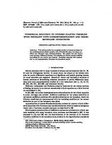
The numerical solution Iλ of the regularized system of normal equations (28), with λ = λopt given by eqn. (31), provides only a discrete distribution of the stream function at the global nodes of the BEM mesh employed. However, these discrete values should be extended to a continuous distribution of the numerical stream function over the entire coil surface Γcoil and this is achieved by employing the contours of the stream function using its discrete distribution and the Matlab (The Mathworks, Inc., Natick, MD, USA) contouring function. Hence, in the sequel, the numerically retrieved solutions of the inverse problem given by eqn. (8) are presented in terms of the contours of the stream function as described above. Figures 1(a) and (b) present the contours of the stream function in the θ − cos φ plane corresponding to the hemispherical x- and z-gradient coils, respectively, obtained using the optimal regularization parameter λopt given by eqn. (31), L = 351 internal points in the region of interest and N = 2840 linear, quadratic and cubic triangular boundary elements. It should be noted that, the so-called Lambert cylindrical equal-area projection, i.e. the θ − cos φ plane, has been used to represent the 2D contours of the stream function. From these figures it can be seen that, for the examples investigated in this study, the numerical results retrieved using linear boundary elements are more inaccurate than those obtained by employing higher-order boundary elements, with the mention that there are no major quantitative differences between the contours of the stream function corresponding to quadratic and cubic triangular elements.

0.5

0.5

0.4

0.4

0.3

0.3

0.2

0.2

0.1

0.1

0

1

2

3

θ

4

5

6

0

1

2

(a)

3

θ

4

5

6

(b)

Figure 1: The contours of the stream function corresponding to the hemispherical (a) x-, and (b) z-gradient coils, obtained using λ = λopt , L = 351 internal points in Ω and N = 2840 linear ( ), quadratic (− −) and cubic (· · · ) triangular boundary elements. WIT Transactions on Modelling and Simulation, Vol 44, © 2007 WIT Press www.witpress.com, ISSN 1743-355X (on-line)

Boundary Elements and Other Mesh Reduction Methods XXIX

331

0.9

0.9

0.8

0.8

0.7

0.7

0.6

0.6

cos φ

cos φ

The convergence of the proposed numerical method with respect to refining the BEM mesh size is illustrated in Figures 2(a) and (b) which present the contours of the stream function corresponding to the hemispherical x- and z-gradient coils, respectively, obtained using the optimal regularization parameter λopt chosen according to eqn. (31), L = 351 internal points in the region of interest and various numbers of quadratic triangular boundary elements (Ne = 6), namely N ∈ {1128, 1888, 2840}. Although an analytical solution for the contours of the stream function is not available, we can conclude from these figures that the Tikhonov regularization method described in Section 4, in conjunction with the divergence-free BEM presented in Section 3, is convergent with respect to increasing the number of boundary elements used to discretise the coil surface Γcoil . Furthermore, the finer the BEM mesh size is then the smoother contours of the stream function corresponding to the hemispherical x- and z-gradient coils.

0.5

0.5

0.4

0.4

0.3

0.3

0.2

0.2

0.1

0.1

0

1

2

3

θ

4

5

6

0

1

2

(a)

3

θ

4

5

6

(b)

Figure 2: The contours of the stream function corresponding to the hemispherical (a) x-, and (b) z-gradient coils, obtained using λ = λopt , L = 351 internal points in Ω and various numbers of quadratic triangular boundary elements, i.e. Ne = 6, namely N = 1128 ( ), N = 1888 (− −) and N = 2840 (· · · ).

6 Conclusions In this paper, we have investigated the design of hemispherical gradient coils for MRI by considering the reconstruction of a divergence-free surface current distribution from knowledge of the magnetic flux density in a prescribed region of interest. This inverse problem was formulated in the framework of static electromagnetism using its corresponding integral representation according to potential theory. In order to retrieve an accurate and physically correct numerical solution of this inverse problem, a minimisation problem for the Tikhonov functional was WIT Transactions on Modelling and Simulation, Vol 44, © 2007 WIT Press www.witpress.com, ISSN 1743-355X (on-line)

332 Boundary Elements and Other Mesh Reduction Methods XXIX solved, in conjunction with a novel higher-order BEM which satisfies the continuity equation for the current density. The numerical solutions were presented in terms of the contours of the stream function and using various types of boundary elements. For the examples analysed, it was proved the efficiency of the proposed method, as well as an improvement in the accuracy of the numerical solutions in the case of higher-order elements. However, there are no major quantitative differences between the contours of the stream function corresponding to quadratic and cubic triangular elements.

References [1] Turner, R. Gradient coil design: A review of methods. Magnetic Resonance Imaging, 11, pp. 903–920, 1993. [2] Leggett, J., Crosier, S., Blackband, S. & Bowtell, R.W. Multilayer transverse gradient coil design. Concepts in Magnetic Resonance B: Magnetic Resonance Engineering, 16, pp. 38–46, 2003. [3] Green, D., Leggett, J. & Bowtell, R.W. Hemispherical gradient coils for magnetic resonance imaging. Magnetic Resonance in Medicine, 54, pp. 656–668, 2005. [4] Jackson, J.D. Classical Electrodynamics, John Wiley & Sons: New York and London, 1962. [5] Brebbia, C.A., Telles, J.F.C. & Wrobel, L.C. Boundary Element Techniques, Springer-Verlag: Berlin and New York, 1984. [6] Tiknonov, A.N., & Arsenin, V.Y. Methods for Solving Ill-Posed Problems, Nauka: Moscow, 1986. [7] Hansen, P.C. Rank-Deficient and Discrete Ill-Posed Problems: Numerical Aspects of Inversion, SIAM: Philadelphia, 1998.

WIT Transactions on Modelling and Simulation, Vol 44, © 2007 WIT Press www.witpress.com, ISSN 1743-355X (on-line)