Numerical Solution of the Inverse Electrocardiography Problem with ...

ISSN 0278-6419, Moscow University Computational Mathematics and Cybernetics, 2008, Vol. 32, No. 2, pp. 61–68. © Allerton Press, Inc., 2008. Original Russian Text © A.M. Denisov, E.V. Zakharov, A.V. Kalinin, V.V. Kalinin, 2008, published in Vestnik Moskovskogo Universiteta. Vychislitel’naya Matematika i Kibernetika, 2008, No. 2, pp. 5–10.

Numerical Solution of the Inverse Electrocardiography Problem with the Use of the Tikhonov Regularization Method A. M. Denisova, E. V. Zakharova, A. V. Kalinina, and V. V. Kalininb a

Department of Mathematical Physics, Faculty of Computational Mathematics and Cybernetics, Moscow State University, Leninskie Gory, Moscow, 119992 Russia b Bakulev Center for Cardiovascular Surgery, Russian Academy of Sciences, Rublevskoe Shosse 135, Moscow, 121552 Russia e-mail: [email protected] Received September 4, 2007

Abstract—The inverse electrocardiography problem related to medical diagnostics is considered in terms of potentials. Within the framework of the quasi-stationary model of the electric field of the heart, the solution of the problem is reduced to the solution of the Cauchy problem for the Laplace equation in R3. A numerical algorithm based on the Tikhonov regularization method is proposed for the solution of this problem. The Cauchy problem for the Laplace equation is reduced to an operator equation of the first kind, which is solved via minimization of the Tikhonov functional with the regularization parameter chosen according to the discrepancy principle. In addition, an algorithm based on numerical solution of the corresponding Euler equation is proposed for minimization of the Tikhonov functional. The Euler equation is solved using an iteration method that involves solution of mixed boundary value problems for the Laplace equation. An individual mixed problem is solved by means of the method of boundary integral equations of the potential theory. In the study, the inverse electrocardiography problem is solved in region Ω close to the real geometry of the torso and heart. DOI: 10.3103/S0278641908020015

1. INVERSE ELECTROCARDIOGRAPHY PROBLEM The inverse electrocardiography problem is an important mathematical problem arising in medical diagnostics. This problem is known in several formulations. The inverse electrocardiography problem formulated in terms of potentials is considered to mean the problem of computational reconstruction of the potential of the electric field of the heart on its exterior (epicardial) surface from the registered potential on the surface of the chest [1, 2]. The inverse electrocardiography problem is topical, because information obtained from recorded surface electrocardiograms turns out to be insufficient for currently developed methods (including surgical methods) of treatment of cardiac-rhythm disturbances. The distribution of the potential of the electric field of the exterior (epicardial) or interior (endocardial) heart surface contains information necessary for new clinical methods. Within the framework of diagnostic techniques applied in modern medical practice, such information can be obtained only during surgical operations. The following biophysical model is used in the formulation of the inverse electrocardiography problem [3, 4]. The chest is considered as a conductor of the second kind with a constant conductivity coefficient. The conductor occupies a bounded spatial region and is embedded in air, i.e., in a dielectric medium. The electric field of the heart is described with the use of electrodynamic models of stationary currents, because the electric-field potential satisfies the Poisson equation. Sources of the electric field are located in the cardial-muscle tissue. In the spatial region bounded by the exterior heart surface and the body surface, there are no field sources and the field potential satisfies the Laplace equation. On the chest surface that contacts with air (the conductor/dielectric interface), the normal component of the electric-field intensity is zero. The measured potential of the electric field of the heart is known on this part of the chest surface. It is necessary to find the potential of the electric field on the exterior surface of the heart. Let us consider the mathematical formulation of this problem under the assumption that the chest surface is closed and the potential of the electric field of the heart is known on the entire chest surface and the normal derivative of the potential is zero. 61

62

DENISOV et al.

2. MATHEMATICAL FORMULATION OF THE PROBLEM Let Ω be a region in space R3. This region is bounded from outside and inside by closed surfaces S1 and S2, respectively. Surfaces S1 and S2 are assumed rather smooth. It is necessary to find function u(x, y, z) such that ∆u ( x, y, z ) = 0,

( x, y, z ) ∈ Ω

(1)

and u ( x, y, z ) = U ( x, y, z ), ∂u ------ ( x, y, z ) = 0, ∂n

( x, y, z ) ∈ S 1 ,

(2)

( x, y, z ) ∈ S 1 .

(3)

This problem is called the Cauchy problem for the Laplace equation. The Cauchy problem for the Laplace equation is a classic example of an ill-posed problem. A great number of studies are devoted to investigations of the uniqueness and conditional stability of its solution (see, e.g., [5] and the literature cited therein). Several regularizing algorithms based on various principles have been developed for numerical solution of the Cauchy problem [6–9]. In this study, on the basis of the Tikhonov regularization method [10], we develop a numerical algorithm for solution of Cauchy problem (1)–(3) for the Laplace equation in a 3D region. 3. TIKHONOV REGULARIZATION METHOD FOR SOLUTION OF THE INVERSE ELECTROCARDIOGRAPHY PROBLEM Consider the mixed boundary value problem ∆u ( x, y, z ) = 0,

( x, y, z ) ∈ Ω,

u ( x, y, z ) = v ( x, y, z ), ∂u ------ ( x, y, z ) = 0, ∂n

(4)

( x, y, z ) ∈ S 2 ,

(5)

( x, y, z ) ∈ S 1 .

(6)

Let u(x, y, z; v ) denote a solution to this problem for given function v (x, y, z), (x, y, z). ∈ S2. Problem (4)– (6) determines operator A that maps potential v on surface S2 into the potential on surface S1: Av ≡ u ( x, y, z; v ),

( x, y, z ) ∈ S 1 .

Then, problem (1)–(3) can be formulated as the problem of solution of the following operator equation of the first kind: Av = U ( x, y, z ),

( x, y, z ) ∈ S 1 .

(7)

We apply the Tikhonov regularization method [10] to solve this problem. Let exact solution v (x, y, z), (x, y, z) ∈ S2, to Eq. (7) exist for exact values U (x, y, z), (x, y, z) ∈ S1 but function U (x, y, z) be unknown. Approximation Uδ(x, y, z), (x, y, z) ∈ S1, is specified such that ||Uδ – U|| L2 ( S1 ) ≤ δ. It is necessary to construct approximate solution vδ(x, y, z) for known Uδ(x, y, z) and error δ. Consider the functional α

M [ v ] = Av – U δ

2 L2 ( S1 )

+α v

2 L2 ( S2 ) ,

α > 0.

(8)

Approximate solution vα is determined as an element that realizes the minimum of functional Mα[v ] where regularization parameter appropriately depends on the value of error δ; i.e., α = α(δ). Approximate solution vα can be found from the equation αv + A* Av = A*U δ ,

(9)

which is a necessary condition for the minimum of functional (8). Operator A* maps function g(x, y, z) that is specified on surface S1 into a function specified on surface S2. This operator is determined by the following mixed problem: MOSCOW UNIVERSITY COMPUTATIONAL MATHEMATICS AND CYBERNETICS

Vol. 32

No. 2

2008

NUMERICAL SOLUTION OF THE INVERSE ELECTROCARDIOGRAPHY PROBLEM

∆w ( x, y, z ) = 0, w ( x, y, z ) = 0,

63

( x, y, z ) ∈ Ω,

(10)

( x, y, z ) ∈ S 2 ,

(11)

∂w ------- ( x, y, z ) = g ( x, y, z ), ∂n

( x, y, z ) ∈ S 1 .

(12)

Denoting a solution to this problem for given function g as w(x, y, z; g), we obtain [11, 12] ∂w A*g = ------- ( x, y, z; g ), ∂n

( x, y, z ) ∈ S 2 .

Thus, operators A and A* entering Eq. (9) are determined by mixed problems (4)–(6) and (10)–(12), respectively. The value α = α(δ) of the regularization parameter can be found from the discrepancy principle [13]: Av α – U δ

L2 ( S1 )

= δ.

When certain preliminary information v˜ (x, y, z) on the form of the sought solution is known, the functional α M [ v ; v˜ ] = Av – U δ

2 L2 ( S1 )

+ α v – v˜

2 L2 ( S2 ) ,

α > 0,

can be introduced instead of functional (8). An approximate solution is found from the necessary condition α ( v – v˜ ) + A* Av = A*U δ

(13)

for the minimum. It follows from the foregoing that construction of an approximate solution is reduced to solution of Eq. (9) or (13). Now, let us consider methods and algorithms for numerical solution of these equations and boundary value problems (4)–(6) and (10)–(12). 4. METHOD OF BOUNDARY INTEGRAL EQUATIONS. As has been shown in the previous sections, the main computational procedures are reduced to solution of Euler equations (9) or (13), which necessitates solution of mixed boundary value problems (4)–(6) and (10)–(12). It is a common computational practice to apply the finite element method (discretization of an entire 3D region) and the method of boundary integral equations (see, e.g., [14, 15]) for numerical solution of problems of the aforementioned type. The method of boundary integral equations is a classic mathematical tool of theoretical investigation of the solvability of boundary value problems for elliptical equations [16]. This method involves reduction of boundary value problems to Fredholm boundary integral equations of the first and second kinds. The subsequent discretization of the boundary integral equations also enables one to obtain numerical solutions to boundary value problems. An advantage of this method over the finite element method is that it is unnecessary to discretize entire region Ω. Two approaches are usually applied to pass from boundary value problems to boundary integral equations. According to the first approach, a solution is sought in the form of the single- or double-layer potential. In the second approach, the unknown boundary conditions are determined as solutions to the integral equations that follow directly from the fundamental Green’s formula (the third Green’s formula). The second method is more suited for solution of boundary value problems (4)–(6) and (10)–(12). Consider region Ω (Fig.1) with sufficiently smooth boundary ∂Ω = S1 ∪ S2. Potential u in Ω (including the boundary) satisfies the Laplace equation. With allowance for the fundamental solution to the Laplace equation, a solution can be represented in the following integral form for the points of boundary ∂Ω: 2πu ( M ) =

∫

S1 ∪ S2

∂ ( 1/r )⎞ ⎛ q ( P ) 1--- – u ( P ) --------------ds ⎝ r ∂n P ⎠

MOSCOW UNIVERSITY COMPUTATIONAL MATHEMATICS AND CYBERNETICS

Vol. 32

No. 2

2008

64

DENISOV et al.

S1 Ω

S2

Fig. 1. Region Ω.

or 2πu ( M ) +

∫

S1 ∪ S2

∂ ( 1/r ) u ( P ) --------------- ds = ∂n P

∫

S1 ∪ S2

1 q ( P ) --- ds, r

(14)

where M, P ∈ ∂Ω, r is the Euclidean distance between points M and P, 1/r is the fundamental solution to the Laplace equation in R3, nP is the unit vector of the inward normal at point P, and q(P) = ∂u ( P )/∂n P . Let us split surface ∂Ω into boundary elements dsi: S = ds1 ∪ ds2 ∪ … ∪ dsn. We introduce a system of n linearly independent basis elements (characteristic functions) ϕ1, ϕ2, …, ϕn that are defined as follows: ⎧ ϕ i ( s ) = 1, ⎨ ⎩ ϕ i ( s ) = 0,

s ∈ ds i , s ∉ ds i .

The potential and its normal derivative are decomposed in the system of basis functions ϕi (step approximation): n

u(s) =

∑ α ϕ ( s ), i

i

i=1

(15)

n

q(s) =

∑ β ϕ ( s ), i

i

i=1

where αi is the value of u(s) and βi is the value of q(s) at the center of gravity of the ith boundary element. The substitution of (15) into (14) yields (16)

Hu = Gq, where the elements of matrices H and G are determined as MOSCOW UNIVERSITY COMPUTATIONAL MATHEMATICS AND CYBERNETICS

Vol. 32

No. 2

2008

NUMERICAL SOLUTION OF THE INVERSE ELECTROCARDIOGRAPHY PROBLEM

65

⎧ ( 1/r ij ) ⎪ ∂----------------- ds, i ≠ j, ⎪ ∂n P ⎪Sj h ij = ⎨ ⎪ ∂ ( 1/r ij ) ⎪ ------------------ ds + 2π, i = j, ⎪ ∂n P ⎩Sj

∫ ∫

g ij =

1

- ds. ∫ ---r Sj

ij

Boundary S is split into parts S1 and S2 (Fig. 1), and the boundary conditions are imposed on each part. Therefore, it is convenient to represent Eq. (16) in the form H 11 H 12 u 1

=

H 21 H 22 u 2

G 11 G 12 q 1

,

G 21 G 22 q 2

(17)

H = [ H kl ], G = [ G kl ],

where index k is the number of the surface with fixed point M and index l is the number of the surface with variable point P. Mixed boundary value problems (4)–(6) and (10)–(12) are combined with boundary conditions (U2, Q1). Thus, with allowance for known conditions, system (17) can be represented in the form H 11 H 12 u 1 H 21 H 22 U 2

=

G 11 G 12 Q 1

(18)

.

G 21 G 22 q 2

From representation (18), one can obtain explicit matrix equations for a solution to the mixed boundary value problem, i.e., for determination of u1 and q2. Since the mixed boundary value problem is an Hadamard well-posed problem, the matrices of these equations are well-conditioned and can easily be inverted. 5. SIMULATION RESULTS In this section, we present results of numerical solution of the inverse electrocardiography problem. The simulation is performed according to the following scheme: (i) Computation region Ω is specified, (ii) A system of electric-field sources is specified, (iii) The field of specified sources is calculated on surfaces S1 and S2 from the known relationships of the potential theory, (iv) A Gaussian noise of the intensity ranging from 1 to 15% is added to the potential on surface S1, (v) The inverse problem of calculation of the potential on surface S2 from noisy data is solved, (vi) The obtained solution is compared to a reference one. As the calculation region, we used the geometric configuration displayed in Fig. 1. Dipole and quadrupole sources, as well as unit positive and negative charges randomly distributed in space, were specified inside surface S2. The system of charges was formed such that the configuration of the electric field on surface S2 simulated the electric field of the heart. The surface was triangulated according the algorithms proposed in study [17]. The number of boundary elements (triangles) of the discretized surface was about 600– 1500. Next, the iteration method was applied to solve Eqs. (9) and (13). At each iteration step, direct mixed boundary value problems (4)–(6) and (10)–(12) were solved with the use of the method of boundary integral MOSCOW UNIVERSITY COMPUTATIONAL MATHEMATICS AND CYBERNETICS

Vol. 32

No. 2

2008

66

DENISOV et al. (a) 1.2 1.0 0.8 0.6 0.4 0.2 0 –0.2 –0.4 –0.6 –0.8 50

0

–50 (b)

0

50

0.8 0.6 0.4 0.2 0 –0.2 –0.4 –0.6 50

50 0

–50

0

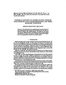
Fig. 2. Configuration of three spatially distributed field sources: (a) given configuration and (b) reconstructed configuration.

equations and the values of operators A and A* were calculated. The regularization parameter α was selected according to the discrepancy principle. For all the considered configurations of specified sources, the method exhibited stable convergence to the solution with an error of 2–15% at a noise intensity of 1%. Within the employed model sources, the solution accuracy did not depend on the character of the potential to be reconstructed (with allowance for the limitations imposed by the boundary-element method on the proximity of sources to the boundary). The quality of the solution can be estimated from Figs. 2 and 3. These figures show the distribution u = f(x, y) of the field potential in the upper part of the interior ellipsoid (see surface S2 in Fig. 1); x and y belong to the upper part of S2. MOSCOW UNIVERSITY COMPUTATIONAL MATHEMATICS AND CYBERNETICS

Vol. 32

No. 2

2008

NUMERICAL SOLUTION OF THE INVERSE ELECTROCARDIOGRAPHY PROBLEM

67

(a) 5 4 3 2 1 0 –1 –50 0 –40

–20 (b)

0

20

40

20

40

4.0 3.5 3.0 2.5 2.0 1.5 1.0 0.5 0 –0.5 –1.0 –50 0 –40

–20

0

Fig. 3. Configuration of three sources grouped on the upper part of the interior surface: (a) given configuration and (b) reconstructed configuration.

A system of three charges is presented in Fig. 2. The positive charge is in the upper part of the interior ellipsoid, and the two negative charges are situated symmetrically with respect to the ellipsoid’s center near the side boundaries. Figure 3 shows a system of three positive charges grouped in the upper part of the interior ellipsoid. Thus, the method proposed in this study enables one to solve the inverse electrocardiography problem for region Ω that is close to the real geometry of the torso and heart. The distribution of the electric-field potential on interior surface S2 adequately simulates the potential of the electric field of the heart. MOSCOW UNIVERSITY COMPUTATIONAL MATHEMATICS AND CYBERNETICS

Vol. 32

No. 2

2008

68

DENISOV et al.

ACKNOWLEDGMENTS This work was supported by the Russian Foundation for Basic Research, project no. 08-01-00314. REFERENCES 1. R. C. Barr and M. S. Spach, “Inverse Solutions Directly in Terms of Potentials,” in The Theoretical Basis of Electrocardiology, Ed. by C. V. Nelson and D. B. Geselowitz (Oxford Univ., London, 1976; Meditsina, Moscow, 1979), 294–304. 2. L. A. Bokeriya, V. V. Shakin, G. V. Mirskii, and I. P. Polyakova, Numerical methods of Electrophysiological Assessment of the Heart State (Vychisl. Tsentr Akad. Nauk SSSR, Moscow, 1987) [in Russian]. 3. MacLeod R.S., Brooks D.H. “Recent Progress in Inverse Problems in Electocardiology,” IEEE Eng. Med. Biol. Mag. 17 (1), 73–83 (1998). 4. C. Ramanathan, R. N. Ghanem, P. Jia, et al., “Noninvasive Electrocardiographic Imaging for Cardiac Electrophysiology and Arrhythmia,” Nature Medicine, 10, 422–428 (2004). 5. M. M. Lavrent’ev, V. G. Romanov, and S. P. Shishatskii, Ill-Posed Problems of Mathematical Physics (Nauka, Moscow, 1980; American Mathematical Society, Providence, R.I., 1986). 6. R. Lattes and J.-L. Lions, The Method of Quasi-Reversibility; Applications to Partial Differential Equations (American Elsevier, New York, 1969; Mir, Moscow, 1970). 7. V. A. Kozlov, V. A. Maz’ya, and A. V. Fomin, “On One Iterative Method of Solution of the Cauchy Problem for Elliptic Equations,” Zh. Vychisl. Mat. Mat. Fiz., 31 (1), 64–74 (1991). 8. V. B. Glasko, Inverse Problems of Mathematical Physics (Mosk. Gos. Univ., Moscow, 1984) [in Russian]. 9. P. N. Vabishchevich, V. B. Glasko, and Yu. A. Kriksin, “On Solution of One Hadamard Problem with the Use of a Tikhonov-Regularization Algorithm,” Zh. Vychisl. Mat. Mat. Fiz. 19 (6), 1462–1473 (1979). 10. A. N. Tikhonov and V. Ya. Arsenin, Solutions of Ill-Posed Problems (Nauka, Moscow, 1979; Halsted, New York, 1977). 11. S. I. Kabanikhin and A. L. Karchevsky, “Optimizational Method for Solving the Cauchy Problem for an Elliptic Equation,” J. Inverse Ill-Posed Problems, 3, 21–46, (1995). 12. Dihn Nho Hao and D. Lesnic, “The Cauchy Problem for Laplace’s Equation Via the Conjugate Gradient Method,” IMA J. Appl. Math. 65, 199–217 (2000). 13. V. A. Morozov, “Onthe Discrepancy Principle Involved in Solution of Operator Equations with the Use of the Regularization Method,” Zh. Vychislit. Matem. Matem. Fiz., 8 (2), 295–309 (1968). 14. C. A. Brebbia, J. C. F. Telles, and L. C. Wrobel, Boundary Element Techniques: Theory and Appiications in Engineering (Springer-Verlag, Berlin, 1984; Mir, Moscow, 1987). 15. C. Pozrikidis, A Practical Guide to Boundary Elements Methods with the Software Library BEMLIB (Chapman and Hall/CRC, London, 2002). 16. A. N. Tikhonov and A. A. Samarskii, Equations of Mathematical Physics (Nauka, Moscow, 2004; Pergamon, Oxford, 1964). 17. E. R. Gol’nik, A. A. Vdovichenko, and A. A. Uspekhov, “Construction and Application of a Preprocessor of Generation, Quality Control, and Optimization of Triangulation Grids of Contact Systems,” in Information Technologies (Voronezh. Gos. Techn. Univ., Voronezh, 2004), No. 4, pp. 2–10.

MOSCOW UNIVERSITY COMPUTATIONAL MATHEMATICS AND CYBERNETICS

Vol. 32

No. 2

2008