An investigation into the use of maximum likelihood ... - CiteSeerX

An investigation into the use of maximum likelihood classifiers, decision trees, neural networks and conditional probabilistic networks for mapping and predicting salinity

Fiona Evans School of Computing, Curtin University of Technology, GPO Box U1987, Perth, 6845, Western Australia. email: [email protected]

March 1998

presented as part of the requirements for the award of the Degree of Master of Science in Computer Science at the Curtin University of Technology

Acknowledgments The author gratefully acknowledges the support and advice given by my supervisors Dr. Geoff West and Dr Mark Gahegan. Thank you for your regular suggestions and timely feedback. Grateful acknowledgment also to the researchers of the Remote Sensing and Monitoring project of CSIRO Mathematical and Information Sciences. In particular, to Dr Norm Campbell for encouraging me to begin this thesis and providing support throughout its completion, to Ms Suzanne Furby for assistance with image processing and maximum likelihood classification and to Dr Harri Kiiveri for assistance with the design of the conditional probabilistic network. I would like to thank Agriculture WA hydrologists Doctors Don McFarlane, Ruhi Ferdowsian and Richard George for their assistance in providing ground data and aerial photograph interpretations. In addition, Mr John Sprigg from the Lower Slab Hut catchment and Mr Bill Ladyman from the Ryan’s Brook catchment for providing catchment-wide farm plans and enthusiastically awaiting the results of this research. Lastly, my thanks go to Ms Gillian Carter for reading the thesis and offering succinct suggestions about improvements to its readability. This research has included components from the project “Monitoring land condition in the upper Blackwood and Frankland-Gordon catchments” which was funded by the Land and Water Resources Research and Development Corporation.

II

Abstract This thesis investigates the use of different classifiers for integrating remotely sensed data with other spatial data derived from digital elevation models to produce maps showing areas affected by salinity in the south west agricultural region of Western Australia. A method is developed for accurately mapping and monitoring salinity on a broad-scale using costeffective data. In addition, a cost-effective method is presented for predicting areas at risk from salinity over broads regions. Maximum likelihood classification using single-date Landsat Thematic Mapper image is used as a benchmark to determine whether the integration of multi-temporal Landsat data and landform data produces more accurate salinity maps. Decision trees and neural networks are used to map saline areas in the Ryan’s Brook catchment, located approximately 50 kilometres southwest of Kojonup, using two Landsat images and two landform attributes (water accumulation and downhill slope). A conditional probabilistic network is then used to impose a known relationship between input attributes and salinity status. In this way, changes in salinity through time can be modelled using all of the available Landsat data. The results show a large improvement on the maximum likelihood, decision tree and neural network classifiers. The network is used to produce a time-series of salinity maps for the upper Blackwood and Frankland-Gordon catchments. These maps are used as inputs to the predictions of salinity risk areas. The prediction of salinity risk areas is approached using decision tree classifiers, so that the derived models can be easily interpreted by end-users. A simple decision tree for predicting salinity risk is developed. Rules are extracted from the decision tree, and refined to form some straightforward methods for assessing salinity risk on the ground.

III

Table of Contents Acknowledgments...................................................................................................... II Abstract ...................................................................................................................... III Table of Contents .....................................................................................................IV Table of Figures.......................................................................................................VII Table of Tables .........................................................................................................IX 1

2

3

Introduction ......................................................................................................... 1 1.1

Objectives........................................................................................................ 4

1.2

Implementation................................................................................................. 5

1.3

Evaluation ........................................................................................................ 6

1.4

Limitations and delimitations .............................................................................. 6

1.5

Thesis structure................................................................................................ 7

The study area and data preparation............................................................... 9 2.1

Introduction ...................................................................................................... 9

2.2

The study area.................................................................................................. 9

2.3

Ground truth data.............................................................................................10

2.4

Landsat TM pre-processing...............................................................................11

2.5

Digital elevation data........................................................................................12

2.6

Water accumulation .........................................................................................12

2.7

Drainage slope.................................................................................................14

2.8

Discussion ......................................................................................................14

Classification and accuracy assessment....................................................... 15 3.1

Introduction .....................................................................................................15

3.2

Classification...................................................................................................15

3.3

Criteria for selecting a classifier ........................................................................15

3.4

Resubstitution and cross validation ...................................................................16

3.5

Assessing accuracy.........................................................................................17

3.5.1

Overall accuracy...........................................................................................................................17

3.5.2

The Kappa statistic ......................................................................................................................18

3.5.3

Other methods for assessing accuracy ..................................................................................19

3.6

4

Discussion ......................................................................................................19

Maximum likelihood classification.................................................................. 20 4.1

Introduction .....................................................................................................20

4.2

Maximum likelihood classification......................................................................20

IV

4.2.1

Bayes’ theorem and maximum likelihood classification .....................................................21

4.2.2

Canonical variate analysis .........................................................................................................23

4.2.3

Neighbour-modified maximum likelihood classification .....................................................24

4.3 4.3.1

Selection of training sites ...........................................................................................................25

4.3.2

Canonical variate analyses........................................................................................................25

4.3.3

Classification accuracies ...........................................................................................................28

4.3.4

Neighbourhood-modified classification ..................................................................................30

4.4

5

5.1

Introduction .....................................................................................................34

5.2

Decision tree classification ...............................................................................35

5.2.1

Criteria for evaluating splits .......................................................................................................37

5.2.2

Tests on continuous attributes ..................................................................................................38

5.2.3

Tests on linear combinations of continuous attributes ........................................................39

5.2.4

Pruning...........................................................................................................................................39

Mapping salinity using decision trees .................................................................40

5.3.1

Attribute selection.........................................................................................................................40

5.3.2

Decision tree accuracies for mapping salinity.......................................................................42

5.4

Discussion ......................................................................................................46

Neural networks................................................................................................ 49 6.1

Introduction .....................................................................................................49

6.2

Neural network classification.............................................................................50

6.2.1

Neural networks with a single layer of weights ......................................................................50

6.2.2

Logistic discrimination................................................................................................................52

6.2.3

Two-layer perceptrons ................................................................................................................53

6.2.4

Training the network: error back-propagation ........................................................................54

6.2.5

Determining the structure and initialising the weights .........................................................55

6.3

Mapping salinity using neural networks...............................................................56

6.3.1

Mapping salinity using multi-layer perceptrons .....................................................................57

6.3.2

Modification of the training data.................................................................................................61

6.4

7

Discussion ......................................................................................................32

Decision trees................................................................................................... 34

5.3

6

Maximum likelihood classification of the Landsat data.........................................25

Discussion ......................................................................................................63

Conditional probabilistic networks ................................................................ 66 7.1

Introduction .....................................................................................................66

7.2

Classification using conditional probabilistic networks.........................................67

7.2.1

Neighbourhood modifications to CPNs ..................................................................................68

7.3

Salinity change maps using CPNs .....................................................................69

7.4

Discussion ......................................................................................................72

V

8

Salinity prediction............................................................................................. 74 8.1

Introduction .....................................................................................................74

8.2

Predicting salinity using a decision tree classifier................................................74

8.2.1

Attribute selection.........................................................................................................................75

8.2.2

Decision trees for predicting salinity risk ................................................................................76

8.3 8.3.1

Maximal pruning...........................................................................................................................78

8.3.2

Simple rules for predicting salinity risk....................................................................................80

8.4

9

A simple decision tree model of salinity risk .......................................................78

Discussion ......................................................................................................81

Conclusions and further work ........................................................................ 82 9.1

Conclusions ....................................................................................................82

9.1.1

Mapping salinity............................................................................................................................82

9.1.2

Predicting salinity risk areas......................................................................................................85

9.2

Further work ....................................................................................................86

9.2.1

Neighbourhood modifications to decision trees ...................................................................86

9.2.2

Pre-processing neural network inputs ....................................................................................87

9.2.3

Using decision trees to aid the design of neural networks .................................................88

9.2.4

Ensembles of classifiers ...........................................................................................................88

9.2.5

Learning conditional probability distributions ........................................................................89

9.2.6

Improving accuracy with additional data sets.........................................................................89

9.2.7

Predicting salinity using conditional probabilistic networks ................................................90

10 Bibliography ...................................................................................................... 91 Appendix A: Example farm plan.............................................................................. 99

VI

Table of Figures Figure 1 The Blackwood and Frankland-Gordon catchments. .............................................10 Figure 2 Calibrated (i) 1989 and (ii)1990 Landsat images with bands 4, 5, 7 in R, G, B.........12 Figure 3 (i) water accumulation and (ii) downhill slope maps - increasing values are shown from black to white. ..........................................................................................14 Figure 4 Fitted Gaussian distributions..............................................................................22 Figure 5 Canonical variate plot for August 1989.................................................................26 Figure 6 Canonical variate plot for September 1990. ..........................................................27 Figure 7 Canonical variate plot for September 1993. ..........................................................27 Figure 8 Canonical variate plot for August 1994................................................................28 Figure 9 (i) 1989 and (ii) 1990 Landsat classifications........................................................29 Figure 10 Neighbourhood-modified classifications for (i) 1989 and (ii) 1990. .........................31 Figure 11 The decision tree structure. ..............................................................................35 Figure 12 Given axes that show the attribute values and colours corresponding to class labels (i) axis-parallel and (ii) oblique decision boundaries..............................................36 Figure 13 Salinity map produced using c4.5. ....................................................................45 Figure 14 Salinity map produced using oc1. .....................................................................46 Figure 15 Representation of a linear function as a one-layer network - each line corresponds to a network weight. .............................................................................................51 Figure 16 A network with one layer of weights. .................................................................52 Figure 17 A network with two layers of weights.................................................................54 Figure 18 Kappa value calculated over the validation data plotted against number of training iterations for an MLP with one hidden unit and with random initialisation. ...............57

VII

Figure 19 Kappa value calculated over the validation data plotted against number of training iterations for an MLP with one hidden unit, initialised using pairwise discriminant functions..........................................................................................................58 Figure 20 Kappa value calculated over the validation data plotted against number of training iterations an MLP with four hidden units and random initialisation.........................58 Figure 21 Salinity map produced using a two-layer network with 10 hidden layer units..........61 Figure 22 A simple CPN for mapping salinity....................................................................68 Figure 23 A simple CPN with neighbourhood effects included.............................................69 Figure 24 The CPN used for mapping salinity. ..................................................................70 Figure 25 Salinity maps produced using the conditional probabilistic network. .....................71 Figure 26 Predicted risk maps produced using various options of c4.5. ...............................77 Figure 27 Predicted salinity risk areas produced using a maximally pruned tree. .................78 Figure 28 A simple decision tree for predicting salinity risk. ...............................................79

VIII

Table of Tables Table 1 1989 classification statistics. ..............................................................................29 Table 2 1990 classification statistics. ..............................................................................29 Table 3 1993 classification statistics. ..............................................................................30 Table 4 1994 classification statistics. ..............................................................................30 Table 5 1989 neighbourhood-modified classification statistics. ...........................................31 Table 6 1990 neighbourhood-modified classification statistics. ...........................................31 Table 7 1993 neighbourhood-modified classification statistics. ...........................................31 Table 8 1994 neighbourhood-modified classification statistics. ...........................................31 Table 9 C4.5 accuracies and Kappa values averaged over 5 partitions.................................41 Table 10 Oc1 (axis-parallel) accuracies and Kappa values averaged over 5 partitions............42 Table 11 Oc1 (oblique) accuracies and Kappa values averaged over 5 partitions...................42 Table 12 C4.5 accuracies and Kappa values averaged over 5 partitions. ..............................43 Table 13 Kappa values for each cross-validation partition. .................................................43 Table 14 Oc1 accuracies and Kappa values averaged over 5 partitions................................45 Table 15 Neural network accuracies and Kappa values averaged over 5 partitions. ...............59 Table 16 Neural network accuracies and Kappa values averaged over 5 partitions. ...............59 Table 17 Neural network accuracies for each partition. ......................................................60 Table 18 Neural network accuracies and Kappa values averaged over 5 partitions. ...............62 Table 19 C4.5 accuracies and Kappa values using 3 classes.............................................62 Table 20 Broomehill CPN accuracies and Kappa values. ...................................................71 Table 21 Ryan's Brook CPN accuracies and Kappa values. ...............................................71 Table 22 Accuracies and Kappa values for salinity risk prediction. ......................................76

IX

Table 23 Salinity risk prediction accuracies and Kappa values. ..........................................76

X

1

Introduction

Salinisation of streams and extension of the area of salt-affected soils is perhaps one of the most wide-spread and significant effects of clearing land for agriculture in southern Australia generally. Among the most seriously affected agricultural areas are those inland of the Darling Range in Western Australia, and the drier northern areas of Victoria.

M. J. Mulcahy (1978)

Seventy percent of Australia’s dryland salinity is in Western Australia. It is estimated that 1.8 million hectares, or approximately 10%, of Western Australian land cleared for agriculture is affected by salinity, causing agricultural production losses of $64 million a year (Ferdowsian et al., 1996; State Salinity Action Plan, 1996). The WA government has recognised the need for a coherent plan to reduce the extent of salinity and its effects on the state. The 1996 Salinity Action Plan stresses the requirement for accurate monitoring of salt-affected land, and pledges $200 000 pa to establish a regular program of satellite image evaluation using the Landsat Thematic Mapper (TM) satellite. The plan aims to provide the most reliable and consistent recording of the area of salt-affected land, remnant vegetation extent and establishment of deep-rooted perennials throughout the agricultural areas of southwest WA. Landsat satellite images provide a means for mapping land status and condition over broad areas. The images are routinely archived on acquisition, and are inexpensive for broad-scale monitoring. Maximum likelihood procedures have traditionally been used as a baseline for the classification of remotely sensed data. For instance, Apan (1997) uses maximum likelihood classification to assess the utility of Landsat data for mapping forest rehabilitation and Basham May et al. (1997) use maximum likelihood classification to compare the effectiveness of Landsat and SPOT data for vegetation classification. Studies conducted by the CSIRO Mathematical and Information Sciences (CMIS) have shown that data from the Landsat satellite can be used to map areas affected by salinity (Wheaton et al., 1992; 1994) using maximum likelihood classification. This thesis proposes that the accuracy with which salinity can be mapped using Landsat data could be improved by using multi-temporal Landsat data, and by incorporating topographical

1

information into the classification procedures. Topography is an important determinant of ground water flow and surface flow, and of the location of discharge areas where ground water rises to the surface (Salama et al., 1991). Increased discharge causes salinity to form in valley floors and depressions (Salama et al., 1993). Salama et al. (1991) establish basin slope to be the most important factor for understanding groundwater flow. The impacts of landform (eg. hilltop, slope, valley floor) and basin slope on salinisation suggest that the accuracy of salinity can be improved with the use of additional data describing these factors. This hypothesis is supported by the results of study by Furby et al. (1995). They used data derived from digital elevation models (DEMs) to improve the accuracy of salinity mapping using Landsat data. Since it is harder to assume known class distributions, maximum likelihood procedures are less suited to integrating multi-temporal Landsat data with other spatial data sets such as landform type or slope. This thesis proposes that non-parametric decision tree and neural network classifiers are more suitable for mapping salinity using Landsat data from several dates and attribute data that relate to landform. The advantages of using decision tree classifiers and neural networks are that: 1. They enable relationships between the Landsat data and terrain data to be extracted without prior knowledge about the ways in which these data interact. 2. They provide a means to automatically partition the attribute space into subregions corresponding to subclasses of the broader classes of interest. These advantages are particularly relevant to this application, because ground truth data for mapping salinity do not contain information about specific cover types. Ground data are usually provided in the form of farm-plans, which delineate salt-affected areas, remnant vegetation and paddock boundaries, or as interpretations of aerial photographs, which delineate only those areas which are salt-affected and those which are not (see Appendix A). The farm-plans and interpretations can only be used to select training areas that are labelled as either salt or not salt. However, the classes salt and not salt are comprised of many spectrally different subclasses corresponding to different land cover types. For instance, these may be evident as bare scalded areas, salt-affected areas re-vegetated with salttolerant species, salt-affected land with salt-tolerant native species or marginally affected ares within pasture paddocks that can be recognised by a cover of barley-grass. Land that is 2

not salt-affected includes remnant vegetation (woodland, heath, forest, scrubland and mallee), crops (wheat, barley, oats, lupins, canola), pastures, bare paddocks, lakes and rivers, and urban areas. A disadvantage of maximum likelihood classification arises from the time and effort required to prepare the training samples. Since, maximum likelihood procedures require training data for each spectral class in the image, mapping salt-affected land from Landsat imagery using maximum likelihood can be very time-consuming. The ground data are used as a guide to interpret the image and select sites that include each of the (spectral) subclasses mentioned above. Using multiple images requires that the training sites must be examined in each of the images, because the ground cover may have changed between the two dates. For instance, a cropped paddock in one year might be used for pasture in the following year. If landform attributes are also included, then training areas must be extended to include all possible combinations of ground cover in each year and landform class. Decision tree classifiers and neural networks can be used to overcome this disadvantage. They can save time and resources by automatically identifying the subclasses within the broader salt and not salt classes. Decision tree classifiers divide the attribute space into homogeneous regions within which each point has the same class. Each leaf of the decision tree corresponds to a region in the attribute space (or subclass) which is allocated a class label of salt or not salt. Multilayer perceptrons (MLPs), a form of neural network classifier, define a number of hyperplanes which divide the attribute space into homogeneous regions within which each point has the same class. Each node in the hidden layer of the MLP corresponds to a particular hyperplane. Given the number of hyperplanes required to subdivide the attribute space into a sufficient number of regions, then the regions defined by the hyperplanes of an MLP will correspond to the subclasses of salt and not salt. One disadvantage of decision tree and neural network classifiers for mapping salinity; however, it is difficult to incorporate prior knowledge about the relationships between attributes, and their relationship with salinity. Conditional probabilistic networks (or expert systems) provide a framework for including prior knowledge in the classification model. Since saline areas are unlikely to become smaller as time progresses and there is a relationship between the presence of salinity for different dates, this framework is particularly useful

3

when considering a time series of Landsat images. The conditional probabilistic network approach enables these relationships to be included in the classification process. This thesis investigates possible improvements in salinity mapping that can be gained using this technique. Predicting areas at risk from future salinity is also important for land management, since it allows resources to be allocated to the prevention of further loss of arable land. Making predictions is very difficult. At present, reliable predictions can only be made using smallscale data-intensive process-based models, or by hydrologists with extensive experience and local knowledge. This thesis develops a simple decision tree for predicting salinity risk using ground truth data provided by several experienced hydrologists. The decision tree model can be used to predict salinity risk areas over broad areas using cost-effective data and minimal human input, thus providing potentially significant financial savings over current methods for risk prediction. This thesis aims to produce methodologies that provide answers to two important questions about salinity: 1. Can the areas of land affected by salinity be accurately mapped and monitored on a broad scale, using cost-effective satellite imagery and landform data? 2. Can the same data be used to predict areas at risk from salinity in the future using a simple model that provides information about causes of salinity? These questions are answered by contrasting traditional methods for the classification of remotely sensed data with newer classification techniques; specifically decision trees, neural networks and conditional probabilistic networks. 1.1

Objectives

Objective 1 To determine whether the accuracy of salinity mapping using Landsat data can be improved by integrating multi-temporal sequences of images with landform data, and to develop a method for accurately mapping salinity on a broad scale using cost-effective Landsat and landform data. Sub-objective 1.1 4

To investigate the use of maximum likelihood classifiers for mapping salinity using a single Landsat image. Sub-objective 1.2 To investigate the use of decision tree classifiers for integrating two successive dates of Landsat imagery with landform data to map salinity. Sub-objective 1.3 To investigate the use of neural networks for integrating two successive dates of Landsat imagery with landform data to map salinity. Sub-objective 1.4 To investigate the use of conditional probabilistic networks for including prior knowledge about the relationships between input attributes and their relationship with salinity. Objective 2 To develop a cost-effective method for predicting areas at risk from salinity using a simple model that can be interpreted to help understand the process of salinisation. 1.2

Implementation

Image processing is implemented using ERMapper. Data integration methods are implemented within the GRASS geographical information system. Interfaces with GRASS have been used to transfer data between ERMapper, GRASS and the classification software that has been used. The author wrote code for all such interfaces. The statistical software package Splus has been used to calculate accuracy statistics. Unix scripts and Splus programs have been written for extracting accuracies from classification software outputs (unformatted text) and calculating accuracy statistics and averages. In order that the experiments described here may be evaluated and repeated by other scientists, the Ryan’s Brook and Broomehill data are available from the web page http://www.cmis.csiro.au/rsm/people/fionae/MSc/.

5

1.3

Evaluation

This thesis will meet its objectives by: 1. Developing procedures with which multi-temporal Landsat imagery and landform attributes can be used to map salinity using decision trees, neural networks and conditional probabilistic networks, and comparing the resulting accuracies and maps with those achieved using maximum likelihood classification of single-date images. 2. Producing an operational procedure for predicting salinity risk areas over broadscales using cost-effective Landsat and landform data. 1.4

Limitations and delimitations

This thesis performs a thorough investigation into the use of maximum likelihood classification, decision trees, neural networks and conditional probabilistic networks for mapping and predicting salinity. However, it presents no new algorithms for any of the classification procedures. The input data are provided to the classifiers without any preprocessing or scaling. Transformations of the input attribute data are avoided in order that interpretations of the prediction model might be made. The investigations performed are strictly application specific; gains in accuracy may not be generalisable to other applications using similar methods. In addition, the investigations are locationally specific; methods for mapping and predicting salinity may not provide similar accuracies if applied outside of the WA wheatbelt. The research is limited by the form of ground data that is used. Since the thesis aims to develop a cost-effective method for mapping salinity, ground data have been provided in simple, easily attainable forms. The ground data were provided as air-photo interpretations and farm-plans that delineated salt-affected areas and non-affected areas (see section 2.3). The data were then digitised into two broad classes: salt and not salt. The performance of the classifiers investigated is limited by the 2-class training data; likely improvements could be gained by subdividing the training data into more classes. This is not investigated due to the difficulty and associated costs of obtaining more detailed ground data.

6

1.5

Thesis structure

The structure of this thesis departs from tradition. In an effort to improve readability, a literature review comprised of background material is included in each of the relevant chapters. The contents of the thesis are outlined below. Chapter 2 describes the study area and sub-areas for which ground data are available. The input attribute data are described, along with the pre-processing required for multi-temporal analysis. The development of attributes that act as surrogates for landform (ie. water accumulation and downhill slope) is described. Chapter 3 defines the classification problem and discusses methods for assessing the accuracy of a classifier. The emphasis of the chapter is on the methods used in the thesis. Chapter 4 investigates the use of maximum likelihood classification to produce salinity maps for four dates, using a single Landsat image in each case. The theory behind maximum likelihood classification and neighbourhood-modified maximum likelihood classification is described in section 4.2. The methods of Wheaton et al. (1994) are applied, and the maximum likelihood classifier is then modified so that information from neighbouring pixels can be used to update the class label for each pixel. The results form a baseline with which the results achieved using other classifiers are compared. Chapter 5 investigates the application of decision trees to mapping salinity using multitemporal Landsat data and landform data derived from digital elevation models. The theory behind decision tree classification is described in section 5.2, with particular reference to the implemented algorithms. The accuracy with which salinity mapping can be performed using decision tree classifiers is assessed, and the results are compared with those achieved using maximum likelihood techniques. Chapter 6 examines the application of neural networks (MLPs in particular) to mapping salinity, again using multi-temporal Landsat data and landform data derived from digital elevation models. Required background material is presented in section 6.2. The accuracy with which salinity mapping can be performed using neural network classifiers is assessed, and the results are compared with those achieved using both decision tree and maximum likelihood techniques. The efficacy of using MLPs to sub-divide the attribute space into

7

regions that correspond to subclasses of salt and not salt is examined. Consequently, chapter 6 investigates the use of MLPs as exploratory data tools with respect to mapping salinity. Chapter 7 investigates the use of a conditional probabilistic network for producing maps of salinity that are consistent through time. Some brief explanation of the theory behind CPNs is presented in section 7.2. The landcover classifications produced using neighbourhoodmodified maximum likelihood techniques (chapter 4) and landform type are used as inputs to the network. Conditional probabilities are initialised using the error estimates from the maximum likelihood classifications and prior knowledge about joint relationships between the input attributes and salinity. The probabilities are refined in an iterative procedure. The results are favourably compared with those achieved using maximum likelihood classifiers, decision trees and neural networks. Chapter 8 of the thesis investigates the use of decision tree classifiers for predicting salinity risk areas from a time-series of salinity maps and DEM-derived landform data. The decision tree classifier is selected over other methods because it provides a means for exploratory data analysis and an understanding of the relationships between the input attributes and salinity risk. In addition, the c4.5 classifier is used to derive rules for predicting salinity risk. This chapter addresses the second objective of the thesis, which aims to develop a costeffective method for predicting areas at risk from salinity using a simple model that can be interpreted to help understand the process of salinisation. A discussion of the results of the thesis and suggestions for future work are presented in chapter 9.

8

2

The study area and data preparation

2.1

Introduction

This thesis aims to develop cost-effective methods for accurately mapping and predicting salinity over broad scales. It has been previously shown that Landsat data can provide a costeffective tool for mapping salinity (Wheaton et al., 1992; 1994). By investigating whether the integration of multi-temporal data with landform information can improve the accuracy with which salinity can be mapped, the work presented in this thesis aims to expand upon previous work in mapping salinity using Landsat data. This chapter describes the study area and sub-areas that are used to evaluate the classifiers investigated in the thesis. The ground data are described in section 2.3. Section 2.4 describes the pre-processing undertaken to prepare the Landsat data for multi-temporal analysis and image classification. This thesis proposes that information about landform can be used to improve the accuracy of salinity mapping. This requires the derivation of attributes that can act as surrogates for landform from readily available and cost-effective data sources. Digital contour data are readily (and cheaply) available for the Western Australian wheatbelt and can be processed to form gridded digital elevation models (DEMs). The procedure for producing gridded DEMs is described in section 2.5. Sections 2.6 and 2.7 describe the derivation of two landform attributes, water accumulation and downhill slope, which act as surrogates for landform and are easily derived from DEMs. 2.2

The study area

A rectangular study area containing the upper Blackwood and Frankland-Gordon catchments was selected. The study area is shown in Figure 1. The area covered by the Landsat data is shaded grey, and the Ryan’s Brook, Broomehill and Date Creek study areas are highlighted.

9

Figure 1 The Blackwood and Frankland-Gordon catchments.

2.3

Ground truth data

Individual farmers and catchment groups throughout the Blackwood and Frankland-Gordon catchments provided ground truth. Data were provided in the form of farm-plans, areas marked on maps and image interpretations. An example farm plan is attached in Appendix A. So that maximum likelihood techniques could be evaluated, the ground truth sites were examined in each of the Landsat images to determine the ground cover for each date. The Ryan’s Brook catchment, fully located within the Frankland-Gordon catchment, is used as a testbed for the comparison of decision tree and neural network classifiers because farm plans exist for the entire catchment. The plans, provided by the local catchment group, show areas affected by salinity and waterlogging. These data are also used as independent validation sites for the maximum likelihood classifications. The ground truth data for the Ryan’s Brook catchment are comprised of 98 non-saline sites and 47 saline sites. The non-

10

saline sites covered 4400 pixels and the saline sites covered 1195 pixels. These sites were digitised using the farm plans as a guide. Ground data for salinity prediction were available in three areas: 1. The upper Kent River catchment, located south of the Frankland-Gordon. 2. The Broomehill study area, located on the catchment boundary between the Blackwood and Frankland-Gordon catchments. 3. The Date Creek subcatchment, fully located in the Upper Blackwood catchment. The data were provided in the form of stereoscopic aerial photograph interpretations by Agriculture Western Australia ∗ hydrologists Dr Ruhi Ferdowsian and Dr Richard George. Both saline areas and areas predicted to be at risk from salinity were marked as overlays on the air-photos. These were digitised and rectified to AMG coordinates. 2.4

Landsat TM pre-processing

Landsat data were acquired for the Blackwood and Frankland-Gordon study area. Spring images were selected so that crops and pastures would be at maximum growth; the time at which they can be most easily distinguished from areas affected by salinity. Two pairs of images from consecutive seasons were obtained so that management effects could be separated from long-term poor productivity caused by salinity. The dates of the imagery used were August 1989, September 1990, September 1993 and August 1994. The satellite images were co-registered to AMG coordinates at 25m pixel size (Richards, 1986, pp. 50-63). Subsequently, the image data from different dates were calibrated to ‘likevalues’ (Furby et al., 1997). Image calibration enables comparisons of the digital data from different dates and enables multi-temporal analysis of the data. The form of image calibration used relies on the selection of ground targets that are spectrally invariant through time (such as deep water, bare sands and gravel pits). Robust regression techniques, in particular the S-

∗

Agriculture Western Australia (AgWA) is the state agricultural agency. The Catchment Hydrology

Group (CHG) is responsible for hydrological assessment of agricultural land throughout the southwest agricultural region.

11

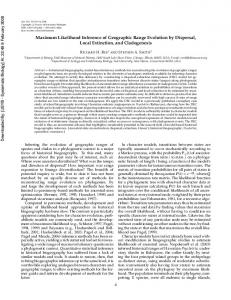
estimation technique described by Rousseeuw and Leroy (1984), were used to produce the calibrated images, so that targets that show spectral changes through time (eg. shifting patterns of sand and shadow in bare sand targets) are down-weighted in the regression analysis. The calibrated imagery for August 1989 and September 1990 are shown in Figure 2.

Figure 2 Calibrated (i) 1989 and (ii)1990 Landsat images with bands 4, 5, 7 in R, G, B.

2.5

Digital elevation data

Digital contour data at ten and twenty metre contour intervals were obtained from the Department of Land Administration (DOLA), Western Australia. The contour data were gridded using spline interpolation (Mitasova and Mitas, 1993; Mitasova and Hofierka, 1993) to form digital elevation models (DEMs) for the Upper Blackwood catchment and the Frankland-Gordon catchment. Spline interpolation is preferred over other gridding procedures (such as triangular irregular networks or kriging) since the resulting DEMs can be processed to provide continuous slope and curvature attributes (Moore et al., 1991). 2.6

Water accumulation

Water or drainage accumulation models simulate a rainfall event and produce rough estimates of the subsequent flow of water across the landscape (O’Callaghan and Mark; 1984; Jensen and Domingue, 1988; Quinn et al., 1991 and Schultz, 1994). Jensen and Domingue (1988) defined water accumulation models by assigning each cell a value equal to the number of cells that flow to it.

12

O’Callaghan and Mark (1984) and Jensen and Domingue (1988) calculate accumulation using a map showing drainage direction. The map shows the direction in which a cell drains, according to the steepest downhill slope from the cell. Water accumulation models produced using this method are termed single-direction water accumulation models. Quinn et al. (1991) present a more general algorithm for calculating water accumulation. The multiple-direction water accumulation model assumes that water flows in all downhill directions, with the amount of flow proportional to the slope of the drainage. They discuss the sensitivity of extracted flow paths to the choice of algorithm used to calculate accumulation. The results suggest that the multiple-direction model “gives a more realistic pattern of accumulating area on the hillslope portion of the catchment, but once in the valley bottom tends to braid back and forth across the floodplain”. They also claim that the single-direction model is more suitable once the flow has entered the permanent drainage system. The drainage system examined by Quinn et al. (1991) showed well-defined channels. This differs from the drainage systems of the south west of Western Australia which consist of chains of salt lakes in broad valleys with very low gradients (Mulcahy, 1978). Single-direction flow paths are unsuitable for such systems where flow paths are not well defined (Caccetta, 1997). Caccetta (1997) presents a method for identifying and labelling flat areas so that they can be patched into the water accumulation model. Flat areas are subsequently labelled according to the number of boundary pixels that flow into the flat area. Multiple-direction water accumulation maps, with flat areas incorporated have been produced for the Upper Blackwood catchment and Frankland-Gordon catchment, using the methods presented by Caccetta (1997). The water accumulation map for the Ryan’s Brook subcatchment is shown in Figure 3(i). Since water accumulation is low on the top of hills and increases as water flows into the valleys and drainage systems, the accumulation maps are used as a continuous measure of landform.

13

2.7

Drainage slope

The DEMs have also been used to produce maps showing the steepest downhill slope from any pixel. The map showing downhill slope for the Ryan’s Brook subcatchment is shown in Figure 3(ii).

Figure 3 (i) water accumulation and (ii) downhill slope maps - increasing values are shown from black to white.

2.8

Discussion

This chapter has described the study areas used to assess methodologies for mapping salinity in this thesis and the ground data that are used to train the classifiers. The image data used and the pre-processing required for the image data to be analysed as multi-temporal sequences have also been described. In addition, this chapter has presented several data sets that can be derived from costeffective contour data and used as surrogates for landform. Water accumulation models are used as a continuous measure of landform, since values increase as landforms change from hilltops to slopes to valleys. Stratification of the water accumulation models provides discrete landform classes. Multiple-direction models are claimed to be more suitable for the Western Australian landscape, and these have been produced for the upper Blackwood and Frankland-Gordon catchments. Maps showing the steepest downhill slope for any pixel have also been produced.

14

3

Classification and accuracy assessment

3.1

Introduction

This chapter presents background material describing the classification problem and criteria for selecting a classifier. Classifier accuracy is an important consideration in the selection of a classifier. This is particularly true when addressing the first objective of the thesis, which aims to produce accurate maps of salinity. Resubstitution and cross-validation methods for assessing accuracy are described. Simple estimates of classifier accuracy, including overall accuracy and the Kappa statistic are described with the intention to show that the Kappa statistic provides a better measure of classifier accuracy than overall accuracy. This measure is adopted throughout the remainder of the thesis for comparing classifier accuracy. 3.2

Classification

Given a set of objects, X, where each object is described by a set of numerical measures or attributes, and has an associated class, the pattern classification problem is to determine the class of a new object given its attribute values. For an example that illustrates the construction of the classification problem, see Alder (1994). A classifier is a method for assigning a class to an object according to its attribute values. A classifier can be defined as a function d(x) defined on X such that for every x in X, d(x) = j, if and only if x has class j. A classifier partitions X into disjoint subsets where members of each subset have the same class. Usually, a subset T of X is used to train the classifier, and the aim is to determine the class of a new object. 3.3

Criteria for selecting a classifier

This thesis investigates the use of different classifiers for producing maps of salinity and predicted salinity risk areas. The selection of a ‘best’ classifier is dependent upon a number of factors. These include the accuracy of the salinity maps, the amount of human intervention and processing time required to train the classifier and the complexity of the classifier. The complexity of the classifier measures how well the classifier can be interpreted. This is particularly relevant if the classifier is being used for exploratory data analysis.

15

This thesis examines these criteria in different contexts. The first objective of this thesis stresses that classifier accuracy is the most important criteria for mapping and monitoring salinity. Consequently, the assessment of classifiers for mapping salinity is based entirely on classifier accuracy. The second objective of this thesis aims to produce a simple model for predicting salinity risk which can be interpreted in such a way that the processes causing salinisation can be better understood. This requires that the complexity of the classifier used to predict salinity risk areas be minimised. Consequently, classifier accuracy plays a less important role in the selection of a ‘best’ classifier. This section discusses methods for assessing the accuracy of a classifier such as crossvalidated individual class accuracies and Kappa values. These are used to assess classifier accuracy throughout the thesis. 3.4

Resubstitution and cross validation

Given a set of ground truth data, it would seem desirable to train a classifier using all of the available data. A commonly used method for assessing accuracy does just this: resubstitution estimates of classifier accuracy re-use the training data. That is, accuracy statistics are calculated using the same data that are used to train the classifier. Breiman et al. (1984, p. 41) assert that “resubstitution estimates are usually optimistic”. This leads to the generalisation problem: resubstitution gives little insight on how the classifier would perform on previously unseen data. One means of bypassing this problem is via the use of cross-validation. Cross-validation provides a method for assessing a classifier’s performance on unseen data, whilst retaining the use of the entire training set. Stone (1974) describes cross-validation as follows: In its most primitive but nevertheless useful form, it consists in the controlled or uncontrolled division of the data sample into two subsamples, the choice of a statistical predictor, including any necessary estimation, on one subsample and then the assessment of its performance by measuring its predictions against the other subsample

In this simplest form, the classifier is trained on a portion of the ground truth data, and accuracy is assessed on the remainder of the data. In this way, the accuracy of the classifier

16

is tested on unseen data, and the estimates of classifier accuracy are more realistic than resubstitution estimates. K-fold cross-validation (Schaffer, 1993) provides a methods for using all of the available data to train, yet still testing the classifier on unseen data. The ground truth data are divided into k sets of independent training and test data. Sites are randomly selected from the ground truth data, such that the first 1/kth of the data are assigned to the first test set, the second 1/kth of the data are assigned to the second test set, and so on. Thus, the test sets are completely independent of each other. For each test set, the remaining data are used to train the classifier, so that the test and training sets for each partition of the data are also independent. Accuracy statistics can then be calculated for each of the k cross-validation partitions, and averaged to give overall accuracy statistics. 3.5

Assessing accuracy

3.5.1

Overall accuracy

The accuracy of a classification has traditionally been measured by the overall accuracy. However, as a single measure of accuracy, the overall accuracy (or percentage classified correctly) gives no insight into how well the classifier is performing for each of the different classes (Fitzgerald and Lees, 1994). In particular, a classifier might perform well for a class which accounts for a large proportion of the test data and this will bias the overall accuracy, despite low class accuracies for other classes. This can be seen in chapter 5, where nonsaline training sites outnumber the saline training sites, and the decision tree classifiers tend to map non-saline areas with higher accuracy than the saline areas. Reducing the number of non-saline training sites to equal the number of saline training sites would eliminate the bias, but would also reduce the non-saline class accuracy, thus reducing overall accuracy. To avoid such a bias when assessing the accuracy of a classifier, it is important to consider the individual class accuracies. In this application, this is reasonable since there are only two classes. Individual class accuracies are quoted for each of the classifiers assessed in this thesis.

17

3.5.2

The Kappa statistic

The Kappa statistic was derived to include measures of class accuracy within an overall measurement of classifier accuracy (Congalton, 1991). It provides a better measure of the accuracy of a classifier than the overall accuracy, since it considers inter-class agreement (Fitzgerald and Lees, 1994). It is used to assess the accuracy of a classifier against known validation data. The Kappa statistic is calculated from the error matrix in the following manner. Label each entry in the error matrix as p ij where i denotes the row number and j denotes the column number. Then the class accuracies are calculated by taking the row totals p io and dividing by the number of test sites, N. Denote the column totals by p oj. Thus the error matrix and totals are:

p1,1 . p i,1 p o,1 The proportion of overall agreement po = agreement p c =

∑p

i =1, N

io

... ... ... ...

p1, j . pi, j p o, j

∑p

i =1 , N

ii

p1, o . pi ,o N

and the proportion of chance expected

p oi are used to calculate the Kappa statistic:

p − pc Kˆ = o . 1 − pc The Kappa statistic is used to test the null hypothesis that there is no agreement between the two classifiers, ie. H0: K=0. The standard error of the Kappa statistic is given by:

  1 2 se( Kˆ ) =  po + pc − ∑ pio poi ( pio + poi )  (1 − pc ) N  i =1, N 

1

2

The null hypothesis is tested by converting the Kappa statistic to the standard Z score (Z = K / SE(K) ) and testing against the standard Gaussian distribution.

18

The Kappa statistic has been used to compare the accuracy of several classifiers (Congalton, 1991; Fitzgerald and Lees, 1994), since it measures the difference between each classifier and the ground truth. 3.5.3

Other methods for assessing accuracy

More sophisticated measures of classifier accuracy are presented by Fienberg (1970, 1978) and Zhuang et al. (1995). Feinberg describes the use of loglinear models for analysing contingency tables. Contingency table analysis can be used to consider questions like: •

Are the labels produced by a classifier independent of the subset of training data used?

•

Does a classifier perform consistently over the different partitions of ground truth data?

•

Do the classifiers perform differently?

Software packages, such as CoCo (Badsberg, 1995) and Splus, can be used to selectively fit contingency models and choose the most appropriate. Zhuang et al. (1995) model the performance of the classifiers as five replications (over the five train / test partitions) of a two-factor experiment with one observation per entry. Their method can be viewed as a simplified contingency table analysis. 3.6

Discussion

This chapter has defined the classification problem. Later chapters will investigate various algorithms for producing classifiers, and examine the accuracy with which these methods can be used to map and predict salinity. This chapter has shown that the Kappa statistic provides a useful simple measure of classifier accuracy. This method for assessing accuracy will be adopted throughout the remainder of the thesis. For each classifier investigated, the individual class accuracies will also be quoted, so that the errors of omission and commission can be determined. Error of omission are given by the proportion of saline areas that are mapped as non-saline; whilst errors of commission are the proportion of non-saline areas are mapped as saline. These errors describe the degree to which the classification is under-estimating and over-estimating salinity.

19

4

Maximum likelihood classification

4.1

Introduction

This chapter examines the use of maximum likelihood classification for producing salinity maps from a single Landsat image. Maximum likelihood classification has traditionally been used as a baseline for the classification of remotely sensed data. For instance, Apan (1997) uses maximum likelihood classification to assess the utility of Landsat data for mapping forest rehabilitation and Basham May et al. (1997) use maximum likelihood classification to compare the effectiveness of Landsat and SPOT data for vegetation classification. This chapter uses maximum likelihood classification to form a baseline against which the results achieved using other classifiers can be compared. Section 4.2 presents the background to maximum likelihood classification and neighbourhood modifications to the maximum likelihood classifier. Section 4.3 presents the results of classification of four Landsat images using maximum likelihood techniques, and using neighbourhood-modification to the maximum likelihood procedure. Section 4.4 discusses the results of the chapter. 4.2

Maximum likelihood classification

Maximum likelihood classification is based upon the assumption that there exist statistical models describing the distribution of the classes in the attribute space. Given these models, the class of a new object is determined by calculating which of the models is more likely to describe that object. In other words, the model with maximum likelihood is selected. Maximum likelihood classification usually assumes multivariate normal (Gaussian) models. For a set of M n-dimensional objects, (x1,...xM) where xi = (x1,1,....x1,n)T, the Gaussian probability density function (pdf) is defined to be

g [ m, C ] =

−( x −m )T C −1 ( x − m )

1 ( 2)

n

det(C )

2

e

,

where the vector of means, m, is given by

m=

1 M

M

∑x

i

i =1

20

and the covariance matrix, C, is given by

C=

M 1 T ( xi − m)( x i − m) . ∑ ( M − 1) i=1

The matrix C is positive semi-definite and symmetric by construction. Hence, it is possible to diagonalise the matrix and calculate the eigenvalues and eigenvectors. In the case where the attribute space is two-dimensional, the eigenvalues and eigenvectors provide a useful means for displaying the two-dimensional Gaussian as an ellipse in the attribute space. By writing

 λ 0  e  C = ( e1 , e 2 )  1  1  ,  0 λ 2  e 2  where e1 and e2 are the eigenbasis vectors, and λ1 and λ 2 are the eigenvalues of C. Then the ellipse which marks all points in the attribute space that are two standard deviations away from the mean is given by

  2 λ1 0  e  cos( t )  2 1       [ ]  x ∈ ℜ : x = m + (e1 , e 2 )  e  sin( t ) , t ∈ 0,2π  .  0 2 λ     2  2   Consider a simple example, illustrated in Figure 4 (overleaf). Each object has two attributes and belongs to one of two classes. The training set consists of 40 objects, plotted as squares or triangles according to the class to which objects belong. The fitted two-dimensional Gaussian distributions are shown in colour. The class of a new object can be determined by measuring the distance of the object from the fitted Gaussian distributions. An overlap area exists, within which the class of a new object may be in doubt. 4.2.1

Bayes’ theorem and maximum likelihood classification

Bayes’ theorem provides a framework for allocating probabilities of class labels for a new object. For instance, an object located in the overlap region of the attribute space shown in Figure 4 may belong to class 1 with a probability of 0.55 and belong to class 2 with probability of 0.45. Bayes’ theorem requires that we know the prior probability of any object belonging to each of the classes. That is, the proportion of objects belonging to each class over the population. The probability for class Ck is written P(Ck). Given a set of attribute values, we can form the joint probability P(Ck, x), or the probability that an object has attribute values 21

given by x and belongs to class Ck. Then the conditional probability P(x | Ck) is the probability that the object has attribute values equal to x given that it belongs to class Ck.

Figure 4 Fitted Gaussian distributions.

Probability theory states: P(Ck, x) = P(x | Ck) P(Ck). Bayes’ Rule can then be applied to give:

P(C k | x) =

P( x | C k ) P( C k ) . P (x )

The probability P(Ck | x) is called the posterior probability of the object belonging to class Ck given that it has attribute values x. Maximum likelihood classification uses the estimated Gaussian distribution to calculate the posterior probabilities for each class, and assigns a new object to the class with the highest posterior probability.

22

4.2.2

Canonical variate analysis

Canonical variate analysis provides a method for transforming input attribute data in such a way that the separation between training classes is maximised. Plots of canonical variate means (see section 4.3.2) for the training sites provide a simple tool for examining the separability of the classes. Canonical variate analysis can be considered as a two-stage rotation of the attribute data (Campbell and Atchley, 1981). The first stage consists of a principle component analysis (Richards, 1986, pp. 127-130) of the attribute data. The second stage consists of an eigenanalysis of the group means for the principle component scores from the first stage. In this way, the differences between the classes are maximised relative to the differences within the classes. This is particularly relevant to remote sensing applications where training sites are composed of regions of many pixels since the spectral values of pixels belonging to the same training site may cover a range of values. Given g classes, each with n g training objects such that xki = (xi,ki ,…,xM,ki ) for all k=1,…,g and i=1,…,nk then a canonical variate analysis forms a linear combination, y ki = c T x ki , of the input attributes such that the ratio of the between-groups sum of squares, g

SSB = ∑ nk ( yk − yT )2 , k =1

and the within-groups sum of squares, g

nk

SSW = ∑ ∑ ( y ki − y k ) 2 , k =1 i =1

where y k =

1 nk 1 y ki is the mean of the k-th class, yT = ∑ nT n i=1

g

∑n y k

k

is the overall mean and

k =1

g

nT = ∑ nk is the total number of training objects. k =1

Substituting y ki = c T x ki gives g

nk

SSW = c T ∑ ∑ ( xki − xT )( xki − x T )T c k =1 i =1

= c Wc T

23

and g

SSB = cT ∑ nk ( x k − xT )( x k − x T ) T c k =1

= c Bc. T

Thus, maximising f =

SS B c T Bc = requires an eigenanalysis Bc=Wcf. SSW c TWc

Given p attributes, there are h=min(p, g-1) canonical vectors with non-zero canonical roots. If C=(c1,…c h) and F=diag(f 1,…f h) then the eigenanalysis becomes BC=WCF.

4.2.3

Neighbour-modified maximum likelihood classification

Since areas with a particular ground cover type are generally contiguous and smoothly bounded, it is likely that the ground cover at any pixel is influenced by the ground cover at the pixels surrounding it. Maximum likelihood classifications of Landsat data can be modified to include neighbourhood information via the use of Markov random fields to model the class labels (Karssemeijer, 1990; Geman and Geman, 1984; Besag, 1986). The method adopted in this thesis is that of Kiiveri and Campbell (1992). The following paraphrases their work. If we assume that: 1. The probability of any label is dependent only on the labels of its neighbours, and 2. The probability of the spectral values of a pixel is dependent only on the spectral values of its neighbour and the labels of the pixel and its neighbours. That is, the labels are assumed to be realisations from a Markov Random Field (Besag, 1986). Then, Bayes Rule implies that the probability of any label given the image data depends only on the neighbourhood labels and the image data in the neighbourhood including the centre pixel. Kiiveri and Campbell (1992) show that neighbourhood modifications to the maximum likelihood classifier, where the standardised variables are assumed to be modelled by a multivariate conditional autoregressive (CAR) model, involves two steps:

24

1. Calculation of the (Mahalanobis) distance using the standardised variable that has been neighbourhood-corrected. 2. Adjusting the label according to the labels of neighbouring pixels. Using a cyclic ascent algorithm (Besag, 1986) to update the label at any pixel involves choosing the class with the minimal neighbour-adjusted distance. 4.3

Maximum likelihood classification of the Landsat data

The Landsat images were classified into major ground cover types using maximum likelihood classification. These classification maps serve as a comparison for the decision tree and neural network classifications described in chapters five and 6. 4.3.1

Selection of training sites

Training sites for the Landsat classification were digitised using the yearly images as bases. Only sites from the Blackwood catchment were selected so that the Ryan’s Brook ground truth data could be retained as independent validation data. The sites were selected to include the following ground cover types: water, healthy remnant vegetation, poor remnant vegetation, bare salt scalds, salt-affected land vegetative cover (such as trees or other salttolerant species), bare soil, crops (such as canola, lupins, wheat, oats or barley), and pastures. 4.3.2

Canonical variate analyses

Canonical variate analyses (see section 4.2.2) were conducted for each Landsat image. The canonical variate plots of the first canonical mean against the second canonical mean for each training site are shown in Figures 5 to 8. These plots show that the training sites corresponding to different ground cover types are clustered; however, there is a good degree of overlap between the different cover types.

25

Figure 5 Canonical variate plot for August 1989.

The canonical variate plot for 1989, shown in Figure 5, shows an overlap region that contains saline sites, bare soil and agricultural land. Similar overlap regions can be noted in each of the canonical variate plots. The agricultural sites contained in this region have been inspected in the Landsat images; they tend to be cropped or pastured areas where growth is poor because of late germination, poor conditions or management effects. A mixed class has been included in the maximum likelihood classifications to cover this region in the canonical variate space. The plots also show that some saline sites are spectrally similar to bare soil sites and other saline sites are spectrally similar to remnant vegetation sites. These overlap regions are reflected in the classification statistics discussed in the section 4.3.3.

26

Figure 6 Canonical variate plot for September 1990.

Figure 7 Canonical variate plot for September 1993.

27

Figure 8 Canonical variate plot for August 1994.

4.3.3

Classification accuracies

The images have been classified using maximum likelihood classification (see section 4.2) into six broad classes: salt, mixed, bare soil, bush, agricultural land and water. The classification maps for August 1989 and September 1990 are shown in Figure 9. Visual examination shows that the 1989 classification tends to over-estimate salinity, frequently mapping agricultural areas with poor ground cover as salt-affected. This can be seen when the classification map in Figure 9 (i) is compared to the calibrated image in Figure 2 (i). In the calibrated image, pastures can be recognised by orange colours while salt-affected areas appear grey. Some areas classified as salt can be clearly seen to be pastures in the image. Other areas that have been mapped as salt can be recognised as remnant vegetation by the straight edges in their outline. The 1990 classification maps a much smaller proportion of the image as salt; this is possibly caused by the differences in scene brightness between the two years. It can be seen in the calibrated image data (Figure 2) that the 1989 image is considerably darker in colour. This reflects seasonal differences: the rainfall data for the region show that 1989 was a wetter year than 1990.

28

Figure 9 (i) 1989 and (ii) 1990 Landsat classifications.

Classification accuracies were calculated over independent validation data from the Ryan’s Brook subcatchment. The classification accuracies over the validation data are shown in Tables 1 to 4. The percentage of accurately classified sites for each class is shown in the final row of the tables. This value represents the proportion of each true class that was classified correctly. Table 1 1989 classification statistics.

Image Label salt mixed bare soil bush crop/pasture water accuracy Kappa

Ground truth salt not salt 769 965 6 112 1 116 161 995 258 2199 0 13 0.6425 0.7550 0.3643

Table 2 1990 classification statistics.



Each of the Landsat image classifications showed large errors of omission (35-50%) and errors of commission (26-35%) when mapping salinity. That is, saline areas were mapped as non-saline and non-saline areas were mapped as saline. The errors are reflected in the low Kappa values.

29







Examination of the classifications at the saline ground sites showed that none of the sites was entirely incorrectly classified - only pixels within the sites and on the edges of the saline sites were erroneously labelled as other than salt. This suggests that some errors of omission might be cleared up by neighbourhood-modifications to the maximum likelihood classifier. The results of applying the neighbourhood-modifications are described in the next section. 4.3.4

Neighbourhood-modified classification

Neighbourhood modified maximum likelihood classifications (as described in section 4.2.3) have been produced for the Ryan’s Brook study area. The results are shown in Tables 5 to 8. The errors of omission (for mapping salinity) have been reduced by 10-20% for each year and the Kappa values improved with the inclusion of neighbourhood effects. Figure 10 shows the neighbourhood-modified classifications for August 1989 and September 1990. The smoothing effects of the neighbourhood modifications can be seen when Figure 10 is compared with Figure 9; however some of the errors noted in the previous classifications (section 4.3.3) can still be seen in the neighbourhood-modified classification maps. For instance, the 1989 map over-estimates salinity and the two maps look very different given that changes in salinity are unlikely to have occurred within the time period.

30

Table 5 1989 neighbourhood-modified classification statistics.












Figure 10 Neighbourhood-modified classifications for (i) 1989 and (ii) 1990.

31

4.4

Discussion

This chapter has examined the use of maximum likelihood classification for producing salinity maps, each using a single date of Landsat imagery. Training sites were selected to cover a range of land cover. Canonical variate analyses were conducted to examine the spectral separability of the training sites and for each date, overlap areas between classes could be seen between data clusters corresponding to the different land cover types. Classification of the images into six classes, including a mixed class, showed poor results. The errors of omission for mapping salinity, or the proportion of saline validation sites erroneously labelled as not salt, ranged from 35-50% for the four classifications. In addition, 26-35% of the non-saline validation sites were erroneously labelled as salt. The low class accuracies were reflected by the Kappa values, which ranged from 0.2871 to 0.3927. Neighbourhood modifications to the maximum likelihood classifications improved the Kappa values to between 0.4255 and 0.5411; however, between 22-38% of the saline validation sites were still omitted and between 14-23% of the non-saline validation sites are mapped as saline. The accuracies of the maximum likelihood classifications thus remain poor. The classified land cover maps shown in Figures 9 and 10 show that: 1. A greater proportion of the image is mapped as saline in 1989 than in 1990, despite it being unlikely that on-ground changes have occurred within this time period. 2. Many areas mapped as salt seem to occur outside of the valleys where salinity is more likely to occur; this can be justified by comparing the classifications with the water accumulation map shown in Figure 3. It is proposed that combining the Landsat image data from 1989 and 1990 may improve the accuracy for mapping salinity for the time period (effectively removing the inconsistencies noted in the first observation above). In addition, landform information may further improve accuracy by minimising errors of the type noted in the second observation. Maximum likelihood procedures do not provide an effective framework for combining disparate data sets such as these because it becomes difficult to assume a known joint probability distribution between the spectral data and other spatial data sets. Non-parametric classifiers provide a means for classification where the distribution is unknown. For this

32

reason, the following two chapters examine the use of non-parametric decision tree and neural network classifiers for integrating several successive seasons of Landsat imagery with landform attributes derived from digital elevation models for mapping salinity.

33

5

Decision trees

5.1

Introduction

The previous chapter examined the use of maximum likelihood techniques for classifying single Landsat images to produce maps showing areas affected by salinity. The chapter concluded that including Landsat data for an additional season and information about landform might reduce errors of the type noted in the maximum likelihood classifications. Since maximum likelihood procedures do not provide an effective framework for integrating remotely sensed data with other spatial data, it is proposed that non-parametric classifiers, such as decision trees, are required. Decision tree classifiers provide a non-parametric means for integrating Landsat imagery with landform to produce maps of salinity. Decision trees have two advantages (see section 1.1): 1. They enable relationships between the Landsat data and terrain data to be extracted without prior knowledge about the ways in which these data interact. 2. They provide a means to automatically partition the attribute space into subregions corresponding to subclasses of the broader classes of interest. To date, few studies have investigated the use of decision trees for the classification of remotely sensed data. Lees and Ritman (1991) examined the use of decision trees for mapping vegetation species using Landsat and other spatial data. Byungyong and Landgrebe (1991) used decision trees to classify AVIRIS data. Eklund et al. (1994) used a decision tree approach to assess the effect of incremental data layers on groundwater recharge estimates. They examined whether including additional information provided by ground-based electromagnetic measurements provided more accurate recharge estimates than using Landsat and other spatial data. A recent study by Friedl and Brodley (1997) showed that decision tree algorithms consistently outperformed maximum likelihood techniques when classifying spectral data. They noted, however, that decision tree algorithms tend to optimise overall classification accuracy at the expense of smaller classes. For this reason, the methods used to assess the accuracy of a

34

classifier must be carefully selected. Chapter 3 of this thesis discussed the accuracy assessment methods adopted for this study. This chapter investigates the use of decision tree classifiers for integrating two successive dates of Landsat imagery with landform attributes to produce maps of salinity. Background material about decision tree classifiers and the particular induction algorithms investigated is presented in section 5.2. Section 5.3.1 discusses the selection of input attributes, using several induction algorithms. The attribute set is then used, in section 5.3.2, to compare two induction algorithms with various input options. The most accurate decision tree classifier is selected by using 5-fold cross-validated class accuracies and Kappa values. 5.2

Decision tree classification

A decision tree classifier is a hierarchical structure where at each level, a test is applied to one or more attribute values that may have one of two outcomes. The outcome may be a leaf, which allocates a class, or a decision node, which specifies a further test on the attribute values and forms a branch or subtree of the tree. Classification is performed by moving down the tree until a leaf is reached. The structure of a decision tree classifier is shown below in Figure 11.

Figure 11 The decision tree structure.

The method for constructing a decision tree as paraphrased from Quinlan (1993, pp. 17-18), is as follows: 35

If there are k classes denoted {C1, C2,...,Ck}, and a training set, T, then •

if T contains one or more objects which all belong to a single class Cj,, then the decision tree is a leaf identifying class Cj.

•

if T contains no objects, the decision tree is a leaf determined from information other than T.

•

if T contains objects that belong to a mixture of classes, then a test is chosen, based on a single attribute, that has one or more mutually exclusive outcomes {O1, O2,..., On}. T is partitioned into subsets T1, T2,..., Tn, where Ti contains all the objects in T that have outcome Oi of the chosen test. The same method is applied recursively to each subset of training objects.

Quinlan’s decision tree classifier, c4.5, uses tests based on a single attribute value. That is, decision boundaries are parallel to the attribute axes, such as the decision regions shown in Figure 12 (i). Other tree classifiers may use more than one attribute value. For instance, CART, developed by Breiman et al. (1984), can perform tests based on a linear combination of continuously-valued attributes, and oc1, by Murphy et al. (1994), was designed specifically to produce decision trees with oblique (linear) decision boundaries like those shown in Figure 12 (ii).

Figure 12 Given axes that show the attribute values and colours corresponding to class labels (i) axis-parallel and (ii) oblique decision boundaries.

Oblique decision boundaries can be an advantage in examples such as that shown in Figure 12 where the natural class regions can be approximated using only 3 oblique decision boundaries compared to 19 axis-parallel boundaries.

36

5.2.1

Criteria for evaluating splits

Decision tree classifiers differ in the ways they determine how to partition the training sample into subsets and thus form subtrees. That is, they differ in their criteria for evaluating splits into subsets. The c4.5 induction algorithm uses information theory (Shannon, 1949) to evaluate splits. Two splitting criteria are implemented. The gain criterion (Quinlan, 1993, ) is developed in the following way: For any subset S of X, where X is the population, let freq(j i,S) be the number of objects in S which belong to class i. Then consider the ‘message’ that a randomly selected object belongs to class j i. The ‘message’ has probability freq(j i,S) / |S|, where |S| is the total number of objects in subset S. The information conveyed by the message (in bits) is given by -log2 (freq(j i,S) / |S|). Summing over the classes gives the expected information (in bits) from such a message:

info(S) = − log 2 (

freq(C j , S ) S

) .

When applied to a set of training objects, info (T) gives the average amount of information needed to identify the object of a class in T. This amount is also known as the entropy of the set T. Consider a similar measurement after T has been partitioned in accordance with the n outcomes of a test X. The expected information requirement can be found as a weighted sum over the subsets {TI}: n

Ti

i =1

T

infoX (T ) = ∑

. info(Ti ) .

The quantity gain (X) = info (T) - infoX (T) measures the information that is gained by partitioning T in accordance with the test X. The gain criterion (Quinlan, 1993) selects a test to maximise this information gain. 37

The gain criterion has one significant disadvantage in that it is biased towards tests with many outcomes. The gain ratio criterion (Quinlan, 1993) was developed to avoid this bias. The information generated by dividing T into n subsets is given by n

split info (X) = ± ∑ i =1

 Ti  . . log 2   T T  

Ti

The proportion of information generated by the split that is useful for classification is gain ratio (X) = gain (X) / split info (X). If the split is near trivial, split information will be small and this ratio will be unstable. Hence, the gain ratio criterion selects a test to maximise the gain ratio subject to the constraint that the information gain is large. This compares with CART’s impurity function approach (Breiman et al., 1984), where impurity is a measure of the class mix of a subset and splits are chosen so that the decrease in impurity is maximised. This approach led to the development of the gini index (Breiman et al., 1984). The impurity function approach considers the probability of misclassifying a new sample from the overall population, given that the sample was not part of the training sample, T. This probability is called the misclassification rate and is estimated using either the resubstitution estimate (or training set accuracy), or the test sample estimate (test set accuracy). The node assignment rule selects i to minimise this misclassification rate. In addition, the gini index promotes splits that minimise the overall size of the tree. 5.2.2

Tests on continuous attributes

The algorithm for finding appropriate thresholds for continuous attributes (Paterson and Niblett, 1982, Breiman et al., 1984, and Quinlan, 1993) is as follows: The training objects are sorted on the values of the attribute. Denote them in order as {v1, v2,...,vm}. Any threshold value lying between vi and vi+1 will have the same effect, so there are only m-1 possible splits, all of which are examined.

38

5.2.3

Tests on linear combinations of continuous attributes

Oblique decision trees perform tests on a linear combination of p attribute values, so the test at each node takes the form: p

∑a x +a i i

i =1

p +1

> 0,

where a1 ,..., a p+1 are real-valued coefficients. Given a set of attributes, it is possible to choose the optimal split on a single attribute by searching through all possible splits. Determining the optimal linear combination of input attributes on which to split (using a particular splitting criteria such as those described in section 5.1.1) requires a heuristic search algorithm. The algorithm employed by CART is based on hill climbing (ie. maximising the goodness of the split) and then backward elimination of irrelevant attributes (Breiman et al., 1984). This algorithm is refined by Murphy et al. (1994) by the addition of a random jump procedure and local perturbations that aim to avoid the algorithm stopping at local minima. 5.2.4

Pruning

Decision tree classifiers aim to refine the training sample T into subsets which have only a single class. However, training samples may not be representative of the population they are intended to represent. In most cases, fitting a decision tree until all leaves contain data for a single class causes over-fitting. That is, the decision tree is designed to classify the training sample rather than the overall population and accuracy on the overall population will be much lower than the accuracy on the training sample. C4.5, CART and oc1 all grow trees to maximum size, where each leaf contains single-class data or no test offers any improvement on the mix of classes at that leaf, and then prune the tree to avoid overfitting. Pruning occurs within c4.5 when the predicted error rate is reduced by replacing a branch with a leaf. CART and oc1 use a proportion of the training sample to prune the tree. The tree is trained on the remainder of the training sample and then pruned until the accuracy on the pruning sample can not be further improved.

39

5.3

Mapping salinity using decision trees

This section aims to compare different decision tree classifiers for mapping areas affected by salinity. The classifier c4.5 is used to produce decision tree classifications using various parameter settings for pruning and the minimum number of training cases required to be classified at any leaf of the tree. The oc1 induction algorithm is used in both axis-parallel mode and oblique mode, using each of the available splitting criteria ∗ .

5.3.1

Attribute selection

The selection of input attributes for training classifiers was based upon methods used to prepare maps of salinity in the Kellerberrin and Esperance regions in WA (Furby et al., 1995). That study showed that at least two years of Landsat imagery combined with landform information were required to adequately map salinity. The results of chapter 4 showed that salinity could be mapped with, at most, 78% accuracy using neighbourhoodmodified maximum likelihood techniques to classify image data from a single date. The set of twelve input attributes used in this study include Landsat bands 1, 2, 3, 4, 5 and 7 for August 1989 and September 1990 images, water accumulation (logarithmic scale) and downhill slope. To determine whether appropriate subsets of the input attributes were preferable for mapping salinity, decision trees were produced using five subsets of the attribute data: 1. August 1989 Landsat data only. 2. August 1989 Landsat data and landform attributes. 3. September 1990 Landsat data only. 4. September 1990 Landsat data and landform attributes.

∗

Since oc1 replicates the methods implemented in CART when used with the gini criterion, CART is

not tested explicitly. The oc1 implementation of oblique splits using the gini criterion differs from CART’s implementation; oc1 can be used to implement CART’s search mechanism but this has not been tested in this thesis.

40

5. All attributes.

Since c4.5 and oc1 perform splits differently, it is possible that c4.5 might perform best on one set of input attributes, while oc1 might perform best on a different set. For this reason, both decision tree classifiers have been used to determine the input attributes required for mapping salinity; however, only the default input options were used and oc1 was implemented using only the gini criterion. Attribute sets were assessed using both axis-parallel and oblique modes. Class accuracies and Kappa values were calculated for each of the five cross-validation partitions, and averaged to produce the values shown in Tables 9 to 11.

Table 9 C4.5 accuracies and Kappa values averaged over 5 partitions.

attribute set 1 2 3 4 5

not salt accuracy 0.9131 0.9298 0.9139 0.9187 0.9233

salt accuracy 0.6708 0.7421 0.6218 0.6979 0.7620

Kappa 0.5764 0.6641 0.5406 0.6092 0.6685

Tables 9 shows that the most accurate result achieved using c4.5 (according to the Kappa value) are achieved when the entire set of input attributes is used. However, the accuracy is only slightly reduced when the September 1990 image data are removed from that set. The maximum tree depth over the five partitions was 29 when all input attributes were used, and 28 without the September 1990 image data, showing no simplification of the tree was gained by excluding the 1990 Landsat data. Table 10 shows that the most accurate result using oc1 in axis-parallel mode (using the gini criterion to assess splits) is achieved when the entire set of input attributes is used. The next best accuracy is achieved when the August 1989 image data are removed from that set. This differs from the c4.5 results, implying that the different tree-growing procedures prefer different subsets of input attributes. The maximum tree depth was 15 when all input attributes were used and 19 when the August 1989 image data were removed, showing that the removal of six bands of Landsat data did not simplify the decision tree.

41

Table 10 Oc1 (axis-parallel) accuracies and Kappa values averaged over 5 partitions.



salt accuracy 0.6588 0.6677 0.6340 0.7119 0.7557

Kappa 0.5936 0.5971 0.5585 0.6207 0.6876

Table 11 shows that the most accurate result achieved using oc1 in oblique mode (using the gini criterion to assess splits) is also achieved when the entire set of input attributes is used.

Table 11 Oc1 (oblique) accuracies and Kappa values averaged over 5 partitions.



salt accuracy 0.6318 0.6699 0.5740 0.6556 0.7199

Kappa 0.5816 0.6061 0.5295 0.5932 0.6532

These results have shown that all 14 attributes are required to produce the most accurate decision tree classifications using c4.5 or oc1 in axis-parallel or oblique modes. Comparisons of classifiers using all input attributes are presented in the following section. 5.3.2

Decision tree accuracies for mapping salinity

Decision trees have been produced using the entire set of attributes. C4.5 has been used with six sets of input parameters; these are described by Quinlan (1992). The -c option affects the amount of pruning done: smaller values produced more highly pruned trees. The -m option defines the minimum number of training cases that can be classified by any leaf of the tree (thus also affecting pruning). The oc1 classifier has been used with each available splitting criterion (gain ratio, gini, twoing, maximum minority, sum minority and variance) in both axis-parallel and oblique modes.

42

Table 12 C4.5 accuracies and Kappa values averaged over 5 partitions.

Input parameters default -c10 -c10 -m10 -c5 -c5 -m10 -m10

not salt accuracy 0.9512 0.9622 0.9329 0.9082 0.9112 0.9130

salt accuracy 0.6982 0.7728 0.7764 0.8009 0.8347 0.7729

Kappa 0.6852 0.7624 0.7101 0.6777 0.6928 0.6476

Table 12 shows the class accuracies and Kappa values achieved using different input parameters to c4.5. The table shows that the most accurate result was produced using option –c10. It is important to note that the statistics shown are averaged over five different crossvalidation partitions. That is, decision trees are trained using five different training sets and accuracies are calculated over five independent test sets. For each of the parameter settings tabled, five different decision trees are produced. This raises two important issues. First, how different are the decision trees produced using the different partitions, and second, which tree should be used to produce the classification map? By examining the accuracy statistics for each partition, this thesis attempts to highlight the problem of classifier choice when crossvalidation is employed for accuracy assessment. The Kappa values for each partition are shown in Table 13.

Table 13 Kappa values for each cross-validation partition.

Input parameters default -c10 -c10 -m10 -c5 -c5 -m10 -m10

Partition 1

Partition 2

Partition 3

Partition 4

Partition 5

0.6930 0.6689 0.7133 0.6294 0.6254 0.6409

0.6924 0.7347 0.7040 0.5798 0.9202 0.6493

0.6689 0.7656 0.9041 0.6040 0.6155 0.6375

0.7065 0.6905 0.6251 0.9113 0.6610 0.6481

0.6651 0.9521 0.6040 0.6639 0.6421 0.6625

It should be noted that some of the input parameter settings can result in very different Kappa values across partitions. For instance, option –c10 achieves a much higher accuracy for partition 5 than any other partition, options –c10 –m10 achieve a much higher accuracy for partition 3 than any other partition and options –c5 –m10 achieve a much higher accuracy for partition 2 than any other partition. It is concluded that different input parameters perform 43

differently for different subsets of the ground data. Each of the cross-validated training samples must, by construction, contain at least 75% of the object contained in another of the training samples (see section 3.4). Thus, it is also concluded that the decision tree classifiers are susceptible to large variations in accuracy when only small changes are made to the composition of the training sample. Having recognised that the use of cross-validation for accuracy assessment can provide the user with further issues about classifier selection, this thesis takes the view that 5-fold cross validation can be used to compare the performance of the different classifiers using various input attributes, but that the final classifier should be trained using all of the available data. This view is taken for convenience, so that comparisons of classifier accuracy can be made. However, it should be noted that it is a naive opinion, since it assumes that the classifier will perform better given a larger training sample. This assumption is not supported by researchers into the use of ensembles of classifiers (Dietterich, 1997). Ensembles of classifiers (or hybrid classifiers) combine the results of applying several different classifiers to a problem. For instance, each of the decision trees produced using the five cross-validation sets might be used to assign a class to a particular object. The class labels might then be combined using weighted averages or more sophisticated means, to produce a final class label for the object. Such a system has been named a cross-validated committee by Parmanto et al. (1996). This issue is discussed further in chapters 6 and 9 of the thesis. Figure 13 shows the salinity map produced using the options to c4.5 that gave the highest Kappa value. All of the available training data were used to train the decision tree using those options. Classification maps were produced in this manner for each of the classifiers assessed using cross-validated accuracies. Errors in the c4.5 salinity map tend to be areas of remnant vegetation or agricultural land that have been mapped as saline; that is, saline areas that have been over-estimated. This can be seen when Figure 13 is compared with the calibrated Landsat images shown in Figure 2 which shows that saline regions are largely constrained within valley floors. This indicates that the decision trees are using the landform attributes in an appropriate manner. However, many isolated pixels are mapped as saline. Given that saline regions are usually contiguous, this means that isolated pixels mapped as salt are more likely not salt-affected.

44

Figure 13 Salinity map produced using c4.5.

Decision trees were trained using each of the criteria available with the oc1 classifier, in both the axis-parallel mode and the oblique mode. Table 14 shows that the highest accuracy was achieved when the axis-parallel mode was used with the gain ratio criterion. The oc1 implementation of the gain ration criterion differs from the c4.5 implementation only by the pruning algorithms. Table 14 Oc1 accuracies and Kappa values averaged over 5 partitions.

criterion gain ratio gain oblique gini gini oblique twoing twoing oblique max minority max oblique sum minority sum oblique variance var oblique

not salt accuracy 0.9336 0.9280 0.9362 0.9330 0.9362 0.9181 0.9366 0.9374 0.9956 0.9748 0.9362 0.9279

salt accuracy 0.7651 0.7158 0.7557 0.7199 0.7557 0.6960 0.6445 0.6359 0.1207 0.3575 0.7557 0.7017

Kappa 0.6896 0.6425 0.6876 0.6532 0.6876 0.6113 0.6037 0.5895 0.1697 0.4057 0.6876 0.6300

The oc1 implementation of the gini criterion emulates the CART decision tree classifier, and produces similar results to the gain ratio criterion. Figure 14 shows the most accurate salinity map produced using the oc1 implementation of the gain ratio splitting criterion with axisparallel splits.

45

These results suggest that producing decision trees that split on linear combinations of input attribute data provides little advantage over splitting on single attribute values. In most cases, the depth of oblique decision trees is lower than for axis-parallel trees; however, the amount of time required to derive the trees from training data is was noted to be far greater. The resulting accuracies are slightly lower for each of the implemented splitting criteria.

Figure 14 Salinity map produced using oc1.

5.4

Discussion

This chapter has examined the use of decision tree classifiers for mapping salinity from two successive seasons of Landsat imagery and DEM-derived landform attributes. Two decision tree algorithms have been tested: c4.5 and oc1, which replicates the splitting criteria used by c4.5 and CART, along with other splitting criteria. The accuracy achieved using c4.5 (summarised using the Kappa value) ranged from 0.6476 to 0.7623. In axis-parallel mode, oc1 achieved Kappa values ranging between 0.2697 using the sum minority criterion and 0.6896 using the gini criterion. For each of the splitting criteria implemented by oc1, the oblique version performed less accurately. The most accurate decision tree was produced using c4.5 with options -c10 (a moderate level of pruning), showing an marked improvement on the results achieved by the single-date Landsat maximum likelihood classifiers. In addition, the amount of time required to select training sites for the classifications was vastly reduced. Using the decision tree classifiers, training classes could be reduced to just

46

two (salt and not salt) rather than the many different cover classes identified in section 4.2.1 for training the maximum likelihood classifiers. The classification map produced using the most accurate decision tree (Figure 13) shows contiguous regions of salt, located in the valleys, and smaller regions of salt, located away from the valleys. This is an improvement on the maximum likelihood maps shown in Figures 9 and 10, where large regions of salt are mapped away from the valleys, and more closely resembles proportions of salt-affected land for different landform types. However, the area affected by salinity is still over-estimated, with 7% of non-saline validation sites being mapped as saline. Many of these sites are comprised of valley-floor remnant vegetation. This chapter also notes that some of the input parameter settings can result in very different Kappa values across the five cross-validation partitions. It is concluded that the decision tree classifiers are susceptible to large variations in accuracy when only small changes are made to the composition of the training sample. The variations in accuracy across partitions, and the derivation of different decision trees for each partition, suggest that this issue must be considered before selecting a final decision tree classifier. For convenience, this thesis applies the view that 5-fold cross validation can be used to compare the performance of the different classifiers using various input attributes, but that the final classifier should be trained using all of the available data. However, research into the use of ensembles of classifiers (Dietterich, 1997) has shown that methods that combine the decision trees resulting from each partition can improve classifier accuracy. Ensembles and cross-validated committees of classifiers discussed further in chapters 6 and 9 of the thesis. Two advantages of using decision trees to map salinity are stated in section 5.1. The first advantage is that the decision trees can be examined to extract information about the relationships between input attributes and salinity. This is not undertaken in this chapter; however, it is exercised later in chapter 8. The second advantage states that decision trees provide a means to automatically partition the attribute space into regions corresponding to subclasses of the broader classes of interest. The high accuracy with which salinity is mapped using c4.5 shows that the classifier is performing this task reasonably well. Given that the classifier was trained using 2-class data, each leaf of the decision tree can be used to define a subclass of these two classes. The tree induction algorithm is performing exploratory data analysis by determining subclasses that belong to one of the broader classes salt and not salt. 47

The following chapter investigates the use of neural networks for mapping salinity. The emphasis of the chapter is on whether neural networks can be similarly used to extract subclasses of salt and not salt in the manner postulated in section 1.1.

48

6

Neural networks

6.1

Introduction

The previous chapters have examined the application of maximum likelihood classification techniques using a single Landsat image, and the use of decision tree classifiers for integrating multi-temporal Landsat data with landform attributes. It has been shown that maximum likelihood classifications show errors that are reduced by integrating several dates of Landsat imagery with landform by using decision tree classifiers. Chapter 5 showed that with 2-class training data, decision tree classifiers could be used to map salinity with a Kappa value of 0.7623. The regions in the attribute space that correspond to the leaves of the tree can be examined to gain some insight into the subclasses of salt and not salt. Examination of the decision trees can be used to gain insight into the relationship between the input attributes and salinity. Neural networks function as a “distribution-free, non-linear classifiers which ‘learns’ by means of some form of cost minimisation, based on a given set of target values” (German et al., 1996). This chapter investigates the application of neural networks to integrating Landsat data with landform to produce salinity maps. Section 6.2 presents relevant background material. The results of the investigation are presented in section 6.3, and discussed in section 6.4. In section 1.1, it was proposed that neural networks can be used as an exploratory tool for data analysis. The weights of and MLP can be interpreted as hyperplanes in the attribute space that define regions within which each point belongs to particular subclass. That is, the regions in the attribute space, bounded by intersections of the hyperplanes, can be interpreted as defining subclasses in the same way that decision tree leaves define subclasses. This chapter tests that theory by assessing the accuracy with which salinity can be mapped using neural networks trained on 2-class data. The accuracy of the neural networks is compared with the accuracies achieved using maximum likelihood classification (chapter 4), and decision tree classification (chapter 5). Neural networks have been used extensively in the field of remote sensing; a comprehensive review of the use of multi-layer perceptrons in remote sensing is presented by Paola and Schowengerdt (1995). They discuss approaches to the application of neural networks to the 49

classification of Landsat data by McClelland et al. (1989), Ritter and Hepner (1990), Kanellopolous et al. (1991), Mulder and Spreeuwers (1991), Inoue et al. (1993), Kamata and Kawaguchi (1993), Li et al. (1993), Blonda et al. (1994) and Yoshida and Omatu (1994). Further references to the use of neural networks for classifying remotely sensed data can be found in Bischof et al. (1992). In March 1997, the International Journal of Remote Sensing published a special issue on neural networks in remote sensing. Atkinson and Tatnall (1997) present an introduction to the use of neural networks in remote sensing and cited one of the advantages of neural networks as being able to “incorporate different types of data into the analysis”. This is demonstrated by Bendiktsson et al. (1990) and Bendiktsson and Sveinsson (1997), while Kanellopoulos and Wilkinson (1997) discuss the findings of experimental investigations of neural networks used for classifications of remotely sensed data at the Space Applications Institute Joint Research Centre, Ispra, Italy. Also in this issue, Foody and Arora (1997) investigate the effects of the dimensionality of remotely sensed data, the neural network architecture and the characteristics of the training and test sets on the accuracies of neural network classifications. Other recent applications of neural network classification to remotely sensed data include Li et al. (1993), Chen et al. (1995) and German et al. (1997). Comparisons of the results of neural network classifiers with those attainable using conventional statistical pattern classification methods have been presented by Solaiman and Mouchot (1994), Hepner et al. (1990), Fierens et al. (1994) and Paolo and Schowengerdt (1994, 1995). However, despite widespread application of neural networks to remote sensing, there has been no rigorous comparison of the results of neural network classifiers with those achieved using decision trees. This chapter investigates the use of neural networks for mapping salinity, and compares the results with those achieved using both maximum likelihood and decision tree classifiers. 6.2

Neural network classification

6.2.1

Neural networks with a single layer of weights

A neural network with a single layer of weights (or a one-layer perceptron) can be considered as a linear discriminant function. Given attributes x = (x1, x2, ...xp) and two 50

classes C1 and C2, then the linear discriminant function or single layer neural network is given by:

y ( x ) = wT x + w0 . The object with attribute values x is assigned to class C1 if y(x) 0.

Figure 15 Representation of a linear function as a one-layer network - each line corresponds to a network weight.

1  ~ =  w0  and ~ Taking w x =   , we can write w     x ~T ~ y (x ) = w x. The linear discriminant function for the two-class problem can be represented in terms of a network diagram, as illustrated in Figure 15. The decision boundary corresponds to a line in the two-dimensional attribute space, corresponding to y(x)=0. The weight vector, w, defines the orientation of the line and the bias, w0, defines the position of the plane (Duda and Hart, 1973). If there are k classes, {C1, C2, ...Ck}, then a single layer network can be used to estimate k linear discriminant functions (corresponding to each class) of the form

y k ( x) = wTk x +wk 0 .

51

A new object is assigned to class Cj if yj(x) > yi(x) for all i ≠ j . An example of a single layer network for classifying objects as one of several classes is shown in Figure 16. Once the network is trained, a new object is classified by sending its attribute values to the input nodes of the network, applying the weights to those values, and computing the values of the output units or output unit activations. The assigned class is that with the largest output unit activation.

Figure 16 A network with one layer of weights.

6.2.2

Logistic discrimination

Logistic discrimination entails the use of a nonlinear function, or activation function, to the

~T ~ linear sum w x . For the two class problem,

~ T ~x ) . y (x ) = g (w If the activation function, g, is taken to be monotonic, then the corresponding discriminant functions are linear. Examples of widely used monotonic activation functions are: Heavyside step function logistic sigmoid tanh

0, when a < 0 g (a ) =  . 1, when a ≥ 0 1 g (a ) = . 1 + e−a ea − e−a g( a ) = a . e + e−a

52

Units activated using the Heavyside step function are usually termed threshold units. In the case where inputs are continuously-valued, a single-layer network like that shown in Figure 16 has a decision boundary which consists of a single hyperplane (Lippmann, 1987). Continuous differentiable activation functions, such as the logistic sigmoid function or the tanh function, can provide a probabilistic interpretation to the output units and enable non-linear decision boundaries to be approximated. A network activated using the tanh function gives outputs between 0 and 1 which can be interpreted as the probability that the object belongs to that class (Bishop, 1995). 6.2.3

Two-layer perceptrons

Neural networks with more than one layer are termed multi-layer perceptrons. Two-layer feed-forward networks, or networks for which the outputs can be calculated as explicit functions of the inputs and the weights, can be used to approximate any continuous functional mapping (Bishop, 1995). An example of a two-layer perceptron is shown in Figure 17. The output of the j-th hidden unit is given by: d

a j = ∑ w ji xi + w j0 , (1 )

(1 )

i =1

(1)

(1)

where w ji denotes the weight between input i and hidden unit j in the first layer, and w j0 denotes the bias for hidden unit j. Thus, d

(1 ) a j = ∑ w ji x i . i −0

The outputs of the network are obtained by transforming the activations of the hidden unit,

z j = g( a j ) , using a second layer of weights. For each output unit k we have: M

a k = ∑ wkj( 2) z j . j= 0

Thus, the model for a two-layer perceptron is given by: d

d

j =0

i= 0

y k ( x ) = g( ∑ wkj( 2) g( ∑ w(ji1) xi )) . This can be written as y k ( x ) = g (Ug(Wx )) , where the matrices W represents the first layer of weights and U represents the second layer of weights.

53

Figure 17 A network with two layers of weights.

A two-layer perceptron activated using a Heavyside step function can generate decision boundaries corresponding to any convex region (Lippman, 1987). Any decision boundary can be approximated with arbitrary precision by a two-layer network with sigmoidal (or tanh) activation functions (Bishop, 1995). 6.2.4

Training the network: error back-propagation

Training a neural network requires the estimation of each weight in the network. The backpropagation algorithm for estimating the weights aims to minimise a differentiable error function of the network outputs (eg. sum of squares) calculated over the set of training samples. Given that the error, E, is a differentiable function of the network, it must also be a differentiable function of the weights. Thus, a minimisation technique (eg. gradient descent) can be used to find the weight values that give the minimal error. The back-propagation algorithm is derived in the following way. Given a training sample of size n, consider error functions which can be expressed as a sum over the n objects such that

E = ∑ E n , where En is assumed to be a differentiable function of the network outputs so n

that:

54

E n = E n ( y1,..., yc ) . For each object in the training sample, assume that the activations of all the hidden units and output units have been calculated. This process is sometimes called forward-propagation. By taking derivatives,

∂E n ∂E n ∂a j = . ∂w ji ∂a j ∂w ji

By writing the errors,

∂a j ∂E n ∂E n , as ∂ j , then, = zi and hence = ∂ j zi . ∂a j ∂w ji ∂w ji

Thus, the derivative of the error is obtained by multiplying the value of ∂ for the output unit by the value of z for the input unit. Calculation of the values of ∂ j for each hidden and output unit is sufficient for evaluating the derivative. For the output units,

∂ k = g ( ak )

∂E n . ∂y k

For hidden units,

∂j = ∑ k

∂ E n ∂ ak = g( a j ) ∑ wkj ∂ k . ∂ ak ∂ a j k

The derivative of the total error, E, is found by calculating the derivatives for each object in the training sample, and summing. 6.2.5

Determining the structure and initialising the weights

Traditionally, the structure of neural networks has been determined by trial and error, and the weights initialised randomly. For instance, Lippman (1987) discusses the selection of the number of nodes to use in a two-layer perceptron: The number of nodes must be large enough to form a decision boundary that is as complex as is required by a given problem. It must not, however, be so large that the many weights can not be reliable estimated from the available training data.

55

Comments such as these imply that the application of neural networks is not as straightforward as the theory behind the network classifiers. Selection of the number of hidden units (the structure of the network) can prove difficult. Dunne et al. (1992) determine network structure based upon the assumption that one hyperplane is required to separate each pair of classes. Networks constructed in this manner are labelled task-based networks, since each of the hidden units determines a hyperplane that is designed to perform a particular task. The number of hidden units, thus, is the number of hyperplanes required to separate each of the pairs of classes. Task-based pruning (Dunne et al., 1992) can be applied to determine whether the number of hidden units can be reduced without increasing the resubstitution error, hence preventing over-fitting the network. Dunne et al. (1993) also describe the use of linear discriminant functions to initialise the starting weights prior to estimation using back-propagation. German and Gahegan (1996) use the same technique to determine network architecture and starting weights. These methods are straightforward; however, they rely on the assumption that the classes are well defined. It should be noted that for this application, where the training data are labelled as either salt or not salt, and both of these classes are comprised of many different subclasses, the method presented by Dunne et al. (1992) does not provide a straightforward means for determining the number of required hyperplanes. If the number of subclasses were known, then it would be possible to conclude that the number of hidden layer units required is equal to the number of hyperplanes required to separate the subclasses of salt or not salt. In this application, an attempt is made to use neural networks in an exploratory sense. In chapter 1 it was proposed that neural networks can be used to automatically divide the attribute space into sub-regions that correspond to sub-classes of salt and not salt. For this reason, the discriminant function method for initialising the number of units in the hidden layer and their starting values is compared with random initialisation of larger numbers of hidden units. 6.3

Mapping salinity using neural networks

The results of section 5.2 showed that the best set of input attributes for mapping salinity in 1989 includes the August 1989 Landsat data, the September 1990 Landsat data, water accumulation and downhill slope. The same input attributes have been used to assess the

56

accuracy of several neural network classifiers. Similarly, the same cross-validation partitions have been used for 5-fold cross validation. 6.3.1

Mapping salinity using multi-layer perceptrons

Code for training multi-layer perceptrons and producing labels for given attribute values was provided by Dunne et al. (1993). The code is written in Fortran and implemented as linked libraries for Splus. In each of the following applications, a gradient descent search algorithm and sigmoidal activation function is used. The maximum number of training iterations is chosen to be 2500. This figure was determined by examining the accuracy of the neural network over the validation data. Figures 18 to 20 show that for MLPs with varying numbers of hidden layer units, only small improvement occurs after 2500 iterations.

Figure 18 Kappa value calculated over the validation data plotted against number of training iterations for an MLP with one hidden unit and with random initialisation.

57

Figure 19 Kappa value calculated over the validation data plotted against number of training iterations for an MLP with one hidden unit, initialised using pairwise discriminant functions.

Figure 20 Kappa value calculated over the validation data plotted against number of training iterations an MLP with four hidden units and random initialisation.

The discriminant function method for determining the structure and initialisation of the twolayer perceptron (see section 6.1.5) requires that given only two output classes, the number of units in the hidden layer of a task-based network is one. The result, shown in Table 15, is poor. This is to be expected for the reason discussed in section 6.2.5. The classes salt and not salt, are each comprised of many different subclasses. As such, the method presented by Dunne et al. (1992) requires that the number of hidden layer units be equal to the number of hyperplanes required to separate the subclasses of salt or not salt. The poor accuracy shown in Table 15 suggests that more than one hyperplane is required for this task.

58

Table 15 Neural network accuracies and Kappa values averaged over 5 partitions.

number of hidden units h=1

not salt accuracy 0.9213

salt accuracy 0.5914

Kappa 0.5275

Ideally, the subclasses of salt and not salt should be identified and used to train the network, aggregating the outputs into the two higher-level classes afterwards. It is very difficult; however, to visualise the possible subclasses given many input attributes. By increasing the number of hidden units, it is proposed that the neural network can provide a means of automatically dividing the attribute space into regions that correspond to sub-classes of the two higher-level classes of interest. The neural network produced using the number of hidden units (and hence number of hyperplanes required to separate the subclasses) that provides the most accurate result, can then be conjectured to be a task-based network. Two methods for initialising the weights were implemented. In the first instance, weights were initialised randomly. In the second instance, pairwise discriminant functions were used to initialise one hyperplane (corresponding to one hidden unit) with the remainder of the hyperplanes being randomly initialised. This extends the work of Dunne et al. (1992) and German and Gahegan (1996). The accuracies and Kappa values for each MLP are shown in Table 16. In each case, the accuracy for mapping non-saline areas is very high, while the accuracy for mapping saline areas is low. That is, there are large errors of omission. The low salt accuracies are reflected in the low Kappa values.

Table 16 Neural network accuracies and Kappa values averaged over 5 partitions.

number of hidden units h=2 h=3 h=4 h=5 h=10 h=2 h=3 h=4

initialisation method random random random random random 1 pd, 1 random 1 pd, 2 random 1 pd, 3 random

not salt accuracy 0.9267 0.9678 0.9659 0.9389 0.9338 0.9301 0.9361 0.9622

salt accuracy 0.5713 0.5655 0.5620 0.6732 0.7415 0.6094 0.6608 0.4870

Kappa 0.4992 0.6015 0.5927 0.6275 0.6762 0.5599 0.6138 0.5073

59

Section 5.3 noted that decision tree classifiers are susceptible to large changes in accuracy given only small changes in the composition of the training sample. Table 17 shows the accuracies for each partition of a two-layer perceptron with randomly initialised hidden layer units.

Table 17 Neural network accuracies for each partition.

Number of hidden units 2 3 4 5 10

Partition 1

Partition 2

Partition 3

Partition 4

Partition 5

0.2305 0.6598 0.5929 0.5445 0.6545

0.5020 0.5568 0.4906 0.6534 0.7478

0.5710 0.5599 0.6002 0.6243 0.6426

0.5513 0.5580 0.5773 0.6094 0.6067

0.6410 0.6731 0.7027 0.7058 0.7296

Table 17 shows large variations in accuracy between the five partitions, suggesting that neural network accuracies are, like decision tree classifiers, susceptible to large changes in accuracy given only small changes in the training sample composition. This may be caused by the number of sub-classes of salt and not salt that the classifiers are attempting to learn, and limited amounts of training sites for each of these. For instance, if there are three types of salt and eight types of not salt in any individual year, then if landcover is assumed to change from year to year, there will be twenty four (3 by 8) possible combinations for the two-year period. Given approximately 4500 training samples for each partition, there may not be sufficient samples of each two-year combination of possible sub-classes for effective training. The neural network with 10 units in the hidden layer, randomly, was used to produce a classified map. This is shown in Figure 21. The classification map shows that the neural network classifier is not over-estimating salt to the extent of the decision trees classifier (see Figure 13); however the types of error occurring in this map are similar to those seen in the decision tree classification map. There are many areas mapped as saline that are occurring outside of the valleys systems.

60

Figure 21 Salinity map produced using a two-layer network with 10 hidden layer units.

6.3.2

Modification of the training data

Section 6.3.1 showed that the MLPs performed poorly given 2-class training data. That is, the MLPs provide an inefficient tool for exploratory data analysis in this application. However, the same methods could be used to provide more accurate results if they are trained using multiple-class training data, such as the six-class data used to train the maximum likelihood classifiers in chapter 4. As a first step to confirming this theory, this section examines the performance of MLPs after modifying the training data to include a third class, bush. The bush class includes remnant vegetation (in good or poor condition) and areas of re-vegetation that are not salt-affected. The bush class was included because of the poor spectral separation between salt-affected areas and remnant vegetation shown in section 4.3.2. Another reason for introducing the bush class is that, like salt and not salt, it is not likely to change during the two-year period for which Landsat TM data are being classified. The introduction of further classes is avoided since other landcover classes (sub-classes of salt and not salt) are likely to change through time. For instance, a paddock might lay fallow or support a cover of crop or pasture in any year. Since farmers tend to rotate the usage of paddocks, that same paddock would be likely to have a different cover type in the following year. If these three classes were introduced, they would thus effectively form nine new multi-temporal classes in a two-year classification: (fallow, fallow), (fallow, crop), (fallow, pasture), (crop, fallow), (crop, crop), (crop, pasture), (pasture, fallow), (pasture, crop) and (crop, crop). The selection of training sites for each of these nine classes would involve the collection of further ground data, and examination of the sites in two Landsat TM images. This time-consuming process is one of the disadvantages of using maximum likelihood 61

classifiers for multi-temporal data integration (see Chapter 1). This thesis aims to avoid extensive training by examining decision trees and neural networks as alternate data integration methods to the maximum likelihood classifier. The same five cross-validation sets were used to train MLPs for producing a three-class classification. The results are shown in Table 18. Table 18 Neural network accuracies and Kappa values averaged over 5 partitions.

number of hidden units h=3 h=4 h=5 h=10

initialisation method pd random random random

not salt accuracy 0.9132 0.8651 0.8898 0.9017

salt accuracy 0.5159 0.3057 0.3085 0.3949

bush accuracy 0.8889 0.8429 0.8401 0.5490

Kappa 0.6717 0.5250 0.5398 0.4626

The modification has resulted in similar Kappa values; however, the accuracy for mapping salinity has decreased. This may be caused by the limit of 2500 iterations used to train the neural networks. Given the increased number of classes, it is possible that more iterations would result in higher accuracies. The results can be compared with the results of the highest performing decision tree classifier (when two-class data were used) from chapter 5. Decision trees (c4.5) were produced using the 3-class training data and input options shown in Table 19. The resulting accuracies are also higher than those achieved using the neural networks.

Table 19 C4.5 accuracies and Kappa values using 3 classes.

input options -c10 -c5 –m10

not salt accuracy 0.9224 0.8672

salt accuracy 0.7664 0.7381

bush accuracy 0.8707 0.8726

Kappa 0.78 0.78

These results show that after modification of the training data to include extra classes, decision trees provide more accurate results than neural networks trained for only 2500 iterations.

62

6.4

Discussion

This chapter has examined the use of neural networks for mapping salinity from two successive seasons of Landsat imagery and DEM-derived landform attributes. Experiments were performed using different numbers of units in the hidden layer of the network, with sigmoidal activations and a gradient descent search algorithm. The hidden units define (nonlinear) hyperplanes in the attribute space and the regions defined by the intersections of hyperplanes are labelled salt or not salt. Since they define subregions of the attribute space, it was proposed that they can be considered to define subclasses. As the number of hidden units is increased, the number of possible subclasses increases. Experimentation has shown that the most accurate two-layer perceptron had only four units in the hidden layer, achieving a Kappa value of 6762. Non-saline areas were mapped with high accuracy (0.9389), whilst saline areas were mapped poorly (only 74% of the validation sites were accurately mapped). This could be due to the greater proportion of non-saline sites in the training data - the decision tree classifiers showed a similar bias. The Kappa value is significantly lower than those achieved using decision trees. One reason may be that the gradient descent algorithm is not finding the optimal partitioning of the attribute space. For this reason, the number of classes was extended to include a bush class, and the experiments were repeated using the three-class training data and more hidden units. The results were are similar; the most accurate network had 3 units in the hidden layer and a Kappa value of 0.6717. However, the results are still poorer than the best decision tree using only two-class training data, and poorer than a decision tree classifier trained using the threeclass training data. This suggests that neural networks do not provide an effective tool for sub-dividing the attribute space into sub-classes of salt and not salt. Overall, neural networks have performed poorly in this application. Since most published examples of neural network applications in remote sensing show good results (see the cited references in section 6.1), this result was unexpected. It could be postulated that neural networks would provide better results if they were supplied training data that included all of the possible sub-classes of salt and not salt. This theory is supported by the improved results after modification of the training data to include three classes. Further modification of the training data is not investigated as a part of this thesis; primarily for the reason that finding all of the sub-classes could be a very difficult problem in itself. However, a complete investigation into the use of neural networks for mapping salinity should attempt to identify 63

such subclasses, and consequently examine the application of neural networks given the best conditions for good performance. One possible means for identifying subclasses of salt and not salt stems from the results of chapter 5. Since it is possible to identify subclasses defined by the leaves of a decision tree, decision trees could be used to aid the selection of training sites corresponding to the subclasses. This idea is expanded along with other further work in chapter 9. A second reason for the poor accuracy achieved by the neural network classifiers may relate to the lack of pre-processing of the Landsat TM data. Paola and Schowengerdt (1995) state that pre-processing or feature extraction can condense the data and help the neural network differentiate the classes. Common means of data pre-processing include principal components analysis (in this case canonical variate analysis might be more appropriate) and filtering of the data for noise removal. Since this thesis aims to compare the results of different classifiers for the integration of Landsat data with landform data to map salinity, pre-processing of the input data has been avoided. The results of using decision tree classifiers and neural networks are compared using the same inputs training / validation data sets. The poor results evidenced in this chapter do not necessarily signify that neural networks are poor classifiers for mapping salinity. They merely show that neural networks do not perform well given unprocessed Landsat TM input data and training data that are suboptimal in the sense that they do not include explicitly the sub-classes of salt and not salt. A disadvantage of using either decision trees or neural networks is that it is difficult to impose prior knowledge about the process of salinisation upon the classifier’s structure. For instance, since it is known that salinity rarely occurs on hilltops or highly sloped areas, it would be preferable to encode this knowledge within the structure of the decision tree. In this way, errors that take the form of salt mapped on hilltops would be reduced. Initialising the hidden unit weights in the neural network so that they encode relationships between input attributes and output classes might form a means for including prior knowledge about data relationships. However, full specification of the weights would likely prove very difficult in practice, where relationships are not necessarily known explicitly. The following chapter examines the use of conditional probabilistic networks to provide a means for using prior knowledge about the relationships between attributes and outputs when producing salinity maps for different dates. This is particularly useful when considering

64

changes in salinity since the image data from different dates can be combined in such a way that the resulting salinity maps are consistent through time.

65

7

Conditional probabilistic networks

7.1

Introduction

The previous chapters have investigated the use of maximum likelihood, decision tree and neural network classifiers for mapping salinity. It has been shown that decision tree classification using multi-temporal Landsat and landform data produces better results than maximum likelihood classification of single Landsat images. Decision trees also achieve higher accuracies than neural network classifiers; leading to the conclusion that given 2-class training data, decision trees are better able to define subregions of the attribute space than neural networks. The salinity maps produced using decision trees were reasonably accurate: 83% of the saline validation sites are mapped correctly and 91% of the non-saline validation sites are mapped correctly. However, the types of errors noted in the salinity maps suggest that maps that are more accurate could be achieved. This chapter examines the proposal that the accuracy of salinity mapping is influenced by errors that might be reduced by incorporating prior knowledge about the relationships between attributes, and their relationship with salinity. A conditional probabilistic network (or expert system) is designed to combine individual-year maximum-likelihood classifications with landform data and produce salinity maps for each date. The conditional probabilistic network provides a framework for including prior knowledge in the classification model. This is particularly useful when considering a time series of Landsat images: saline areas are unlikely to become smaller as time progresses and so there is a relationship between the presence of salinity for different dates. Conditional probabilities are initialised using the error estimates from the maximum likelihood classifications and prior knowledge about joint relationships between the input attributes and salinity. The probabilities are refined in an iterative procedure. The results are compared with those achieved using maximum likelihood classifiers, decision trees and neural networks. Some brief theory about conditional probabilistic networks is presented in section 7.2, with some explanation about their application to salinity mapping.

66

7.2

Classification using conditional probabilistic networks

Conditional probabilistic networks (CPNs), also called Bayesian networks and causal probabilistic networks, provide a framework for describing probabilistic relationships between a number of different variables. A CPN is a graphical model that describes the joint probability distribution for a number of variables via conditional independence assumptions and local probability distributions (Heckerman, 1996). The network structure of a conditional probabilistic network consists of a directed acyclic graph. The nodes in the graph correspond to the variables of interest. The edges joining nodes correspond to joint probability distributions between the variables represented by those nodes. More detail about graph theory and its application in CPNs can be found in Lauritzen and Spiegelhalter (1988) and Neapolitan (1990). Given a set of variables X = {xI,…,xn}, each with parents Pi, the joint probability distribution of X is given by n

p( X ) = ∏ p( xi | Pi ) . i =1

The local probability distributions correspond to the conditional distributions in the product on the right hand side of the above equation. If the conditional distributions are known, then it is possible to calculate the joint probability distribution using Bayes’ rule (see section 4.2.1). Construction of a conditional probabilistic network requires that the variables are ordered, and the relationships between variables are examined, so that conditional probability distributions can be defined for subsets of variables that are conditionally dependent. For example, Figure 22 shows a simple network which aims to map salinity using a two-year sequence of landcover maps produced from classified Landsat data (with associated accuracy statistics) and a landform map. In this graph, the square nodes represent the input attribute data (y1 = landcover mapped in year 1, y2 = landcover mapped in year 2 and lf = landform type), and the circular nodes represent the outputs (s1 = salinity in year 1 and s2 = salinity in year 2).

67

Figure 22 A simple CPN for mapping salinity.

The network contains four cliques of child nodes and their parents: (lf, s1), (lf, s1, s2), (s1, y1) and (s2, y2). This structure represents the following assumptions: 1. The mapped landcover type depends on the true salinity status at any time. 2. The salinity status for year 1 depends upon the landform type. 3. The salinity status at year 2 depends on both landform and whether that area was salt-affected in the previous year. Conditional probability distributions must be defined for each of these cliques such that P(X) = p(s1 | lf) p(s2 | lf, s1) p(y1 | s1) p(y2 | s2) p(lf). The conditional probability distributions can be supplied to the CPN as tables. 7.2.1

Neighbourhood modifications to CPNs

Neighbourhood information can be included in conditional probabilistic networks with the addition of extra nodes. If we consider the model described in section 7.2, we can write the neighbourhood values as s1n and s2n. Figure 23 shows the network in graphical format.

68

Figure 23 A simple CPN with neighbourhood effects included.

The model is then extended so that the effects of neighbourhood pixels (modelled using Markov random fields as described in section 4.2.3) are included: P(X) = p(s1 | lf, s1n) p(s2 | lf, s1, s2n) p(y1 | s1) p(y2 | s2) p(lf). 7.3

Salinity change maps using CPNs

Due to regional variations in rainfall, geology and hydrogeology, the region was divided into two study areas corresponding to the Upper Blackwood (6404150N, 453300W, 6238200S, 640500E) and the Upper Frankland-Gordon (6264300N, 480800W, 6182700S, 592550E) catchments. CPNs were used to produce salinity maps for the upper Blackwood and Frankland-Gordon catchments. Code provided by Caccetta (1997) was used to implement the conditional probabilistic network classifications. The code required discrete input attribute data. Hence, the water accumulation attribute was partitioned to form landform units corresponding to valleys and other landforms. Instead of partitioning the Landsat data, the six-class classification maps produced using neighbour-modified classification techniques (section 4.3) were used as inputs to the CPN classifications. The form of the CPNs used is shown in Figure 24. Input attributes are represented by boxes. Nodes 5 to 8 represent the classified images and node 0 represents the landform type. The influence on any pixel of the labels of neighbouring pixels is represented by nodes 9 to 12; the 69

effects are included in an iterative manner similar to the methods used in section 3. Output salinity maps are produced at nodes 1 to 4.

Figure 24 The CPN used for mapping salinity.

The probability tables were initialised using the error estimates from the neighbourhoodmodified maximum likelihood classifications and expert knowledge (ie. the best judgement of the author) of the probabilities of different cover types occurring in each landform type. Two areas were used to determine the final probabilities for the CPNs: the Broomehill study area and the Ryan’s Brook study area. Maps were produced for the two validation areas, and error estimates were calculated for salt and not salt classes. The error estimates and visual assessment of the salinity maps were used to refine the probability tables. This process was iterated until the accuracies shown in Tables 20 and 21 were achieved. The Ryan’s Brook accuracies show a marked improvement on the results achieved using maximum likelihood techniques. The improvements can be seen in the Kappa statistics, which improved from 0.5411, using neighbourhood-modified maximum likelihood techniques in 1989, to 0.6334, using the conditional probabilistic networks. The accuracies for salt are also higher than those achieved using the decision tree or two-layer perceptron.

70

Table 20 Broomehill CPN accuracies and Kappa values.

year 1989 1990 1993 1994

salt 0.6113 0.6500 0.6796 0.6919

not salt 0.9665 0.9567 0.9573 0.9445

Kappa 0.6384 0.6549 0.6808 0.6698

Table 21 Ryan's Brook CPN accuracies and Kappa values.

year 1989 1990 1993 1994

salt 0.7828 0.7806 0.8042 0.8109

not salt 0.9069 0.9082 0.9259 0.9255

Kappa 0.6334 0.6367 0.7102 0.7141

(i) 1989

(ii) 1990

(iii) 1993

(iv) 1994

Figure 25 Salinity maps produced using the conditional probabilistic network.

71

The resulting conditional probability tables were used to produce salinity maps for 1989, 1990, 1993 and 1994 for the Upper Blackwood and Frankland-Gordon catchments. Figure 25 shows the salinity maps produced using the conditional probabilistic network. Marked improvements can be seen on any of the previous maps; in particular: •

Mapped saline areas are constrained to valleys and depressions; thus eliminating noise in the form of saline patches mapped on slopes and hilltops.

•

Salinity is mapped consistently through time; ie. no significant changes in the areas mapped as saline occur within any single-year time interval.

7.4

Discussion

This chapter has examined the use of a conditional probabilistic network for mapping salinity using four maximum likelihood classifications of single-date Landsat data and landform classes derived from the water accumulation map. The conditional probabilistic network has been used to include prior knowledge about the relationships between the input attributes and their relationship with salinity. This is particularly useful when considering a time series of Landsat images since it enables the production of salinity maps which are consistent through time. The accuracy assessment shows similar results to those achieved by c4.5, with Kappa values ranging from 0.6384 to 0.6808 in the Broomehill study area, and from 0.6334 to 0.7141 in the Ryan’s Brook study area, compared to a Kappa value of 0.7624 using c.45. However, visual assessment of the images in Figure 25 shows a vast improvement on the c4.5 salinity maps. The conditional probability tables that comprise the CPN were constructed using a combination of expert knowledge and trial and error. There exists a vast body of research into methods for determining such probabilities from the available data (eg. Gilks et al., 1994; Neapolitan, 1990), none of which have been implemented as a part of this research. Some ideas about how these methods might be implemented are presented in chapter 9. The conditional probabilistic network has been used to produce salinity for the upper Blackwood and Frankland-Gordon catchments. These maps have been distributed to

72

catchment groups and Agriculture WA technical officers for use in management planning and for continuing on-ground validation.

73

8

Salinity prediction

8.1

Introduction

Predicting areas at risk from salinity is important for land management, since it allows resources to be allocated to those areas in the most need of assistance. Making predictions is very difficult. At present, reliable predictions can only be made using small-scale dataintensive process-based models or by hydrologists with extensive experience and local knowledge. This chapter develops a simple model for predicting salinity risk using ground truth data provided by several experienced hydrologists. The aims of this process are to: 1. Develop a cost-effective method for predicting salinity risk over broad areas. 2. Produce a simple model that can be easily understood and used to help understand the processes underlying salinity risk. 3. Determine whether simple rules can be developed for assessing salinity risk. The salinity maps produced using the conditional probabilistic network are used to derive a map showing the distance to known salinity that is used with DEM-derived landform data for making predictions about future salinity risk. A decision tree classifier is used to predict salinity risk since it provides a means for exploratory data analysis and an understanding of the relationships between the input attributes and salinity risk. Evans et al. (1996) have shown that decision trees can be used to integrate remotely sensed data with other spatial data to predict salinity risk areas. By refining the procedure used and applying it to a broader catchment area, this chapter extends the work of Evans et al. (1996).

8.2

Predicting salinity using a decision tree classifier

Salinity predictions have been produced using the decision tree classifier c4.5, since decision trees have been shown more useful for exploratory data analysis than neural networks in chapters 5 and 6. The c4.5 induction method was selected since it gave better results for

74

mapping salinity (see chapter 5) and because the c4.5 software includes a component for generating rules from a decision tree. Classifiers were validated using a single train / test partition. This form of validation was required since there were insufficient ground data to implement k-fold cross-validation.

8.2.1

Attribute selection

The selection of input attributes aims to use data that are cost-effective for broad-scale mapping. Since proximity to salinity is a factor affecting salinity risk, the salinity maps that resulted from chapter 7 were used to derive a map showing the distance to saline areas. The map provides a continuous attribute, which has value 0 for pixels that are already saline, and increases as the distance from saline pixels increases. Salinity risk is also affected by landform (approximated using the water accumulation and downhill slope maps) and current landuse. The following sets of input attributes were assessed using the default parameter options. 1. Distance to mapped saline areas, water accumulation and downhill slope. 2. Distance to mapped saline areas, water accumulation, downhill slope and Landsat band 4 (September 1993*) 3. Distance to mapped saline areas, water accumulation, downhill slope and Landsat bands 2, 4, 5 and 7 (September 1993*)

The landform attributes are identical to those used for mapping salinity. In addition, information provided by the salinity mapping is used by including the distance to known salinity attribute. The Landsat data are used to provide information about cover density for the last available date.

*

The September 1993 image was chosen in preference to the August 1994 image because of its larger

spectral range (the 1994 image was taken early in the growing season when crop growth was less developed).

75

Table 22 Accuracies and Kappa values for salinity risk prediction.

attribute set 1 2 3

not salt accuracy 0.7640 0.8308 0.8638

salt accuracy 0.7722 0.7399 0.6869

Kappa 0.5357 0.5723 0.5608

Table 22 shows that the highest Kappa value is achieved using the second set of input attributes. For this reason, decision trees have been produced using the second set of attributes. Since the aim of this chapter is to produce a model that can be interpreted to give some insight into the process of salinisation, this attribute set is also preferable since it is the smallest attribute set.

8.2.2

Decision trees for predicting salinity risk

The objectives of this thesis require that classifiers for predicting salinity be simple and interpretable (see objective 2). Hence, the decision trees have been fitted with maximal pruning and options that require larger numbers of training sites are required to be classified at each leaf of the tree. The results are shown in Table 23. Figure 26 shows the ground truth data for a part of the Broomehill study area, and the three most accurate maps produced using these decision trees. Predicted risk areas are shown in white.

Table 23 Salinity risk prediction accuracies and Kappa values.

options -c1 -m200 -c1 -m100 -c1 -m50 -c1 -m20 -c5 -m200 -c5 -m100 -c5 -m50 -c5 -m20 -c10 -m200 -c10 -m100 -c10 -m50 -c10 -m20

not salt accuracy 0.8539 0.8547 0.8512 0.8520 0.8497 0.8512 0.8471 0.8477 0.8444 0.8507 0.8435 0.8421

salt accuracy 0.7243 0.7224 0.7398 0.7363 0.7323 0.7287 0.7462 0.7462 0.7297 0.7308 0.7487 0.7491

Kappa 0.5805 0.5795 0.5930 0.5904 0.5842 0.5821 0.5951 0.5957 0.5761 0.5837 0.5942 0.5929

76

It can be seen that each of the decision trees is over-estimating the areas at risk from salinity. The trees with the higher Kappa values, shown in Figure 26 (ii) and Figure 26 (iii), show more noise in the form of small regions inaccurately mapped as risk areas. The final map, Figure 26 (iv), was produced using option -m200, so that each leaf of the decision trees must classify at least 200 of the training sites. This has had the seeming effect of smoothing the output classification map and hence removing some of the noise seen in the earlier two maps.

(i) ground truth map

(iii) options -c5 -m20

(ii) options -c5 -m50

(iv) options -c10 -m200

Figure 26 Predicted risk maps produced using various options of c4.5.

77

8.3

A simple decision tree model of salinity risk

The simplest decision tree model produced in section 8.2 did not prove to be the most accurate. However, when trying to form an understanding of the concepts underlying salinity risk, a simple model for salinity risk is preferable since this model can then be used in education about salinity and other extension work. Given that some loss of accuracy will ensue, this section aims to produce a simple model for predicting salinity. 8.3.1

Maximal pruning

Figure 27 shows the salinity prediction produced using the simplest, maximally pruned decision tree model (options -c1 -m200) which corresponds to the area shown in Figure 26.

Figure 27 Predicted salinity risk areas produced using a maximally pruned tree.

The prediction map in Figure 27 can be compared to those produced using the less-pruned decision trees shown in Figure 26. The smoothing effects noted in Figure 26 (iv) are further pronounced in the above map. Despite the lower accuracy, this map looks very similar to Figure 26 (iv), suggesting that the simpler decision tree will predict more accurately on unseen data. That is, the maximally pruned tree is more generalisable.

78

The decision tree used to produce this classification of salinity risk areas is shown in Figure 28. In this figure, “flow” represents the water accumulation, “tm4” represents the September 1993 Landsat band 4 value and “dist” represents the distance to known salinity.

Figure 28 A simple decision tree for predicting salinity risk.

Paths through the tree can be examined to assess whether they correspond with current opinions about salinity risk. For instance, one path might be interpreted as: IF the water accumulation is moderately high (flow > 69), implying that the site is located in a valley system AND IF the value of Landsat band 4 is high (tm4 > 107), implying that there is good vegetative cover at the site AND IF the site is within 14 pixels (350m) of a known saline site (dist 50%), then there is no risk.

Rule 3:

If the site is in a valley floor, with a catchment area greater than 4.5 ha, then there is a risk of salinisation.

Rule 4:

If there is very little (≤15%) vegetative cover then there is a risk of salinisation.

Rule 5:

If the site is within 250m of a known saline site, is not on a hilltop and has low to moderate (≤25%) vegetative cover, then there is a risk of salinisation.

Rule 6:

If the site is within 200m of a known saline site and is in a valley, then there is a risk of salinisation.

Rule 7:

If the site is within 100m of a known saline site and has low vegetative cover (≤38%) then there is a risk of salinisation.

Rule 8:

Otherwise, there is no risk.

80

8.4

Discussion

This chapter has assessed the use of decision tree classifiers for predicting areas at risk of becoming salt-affected in the future. It has been shown that the c4.5 can be used to produce maps of salinity risk areas with an accuracy of 73% over risk areas and 84% over non-risk areas. In addition, the decision tree can be maximally pruned, to produce a simple model for assessing salinity risk, without dramatically reducing the accuracy of the classifier. Rules for assessing salinity risk can be derived from the decision tree and, despite being very broad, they are consistent with current knowledge about salinisation. The decision tree, and the derived rules, might be refined using additional hydrogeological information concerning the rate of watertable rise, location of subterraneous hydrological structures, on-site management and other factors. These kinds of information require more detailed mapping than can be cost-effectively provided using broad-scale data like Landsat imagery and digital elevation models, and have been excluded from this work for these reasons. However, with additional information of these kinds, it might be possible to produce predictions of salinity risk that can be time-stamped so that areas can be labelled according to when they are likely to become saline, given current on-ground conditions. Further ideas about possible improvements to the salinity prediction method are presented in chapter 9.

81

9

Conclusions and further work

9.1

Conclusions

9.1.1

Mapping salinity

This thesis investigated the use of maximum likelihood classifiers, decision trees, neural networks and conditional probabilistic networks (CPNs) for mapping salinity. Maximum likelihood classifications produced using a single Landsat image were used as a benchmark to determine whether integrating two successive seasons of Landsat imagery with DEMderived terrain data can produce more accurate maps of areas affected by salinity. Nonparametric decision trees and neural networks provided a suitable framework for integrating Landsat data with other spatial data. By identifying sub-classes of the broader classes of interest (salt and not salt) during the classifier training phase (see chapter 1), these methods can allow the user to save time and resources when selecting ground validation sites. This overcomes one of the difficulties of successful maximum likelihood classification which requires that subclasses be identified and trained on specifically. The first objective of the thesis (section 1.1) aimed to determine whether the accuracy of salinity mapping using Landsat data can be improved by integrating multi-temporal sequences of images with landform data. It also aimed to develop a method for accurately mapping and monitoring salinity using cost-effective Landsat and landform data. In order to achieve this end, it was required to pre-process the Landsat data to enable multi-temporal analyses. The pre-processing methods are described in chapter 2. Chapter 2 also describes the theory required to develop cost-effective datasets (such as water accumulation models and downhill slope maps) that describe landform. The objective was achieved in four steps, summarised by sub-objectives 1.1 to 1.4. Subobjective 1.1 aimed to investigate the use of maximum likelihood classifiers for mapping salinity using a single Landsat image. The investigation is described in chapter 4. Maximum likelihood classifications were produced for each of four years: 1989, 1990, 1993 and 1994. The classification accuracies were poor and errors were noted in the classified images. For instance, the classifier labelled only parts of saline validation sites as saline. That is, pixels within saline sites and on their edges were erroneously labelled as non-saline. It was proposed that modifications to the maximum likelihood classifier that use information about 82

neighbouring pixels to update the label at any pixel can help reduce this type of error. This theory is supported by improved accuracy statistics after neighbourhood-modified maximum likelihood classifications were produced. However, two further types of error were noted in the neighbourhood-modified classification maps. First, a greater proportion of region was mapped as saline in 1989 than in 1990 (despite it being unlikely that changes have occurred on the ground during the year). Second, areas that are unlikely to be saline, such as hilltops and upper slopes, were labelled as salt. Objectives 1.2 to 1.4 aimed to reduce these types of error. Sub-objective 1.2 aimed to investigate the use of decision tree classifiers for integrating two successive dates of Landsat imagery with landform data to map salinity. Chapter 5 compared two decision tree induction algorithms: c4.5 (Quinlan, 1992) and oc1 (Murphy et al., 1994). Each classifier was tested using a range of available options. For c4.5, the options relate to the severity of pruning and the minimum amount of training objects required to be classified by each leaf of the tree. For oc1, the options relate to the splitting criteria used to perform splits at any node. The oc1 classifier replicates the c4.5 classifier when using the gain ratio criterion to perform splits; however, different accuracies resulted from a different pruning procedure. The results of this chapter showed that c4.5 produced more accurate decision trees than oc1 in either axis-parallel or oblique modes. The oc1 implementation of the gain ratio criterion, whilst proving the most accurate oc1 decision tree classifier, produced a less accurate result than c4.5. This is assumed to be a result of the pruning procedure. The oblique (multivariate linear) decision trees were consistently less accurate than the axis-parallel (univariate) decision trees for each of the splitting criteria. In most cases, the depth of the oblique trees was lower than the axis-parallel trees; however training time exceeded that required for performing axis-parallel splits. This chapter also noted that some of the input parameter settings resulted in very different Kappa values across the five cross-validation partitions. Consequently, because they are susceptible to large variations in accuracy when only small changes are made to the composition of the training sample, it is concluded that the decision tree classifiers are unstable.

83

The c4.5 classifier achieved better accuracies than the neighbourhood-modified maximum likelihood classifiers, showing an improvement from Kappa values of between 0.4255 and 0.5411 achieved using maximum likelihood classification to 0.7623 using c4.5. The results of this chapter show that decision tree classifiers provide an effective means for combining multi-temporal Landsat data with landform. The salinity maps produced using this method are significantly more accurate than those produced using maximum likelihood classification of single Landsat images. Sub-objective 1.3 addresses the use of neural networks (in particular, two-layer perceptrons) for integrating two successive dates of Landsat imagery with landform data to map salinity. The same attributes used to produce decision tree classifiers (in chapter 5) were used as inputs to the neural networks in chapter 6. Experimentation involved varying the number of units in the hidden layer of the networks, and varying the initialisation of the network weights. The neural networks achieved poorer accuracy results than the decision trees. Since each hidden unit defines a (nonlinear) hyperplane in the attribute space and the regions defined by the intersections of these hyperplanes define subclasses of the classes salt and not salt, then the poor accuracies suggest that the partitioning of the attribute space is sub-optimal. That is, the low accuracy results suggest that two-layer perceptrons perform poorly as exploratory data tools. For this reason, the training sites were modified to include a bush class, and the experiments were repeated using the three-class training data and more hidden units. Subdividing the training classes resulted in similar accuracies; however, the results were still poorer than those achieved using the decision tree classifier, c4.5. In addition, differences in accuracy across cross-validation partitions suggest that neural network classifiers, like decision tree classifiers, are unstable because large variations in accuracy can be caused by relatively small changes to the composition of the training sample. One significant disadvantage of decision trees and neural networks is that they cannot incorporate prior knowledge about the relationships between input attributes and the relationships between the inputs and the output classes. Using several Landsat images and landform data, it is possible to make assumptions about how these data relate to salinity. For instance, if an area that shows poor productivity in one year yields a healthy crop the following year, it is unlikely that the area is salt-affected. However, if an area shows poor productivity for two years in a row, the probability that it is salt-affected is much higher. Similarly, an area showing poor productivity that is located on the top of a hill is more likely to

84

be wind-eroded or over-grazed than salt-affected and an area showing poor productivity that is located in a valley is likely to be saline. Sub-objective 1.4 aimed to investigate the use of conditional probabilistic networks for including prior knowledge about the relationships between input attributes and their relationship with salinity. Conditional probabilistic networks (CPNs) provide a means for specifying relationships between subsets of variables (input attributes and output classes), using a graph-based model to describe the joint probability distribution for the variables. By specifying known conditional probabilities, the joint probability distribution can be determined using Bayes’ rule. Using such a model, the scenarios presented above (and other likely scenarios) can be allocated probabilities of occurrence, and these probabilities combined to produce a classification map. In addition, the network structure has been designed to include neighbourhood effects from surrounding pixels. Chapter 7 describes the structure and application of a CPN for combining single-year maximum likelihood classifications with landform data to produce salinity maps that are consistent through time, and with the known processes of salinisation for different landform types. This method has proved far superior to any method previously assessed as a part of the thesis, and has been used to produce broad-scale maps for the upper Blackwood and Frankland-Gordon catchments. The maps have been distributed to the Agriculture WA Catchment Hydrology Group and other field officers for on-ground assessment and validation. The thesis has thus developed procedures with which multi-temporal Landsat imagery and landform attributes can be used to map salinity using decision tree, neural network and conditional probabilistic networks, and compared the resulting accuracies and maps with those achieved using maximum likelihood classification of single-date images. The aims of the first objective and its sub-objectives have been achieved. 9.1.2

Predicting salinity risk areas

The second objective addressed by the thesis (section 1.1) concerns the prediction of salinity risk areas. It is aimed to develop a cost-effective method for predicting areas at risk from salinity using a simple model that can be interpreted to understand the process of salinisation. Chapter 8 showed that predicted risk areas can be mapped using a decision tree. In addition, the decision tree can be maximally pruned, to produce a simple model for assessing salinity 85

risk, without dramatically reducing the accuracy of the classifier. Despite being very broad, rules for assessing salinity risk which are consistent with current knowledge about salinisation are derived from the decision tree. The rules for predicting salinity risk are straightforward and could be easily applied in the field by field officers and property owners with little background knowledge about the process of salinisation. It must be noted, however, that the simplicity of the rules means that on-site evaluation must be taken further than this simple step of determining whether an area is at risk of salinisation or not. If risk is determined using these rules, local knowledge about the site and its history will be required to further evaluate (a) why the area is at risk, (b) when the risk may be realised and (c) which management options could help alleviate the causes of risk. The decision tree classifier has been used to map areas at risk from salinity in the upper Blackwood and Frankland-Gordon catchments. The results will be validated on the ground by the Agriculture WA Catchment Hydrology Group. 9.2

Further work

This section presents some ideas about how this work could be furthered and improved. 9.2.1

Neighbourhood modifications to decision trees

The use of decision tree classifiers to combine multiple dates of imagery with landform has helped to improve the salinity maps with regard to the two types of errors noted in the maximum likelihood classifications (Chapter 4). However, the smoothing effects of the neighbourhood modifications, which can be seen when Figures 9 and 10 are compared, are absent in the salinity maps produced by the more accurate decision tree classifiers. The decision tree classifications shown in Figure 13 shows many small regions that are labelled as salt, suggesting that the trees are not as generalisable as would be desired. Alternatively, it could be suggested that the use of spectral information provided by neighbouring pixels might improve the classifications. Neighbourhood modifications to multilayer perceptrons have been implemented by Dunne and Campbell (1995); however, neighbourhood modifications for decision trees have not been implemented in the field of remote sensing.

86

Neighbourhood information could be incorporated into decision tree classifiers in a manner similar to that presented in section 4.2.3. The two step process could be modified as follows: 1. Classification using a decision tree. 2. Produce an attribute or attributes that summarise the information provided by neighbouring pixels; such as proportion of pixels with the same label as the central pixel and label that occurs most frequently in the neighbourhood pixels or by modelling the neighbourhood values using a Markov random field. 3. Train a new decision tree that uses the additional attributes, and use this to produce a new classification. This process would then be iterated appropriately. 9.2.2

Pre-processing neural network inputs

One possible explanation for the poor performance of the neural network classifiers may relate to the lack of pre-processing of the input data (see section 6.4). Pre-processing of MLP inputs has been shown to improve accuracy results, but has not been implemented in this study. However; the CPN approach implemented in Chapter 7 used input data that had been pre-processed using individual-year maximum likelihood classifiers. This situation arose because the CPN software required discrete input data, and classification into landcover types provided a sensible means for transforming the Landsat TM data into discrete classes. Maximum likelihood classifiers could also provide a sensible means for pre-processing the inputs to a neural network, since the posterior probabilities of class membership will be strongly related to the neural network output classes, salt and not salt. Another alternative is to use the canonical variate transformations (see Section 4.2.2). This method could be used to transform the input data in such a way that the separation between training classes is maximised whilst the separation within training classes is minimised. Canonical variate transformation provides a more effective method for input pre-processing than principal component analysis, since the training data are used to derive the transformations such that the provide the most information about the classes of interest.

87

9.2.3

Using decision trees to aid the design of neural networks

One of the difficulties of using neural networks (multilayer perceptrons in this case) lies in the selction of an appropriate number of units for the hidden layer. In chapter 6 experimentation was conducted to determine the required number of hidden units and subsequently produce a partitioning of the attribute space that corresponded to subclasses of salt and not salt. The poor results led to the conclusion that MLPs perform poorly in such circumstances; that is, they are not good tools for exploratory data analysis. However, the results of Chapter 5 showed that decision trees performed this task very well, dividing the attribute space into regions where each object belongs to the same class. This characteristic of decision trees could be used to aid in the design and improve the performance of neural networks in cases where the classes are not well-defined. For instance, if a decision tree is produced that has 10 leaves, then an MLP with 10 hidden layer units might yield similar accuracies. Furthermore, since it is possible to identify subclasses defined by the leaves of a decision tree (Chapter 5), decision trees could be used to aid the selection of training sites corresponding to the subclasses of salt and not salt. Decision trees could be used to perform exploratory data analysis to identify the number and types of subclasses, and neural networks could be used to perform the classification. The type of split used by the tree should be noted. In axis-parallel mode, a decision tree might over-estimate the number of hyperplanes required to partition the attribute space (such as in the example shown in Figure 12). This may also be the case in oblique mode, since neural networks can also define nonlinear hyperplanes. In this case, pruning methodologies such as those presented by Dunne et al. (1992) may be applicable. 9.2.4

Ensembles of classifiers

Chapters 5 and 6 noted that decision tree and neural network classifiers are unstable: large variations in accuracy can be caused by relatively small changes to the composition of the training sample. This is supported by the evidence that large differences occur in classifier accuracy between the cross-validation partitions. Research conducted in the development of ensembles of classifiers (Dietterich, 1997), often called hybrid classifiers, has examined combinations of decision trees and / or neural networks for producing more stable algorithms and improving classifier accuracy. The use of cross-validated committees of classifiers

88

(Parmanto et al.) involves combining classifiers produced for cross-validated partitions of the ground truth data. This thesis has used cross-validation to assess the accuracy of classifiers; however the naive view is taken that if cross-validation is used to assess accuracy, the best classifier can be produced by training the classifier on all of the available ground data (see section 5.3.2). This view is not supported by the review of current directions in machine learning research presented by Dietterich (1997), which states that “ensembles are often much more accurate than the individual classifiers that make them up”. An investigation into the use of ensembles of classifiers could result in improved accuracies for mapping salinity. Furthermore, combinations of the different classifiers produced for each cross-validated partition of the ground data might prove to be more generalisable than the classifiers produced using all of the available ground data. The errors notes in the salinity maps shown in figures 13, 14 and 18 might be reduced by such procedures. It should be noted that the conditional probabilistic network described in chapter 7 is a form of hybrid classifier since it takes the outputs from several maximum likelihood classifications and uses these to produce modified classification maps. The outputs from the decision tree and neural network classifications could easily be combined similar methods. 9.2.5

Learning conditional probability distributions

The conditional probability network described in chapter 7 was initialised using expert knowledge and the conditional probabilities were then updated based upon the results for two study areas. There exists a vast body of knowledge about methods for learning probability distributions for CPNs given ground truth data (such as that described in section 2.3) that is not implemented in this thesis. Methods include Gibbs sampling (Geman and Geman, 1984) and the expectation-maximisation algorithm (Dempster et al., 1976). The use of such algorithms would result in decreased operator time in the application of CPNs to mapping salinity, and could improve the accuracy with which salinity is mapped using CPNs. 9.2.6

Improving accuracy with additional data sets

This thesis has developed cost-effective methods for mapping and predicting salinity over broad areas. Input data attributes include Landsat images and landform attributes derived

89

from digital elevation models. It is possible to obtain more expensive data that might be used to improve the accuracy with which salinity can be mapped and predicted. These data could include: •

High-density digital elevation data (instead of sparse contour data).

•

Airborne magnetic and radiometric data.

•

Airborne or ground-based electromagnetic data.

•

Soil attribute mapping.

The thesis could be furthered by investigating the accuracy improvements gained by including additional data sets and offsetting such improvements against the costs involved. 9.2.7

Predicting salinity using conditional probabilistic networks

Chapter 8 presents a simple model for predicting salinity risk using a decision tree classifier. Given that conditional probabilistic networks provide a better framework for producing accurate maps of salinity, the results of chapter 7 suggest that they also provide a better framework for predicting salinity risk. An advantage of extending the CPN described in chapter 7 to include a node for predicted salinity risk is that the time-series of Landsat data can be used to modify the predictions. Future work could investigate the application of CPNs to predicting salinity risk. Since the current ground cover type is only one of many factors affecting risk, predicting salinity risk areas is a more complex task than mapping salinity using Landsat data. The complexity of the task might mean that the conditional probability tables would be difficult to determine using expert opinion. In this case, the methods that are mentioned in section 9.2.4 could be applied to learn the probability distributions.

90

10

Bibliography

Aitkin, M. (1979), ‘A simultaneous test procedure for contingency table models’, Journal of the Royal Statistical Society, Vol. 28, No. 3, pp. 233-242. Alder, M. D. (1994), Principles of pattern classification: statistical, neural net and syntactic methods for getting robots to see and hear, University of Western Australia Centre for Intelligent Information Processing Systems. Apan, A. A. (1997), ‘Land cover mapping for tropical forest rehabilitation planning using remotely-sensed data’, International Journal of Remote Sensing, Vol. 18, No. 5, pp. 10291049. Basham May, A. M., Pinder III, J. E. and Kroh, G. C. (1997), ‘A comparison of Landsat Thematic Mapper and SPOT multi-spectral imagery for the classification of shrub and meadow vegetation in northern California, USA’, International Journal of Remote Sensing, Vol. 18, No. 18, pp. 3719-3728. Bendiktsson, J. A., Swain, P. H. and Esroy, O. K. (1993), ‘Conjugate-gradient neural networks in classification of multisource remote sensing data’, IEEE Transactions on the Geosciences and Remote Sensing, Vol. 28, pp. 540-552. Bendiktsson, J. A. and Sveinsson, J. R. (1997), ‘Multisource data classification and feature extraction with neural networks’, International Journal of Remote Sensing, Vol. 18, No. 4, pp. 727-740. Besag, J. (1986), ‘On the statistical analysis of dirty pictures’, Journal of the Royal Statistical Society, Vol. 48, No. 3, pp. 259-302. Bischof, H., Schneider, W and Pinz, A. J. (1992), ‘Multispectral classification of Landsat images using neural networks’, IEEE Transactions on the Geosciences and Remote Sensing, Vol. 30, No. 3, pp. 482-490. Bishop, C. M. (1995), Neural networks for pattern recognition, Clarendon Press, New York.

91

Blonda, P., La Forgia, V., Pasquariello, G. and Satalino, G. (1994), ‘Multispectral classification by a modular neural network architecture’, Proceedings of the International Geosciences and Remote Sensing Symposium, pp. 1873-1876. Breiman, L., Friedman, J. H., Olsen, R. A. and Stone, C. J. (1984), Classification and regression trees, Wadsworth, USA. Byungyong, K. and Landgrebe, D. A. (1991), ‘Hierarchical decision tree classifiers in highdimensional and large class data’, IEEE Transactions on the Geosciences and Remote Sensing, Vol. 29, No. 4, pp. 518-528. Caccetta, P. C. (1997), Remote Sensing, GIS and Bayesian Knowledge-based Methods for Monitoring Land Condition, A thesis submitted to the Faculty of Computer Science at Curtin University for the degree of Doctor of Philosophy. Campbell, N. A. and Atchley, W. R. (1981), ‘The geometry of canonical variate analysis’, Syst. Zoology, Vol. 30, No. 3, pp. 268-280. Campbell, N. A. and Kiiveri, H. T. (1993), ‘Canonical variate analysis with spatially correlated data’ Australian Journal of Statistics, Vol. 35, pp. 333-344. Chen, K. S., Tzeng, Y. C., Chen, C. F. and Kao, W. L. (1995), ‘Land-cover classification of multispectral imagery using a dynamic learning neural network’, Photogrammetric Engineering and Remote Sensing, Vol. 61, No. 4, pp. 403-408. Congalton, R. G. (1991), ‘A review of assessing the accuracy of classifications of remotely sensed data’, Remote Sensing of the Environment, Vol. 37, pp. 35-46. Dempster, A. P., Laird, N. M. and Rubin, D. B. (1976), ‘Maximum likelihood from incomplete data via the EM algorithm’, Journal of the Royal Statistical Society, Series B, Vol. 39, pp. 1-38. Dietterich, T. G. (1997), ‘Machine learning research: four current directions’, AI Magazine, Winter 1997, p. 97-136. Duda, R. and Hart, P. (1973), Pattern classification and scene analysis, Wiley, New York.

92

Dunne, R. A., Campbell, N. A. and Kiiveri, H. T. (1993), ‘Classifying high dimensional spectral data by neural networks’, Proceedings of the 4th Australasian Conference on Neural Networks. Dunne, R. A, Campbell, N. A. and Kiiveri, H. T. (1992), ‘Task-based pruning’, Proceedings of the 3rd Australasian Conference on Neural Networks, pp. 166-179. Dunne, R. A. and Campbell, N. A. (1995), ‘Neighbour-based MLPs’, Proceedings of the IEEE International Conference on Neural Networks, pp. 270-274. Dunne, R. A. and Campbell, N. A. (1997), ‘Pruning, interpreting and evaluating multi-layer perceptron models applied to multi-spectral image data’, Proceedings of the 8th Australian Conference on Neural Networks, pp. 114-117. Eklund, P. W., Kirkby, S. D. And Salim, A (1994), ‘A framework for incremental knowledge base update from additional data coverages’, Proceedings of the 7th Australasian Remote Sensing Conference, pp. 367-374. Evans, F. H., Caccetta, P. C., and Ferdowsian, R. (1996), ‘Integrating remotely sensed data with other spatial data sets to predict areas at risk from salinity’, Proceedings of the 8th Australasian Remote Sensing Conference, available on cdrom. Ferdowsian, R., George, R., Lewis, R., McFarlane, D. and Speed, R. (1996), ‘The extent of dryland salinity in Western Australia’, Proceedings of the 4th National Workshop on the Productive Use and Rehabilitation of Saline Lands, pp. 89-98. Fienberg, S. E. (1970), ‘The analysis of multidimensional contingency tables’, Ecology, Vol. 51, No. 2, pp. 419-433. Fienberg, S. E. (1980), ‘Using loglinear models to analyze cross-classified categorical data’, Mathematical Scientist, Vol. 5, pp. 13-30. Fierens, F., Kanellopoulos, I., Wilkinson, G. and Megier, J. (1994), ‘Comparison and visualisation of feature space behaviour of statistical and neural network classifiers of satellite imagery’, Proceedings of the International Geosciences and Remote Sensing Symposium, pp. 1880-1882.

93

Fitzgerald, R. W. and Lees, B. G. (1994), ‘Assessing the classification accuracy of multisource remote sensing data’, Remote Sensing of the Environment, Vol. 47, pp. 362368. Foody, G. M. and Arora, M. K. (1997), ‘An evaluation of some factors affecting the accuracy of classification by an artificial neural network’, International Journal of Remote Sensing, Vol. 18, No. 4, pp. 799-810. Friedl, M. A., and Brodley, C. E. (1997), ‘Decision tree classification of land cover from remotely sensed data’, International Journal of Remote Sensing, Vol 61, No. 4, pp. 399409. Furby, S. L., Campbell, N. A. and Palmer, M. J. (1997), ‘Calibrating images from different dates to like value digital counts’, to be submitted to Remote Sensing of the Environment. Furby, S. L., Wallace, J. F., Caccetta, P. C. and G. A. Wheaton, G. A. (1995), Detecting and Monitoring Salt-affected Land, Report to LWRRDC. Geman, S. and Geman, D. (1984), ‘Stochastic relaxation, Gibbs distribution, and the Bayesian restoration of images’, IEEE Transactions on Pattern Recognition and Machine Intelligence, Vol. 6, pp. 721-741. German, G. and Gahegan, M. (1996), ‘Neural network architectures for the classification of temporal image sequences’, Computers and Geosciences, Vol. 22, No. 9, pp. 969-979. German, G., Gahegan, M. and West, G. (1997), ‘Predictive assessment of neural network classifiers for applications in GIS’, Proceedings of the 2nd International Conference on Geocomputation, pp. 41-50. Gilks, W. R., Thomas, A. and Spiegelhalter, D. J. (1994), ‘A language and program for complex Bayesian modelling’, The Statistician, 43, No. 1, 169-177. Heckerman, D. (1996), A tutorial on learning with Bayesian networks, Microsoft Research technical report No. MSR-TR-95-06. Hepner, G. F., Logan, T., Ritter, N. and Bryant, N. (1990), ‘Artificial neural network classification using a minimal training set: comparison to conventional supervised classification’, Photogrammetric Engineering and Remote Sensing, Vol. 56, pp. 469-473. 94

Inoue, A., Fukue, K., Shimoda, H. and Sakata, T. (1993), ‘A classification method using spatial information extracted by neural network’, Proceedings of the International Geosciences and Remote Sensing Symposium, pp. 893-895. Jensen, S. K. and Domingue, J. O. (1988), ‘Extracting topographic structure from digital elevation data for geographic information system analysis’, Photogrammetric Engineering and Remote Sensing, Vol. 54, No. 11, pp.1593-1600. Kanellopoulos, I., Varfis, A., Wilkinson, G. and Megier, J. (1991), ‘Neural network classification of multi-date classification of satellite imagery’, Proceedings of the International Geosciences and Remote Sensing, pp. 2215-2218. Kanellopoulos, I. and Wilkinson, G. (1997), ‘Strategies and best practice for neural network image classification’, International Journal of Remote Sensing, Vol. 18, No. 4, pp. 711725. Karssemeijer, N. (1990), ‘A relaxation method for image segmentation using a spatially dependent stochastic model’, Pattern Recognition Letters, Vol. 11, pp. 13-23. Kiiveri, H. T. and Campbell, N. A. (1992), ‘Allocation of remotely sensed data using Markov models for image data and pixel labels’, Australian Journal of Statistics, Vol. 34, No. 3, pp. 361-374. Lauritzen S. L. and Spiegelhalter D. J. (1988), ‘Local computations with probabilities on graphical structures and their application to expert systems’, Journal of the Royal Statistical Society, Vol. 50, No. 2, pp. 157-224. Leedy, P. D. (1993), Practical Research: Planning and Design, MacMillan, NY. Lees, B. G. and Ritman, K. (1991), ‘Decision tree and rule induction approach to integration of remotely sensed and GIS data in mapping vegetation in disturbed or hilly environments’, Environmental Management, Vol. 15, No. 6, pp. 823-831. Lippmann, R. P. (1987), ‘An introduction to computing with neural nets’, IEEE ASSP Magazine, pp. 4-22.

95

Li, H., Liu, Z. and Sun, W. (1993), ‘A new approach to pattern recognition of remote sensing image using artificial neural network’, Proceedings of the International Geosciences and Remote Sensing Symposium, pp. 713-715. McClelland, G. E., DeWitt, R. N., Hemmer, T. H., Matheson, L. N. and Moe, G. O. (1989), ‘Multispectral image processing with a three-layer backpropagation neural network’, Proceedings of the International Joint Conference on Neural Networks, Vol. 1, pp. 151153. Mitasova, H. and Mitas, L. (1993), ‘Interpolation by regularized spline with tension: I. Theory and implementation’, Mathematical Geology, Vol. 25, No. 6, pp. 641-655. Mitasova, H. and Hofierka, J. (1993), ‘Interpolation by regularized spline with tension: II. Application to terrain modelling and surface geology analysis’, Mathematical Geology, Vol. 25, No. 6, pp. 657-670. Moore, I. D., Grayson, R. B. and Ladson, A. R. (1991), ‘Digital terrain modelling: a review of hydrological, geomorphological and biological applications’, Hydrological Processes, Vol. 5, No. 1, pp. 3-30. Mulcahy, M. J. (1978), ‘Salinisation in the southwest of Western Australia’, Search, Vol. 9, No. 7, pp. 269-272. Mulder, N. J. and Spreeuwers. L. (1991), ‘Neural networks applied to the classification of remotely sensed data’, Proceedings of the International Geosciences and Remote Sensing Symposium, pp. 2211-2213. Murphy, S.K., Kasif, S. and Salzberg, S. (1994), ‘A system for induction of oblique decision trees’, Journal of Artificial Intelligence Research, Vol. 2, pp. 1-32. Neapolitan, R. E. (1990), Probabilistic reasoning in expert systems, John Wiley and Sons, USA. O’Callaghan, J. F. and Mark, D. M. (1984), ‘The extraction of drainage networks from digital elevation data’, Computer Vision, Graphics and Image Processing, Vol. 28, pp. 323-344.

96

Paola, J. D. and Schowengerdt, R. A. (1994), ‘Comparisons of neural networks to standard techniques for image classification and correlation’, Proceedings of the International Geosciences and Remote Sensing Symposium, pp. 1404-1406. Paola, J. D. and Schowengerdt, R. A. (1995), ‘A detailed comparison of backpropagation neural network and maximum-likelihood classifiers for urban land use classification’, IEEE Transactions on the Geosciences and Remote Sensing, Vol. 33, No. 4, pp. 981-996. Paola, J. D. and Schowengerdt, R. A. (1995), ‘A review and analysis of backpropagation neural networks for classification of remotely-sensed multi-spectral imagery’, International Journal of Remote Sensing, Vol. 16, No. 16, pp. 3033-3058. Paramanto, B., Munro, P. W. and Doyle, H. R. (1996), ‘Improving committee diagnosis with resampling techniques’, In Advances in Neural Information Processing Systems 8, eds. Touretzky, D. S., Mozer, M. C. and Hesselmo, M., MIT Press, USA, pp. 882-888. Paterson, A. and Niblett, T. B. (1982), ACLS Manual, Intelligent Terminals Ltd, Edinburgh. Quinlan, J. R. (1992), C4.5: Programs for Machine Learning, Morgan Kaufmann Publishers Inc., USA. Quinn, P., Beven, K., Chevallier, P. and Planchon, O. (1991), ‘The prediction of hillslope flow paths for distributed hydrological modelling using digital terrain models’, Hydrological Processes, Vol. 5, No. 1, pp. 59-79. Richards, J. A. (1986), Remote sensing digital image analysis: an introduction, SpringerVerlag, New York. Ritter, N. D. and Hepner, G. F. (1990), ‘Application of an artificial neural network to landcover classification of Thematic Mapper imagery’, Computers and Geosciences, Vol. 16, pp. 873-880. Rousseeuw, P. J. and Leroy, A. M. (1984), ‘Robust regression by means of S-estimators’, in Robust and Nonlinear Time Series Analysis, ed. Franke, J., Hardle, W. and Martin, R. D., Lecture Notes in Statistics, Springer-Verlag, pp. 256-272. Salama, R. B., Farrington, P., Bartle, G. A. and Watson, G. D. (1991), ‘Identification of recharge and discharge areas in the wheatbelt of Western Australia using water level 97

patterns in relation to basin geomorphology’, Proceedings of the International Hydrology and Water Resources Symposium, pp. 841-844. Salama, R. B., Farrington, P., Bartle, G. A. and Watson, G. D. (1993), ‘The role of geological structures and relict channels in the development of dryland salinity in the wheatbelt of Western Australia’, Australian Journal of Earth Sciences, Vol. 40, pp. 45-56. Schaffer, C. (1993), ‘Selecting a classification method by cross validation’, Machine Learning, Vol. 13, pp. 135-143. Schultz, G. A. (1994), ‘Meso-scale modelling of runoff and water balances using remote sensing and other GIS data’, Hydrological Sciences - Journal des Science Hydrologiques, Vol. 39, No. 2, pp. 121-142. Shannon, C. and Weaver, W. (1949), The mathematical theory of communication, University of Illinois Press, USA. Solaiman, B. and Mouchot, M. C. (1994), ‘A comparative study of conventional and neural network classification of multispectral data’, Proceedings of the International Geosciences and Remote Sensing Symposium, pp. 1413-1415. Stone, M. (1974), ‘Cross-validatory choice and assessment of statistical predictions’, Journal of the Royal Statistical Society (Series B), Vol. 36, pp. 111-147. Wheaton, G., Wallace, J. F., McFarlane, D. and Campbell, N. A. (1992), ‘Mapping saltaffected land in Western Australia’, Proceedings of the 6th Australasian Remote Sensing Conference, Vol. 2, pp. 369-377. Wheaton, G., Wallace, J. F., McFarlane, D., Campbell, N. A. and Caccetta, P. C. (1994), ‘Mapping and monitoring salt-affected land in Western Australia’, Proceedings of the Resource Technology ’94 Conference, pp. 531-543. Yoshida, T. and Omatu, S. (1994), ‘Neural network approach to landcover mapping’, IEEE Transactions on the Geosciences and Remote Sensing, Vol. 32, pp. 1103-1109. Zhuang, X., Engel, B. A., Xiong, X. and Johannsen, C. J. (1995), ‘Analysis of classification results of remotely sensed data and evaluation of classification algorithms’, Photogrammetric Engineering and Remote Sensing, Vol. 61, No. 4, pp. 427-433. 98

Appendix A: Example farm plan

99

An investigation into the use of maximum likelihood ... - CiteSeerX

An investigation into the use of maximum likelihood ... - CiteSeerX

Suggest Documents

A Maximum Likelihood Investigation Into Color Indexing - CiteSeerX

an investigation into the use of communicative

An Investigation into the Use of Generalized Additive ... - CiteSeerX

An Investigation into the Use of Generalized Additive ... - CiteSeerX

An Investigation into the Use of Industrial Robots for ... - CiteSeerX

MAXIMUM LIKELIHOOD ESTIMATION The maximum

Maximum Likelihood Parameter Estimation of the ... - CiteSeerX

Tightness of the maximum likelihood semidefinite ... - CiteSeerX

Maximum-Likelihood Template Matching - CiteSeerX

Maximum-Likelihood Template Matching - CiteSeerX

The Maximum Likelihood Degree

Maximum likelihood

An Investigation into the use of an Enterprise Resource Planning ...

Maximum Penalized Likelihood Estimation of Finite ... - CiteSeerX

Maximum Penalized Likelihood Estimation of Finite ... - CiteSeerX

Maximum Likelihood; An Introduction - Department of Statistics

Maximum Likelihood of Phylogenetic Networks - CiteSeerX

Maximum Likelihood Inference of Geographic Range ... - CiteSeerX

JOINT MAXIMUM LIKELIHOOD ESTIMATION OF TIME ... - CiteSeerX

Restricted maximum likelihood estimation of genetic ... - CiteSeerX

Approximate Maximum-Likelihood Estimation of Circle ... - CiteSeerX

Maximum-Likelihood Estimation of Fractional ... - CiteSeerX

Parallel implementation of maximum likelihood ... - CiteSeerX

maximum likelihood identification of multiscale stochastic ... - CiteSeerX