The International Archives of the Photogrammetry, Remote Sensing and Spatial Information Sciences, Volume XLII-3, 2018 ISPRS TC III Mid-term Symposium “Developments, Technologies and Applications in Remote Sensing”, 7–10 May, Beijing, China
AN ISOMETRIC MAPPING BASED CO-LOCATION DECISION TREE ALGORITHM Guoqing Zhou 1, 2, Jiandong Wei 2, 3, Xiang Zhou 1, 2, 3,*, Rongting Zhang 2, WeiHuang 2, 3, HongjunSha 2, JinlongChen 2, 3 1 School of Microelectronics, Tianjin University, No. 92 W eijin Road, Tianjin 300072, China -
[email protected] 2 Guangxi Key Laboratory of Spatial Information and Geomatics, Guilin University of Technology, No. 12 Jian’gan Road, Guilin, Guangxi 541004, China -
[email protected] 3 Department of Mechanical and Control Engineering, Guilin University of Technology, No. 12 Jian’gan Road, Guilin, Guangxi 541004, China -
[email protected] Commission III, WG III/1
KEY WORDS: Decision tree (DT), Co-location (Cl), Data mining, Isometric mapping (Isomap), Geodetic distances, Algorithm
ABSTRACT: Decision tree (DT) induction has been widely used in different pattern classification. However, most traditional DTs have the disadvantage that they consider only non-spatial attributes (ie, spectral information) as a result of classifying pixels, which can result in objects being misclassified. Therefore, some researchers have proposed a co-location decision tree (Cl-DT) method, which combines co-location and decision tree to solve the above the above-mentioned traditional decision tree problems. Cl-DT overcomes the shortcomings of the existing DT algorithms, which create a node for each value of a given attribute, which has a higher accuracy than the existing decision tree approach. However, for non-linearly distributed data instances, the euclidean distance between instances does not reflect the true positional relationship between them. In order to overcome these shortcomings, this paper proposes an isometric mapping method based on Cl-DT (called, (Isomap-based Cl-DT), which is a method that combines heterogeneous and Cl-DT together. Because isometric mapping methods use geodetic distances instead of Euclidean distances between non-linearly distributed instances, the true distance between instances can be reflected. The experimental results and several comparative analyzes show that: (1) The extraction method of exposed carbonate rocks is of high accuracy. (2) The proposed method has many advantages, because the total number of nodes, the number of leaf nodes and the number of nodes are greatly reduced compared to Cl-DT. Therefore, the Isomap -based Cl-DT algorithm can construct a more accurate and faster decision tree.
1. INSTRUCTIONS In the current researches on remote sensing image classification and information extraction, it is a key issue to meet certain classification accuracy based on multiple categories. In general, according to whether there is a priori knowledge involved in the classification process, the computer automatic classification method is divided into unsupervised classification method and supervision classification method. Decision tree is a basic classification and regression method. It deduces the decision rule set from the disorganized training sample set, and the decision rule set continues to classify the new data. His advantage is the high accuracy of processing high-dimensional data without the need for knowledge or setting of parameters in other areas. But there are some weaknesses in itself: sometimes intelligence does not satisfy people's expectations and there are more tree nodes and hierarchies. Another defect is also the problem to be solved in this paper. The traditional decision tree does not consider the spatial relationship between attributes. Such as the space-time domain in space-time relationship. Therefore, some researchers have proposed a joint position decision tree (Cl-DT) method in order to solve the shortcomings of the above traditional decision tree(Zhou,2011,2012 and 2016). Cl-DT overcomes the disadvantages of the existing DT algorithm, which creates a node for each value of a given attribute. The Cl-DT is more accurate than the existing decision tree method. However, for non-linearly distributed data instances, the Euclidean distance between instances does not reflect the true positional relationship between them. The reason
for this is as follows: when determining the distance between two points in an area, the distance between two points is considered without considering the connectivity of the area, only the abstract distance between the starting point and the ending point is considered. In order to overcome the limitation of the Euclidean distance, the above problems are satisfactorily solved. In the actual analysis and application process, we introduce the concept of geodetic distance in the field of mathematical morphology into the real field of spatial analysis ( Frank, 2000). In order to overcome these shortcomings, a new method is proposed in this paper, that is a method called Isometric Mapping (Isomap)-based Cl-DT, which combines Isomap with Cl-DT. First, construct a neighborhood connection diagram for each input data point. Next, the shortest path in the adjacency graph is used to obtain the approximate geodesic distance instead of the classical Euclidean distance, which cannot represent the internal polymorphic structure. So the method of ranging mapping uses the geodetic distance instead of the Euclidean distance between the non-linearly distributed instances, which can reflect the true distance between the instances. 2. The Algorithm of Isometric Mapping (ISOMAP) 2.1 Definition Isomap is a linear mapping method, and this can be seen as Metric multidimensional deformation (K. Weinberger, 2006). In this method, the data can be expanded so that the Euclidean
* Corresponding author: Xiang Zhou; Email:
[email protected]
This contribution has been peer-reviewed. https://doi.org/10.5194/isprs-archives-XLII-3-2531-2018 | © Authors 2018. CC BY 4.0 License.
2531
The International Archives of the Photogrammetry, Remote Sensing and Spatial Information Sciences, Volume XLII-3, 2018 ISPRS TC III Mid-term Symposium “Developments, Technologies and Applications in Remote Sensing”, 7–10 May, Beijing, China
distance between the original instances can be approximately preserved in the low-dimensional manifold space. The Isomap algorithm is utilized to unfold the input data, and the geodesic distance is calculated. 2.2 The Algorithm of Isomap 1 Input: The number of nearest points: K Raw data set:Y Empowered undirected graph 2 Output: The weight of the edge Square distance matrix S Concentration matrix H Geodetic distance array D 3 Process: Step 1: Calculate the neighborhood of each point (using K-field or ε). Step 2: Define an undirected graph on the sample set. If i and j are adjacent points to each other, the weight of the edge is Euclidean distance between i and j, otherwise 0. Step 3: Calculate the shortest distance between two points in the graph. The geodesic distance between neighbors is replaced by the Euclidean distance, and the geodesic distance between far points is approximated by the shortest path. Remember that the distance matrix is D
(d G(i,j )).
Step4: Calculate the square distance matrix S S i,j d G2 i,j .
the concentration matrix H i,j 1 / N .
Step 5: Let D HSH / 2 calculate the eigenvector of τ (D) corresponding to the first d+1 largest eigenvalues. The 2nd to d+1 eigenvectors give the data d-dimensional embedding. Step 6: Calculate the geodetic distance between the instances Step 7: d i,j d x i,j there G where d x i,j = the Euclidean distance between i and
2.3 Isomap-based CL-DT algorithm When the above steps are successful, we can only get the geodetic distance between the instance and the instance. According to the obtained geodetic distance, we can use the following rules to determine whether there is an R-relationship between the instance and the instance. If only the geodesic distances of the output instances Yi andY j are less than or equal to a given distance threshold, we consider R-relation exists between them. Mathematical model can be expressed a
1 if D G Yi ,Y j D R Yi ,Y j nanifD G Yi ,Y j D where
D
m d G i,j ,d G i,k d G i,k
Replaces the original d G i ,j , D d G i,j is terminated until the algorithm is terminated when all values are constant. Firstly, the k-nearest neighbor of each input pattern is computed to construct the neighbor graph M. The vertices of the neighbor graph M represent the input patterns, and in this neighbor graph M each pattern is associated with its k nearest neighbor. The vertices y i and y j are judged whether they need to be connected by the edges y i y j .In addition to judging by the kdomain method, the judgment of the ε-neighborhood also has the same effect. If it is judged that the Euclidean distance y i ,y j between y i and y j is smaller than the given threshold ε, it is judged that y i and y j .
= geodetic distance threshold
R Yi ,Yj = R-relation between instance Y i and Y j
D G Yi ,Yj = the geodesic between Y i and Y j distance
After determining whether there is an R-relation between an instance and an instance, those that satisfy the condition of the R-relation are considered as co-collocated instances of the candidate. After we determine the R-relation between the instances, we get only two instances of candidate co-collocated mode. Therefore, this paper uses the different attributes of the examples obtained from remote sensing images (eg, soil water content, surface temperature and vegetation coverage, etc.) to identify examples of co-collocated patterns. Based on the above reasons, this paper defines a participation index to determine whether the instance is co-collocated. Different attributes (eg soil moisture content, surface temperature, vegetation cover) are used to determine different attributes based on the location of the isomerism. For this reason, a density ratio, is defined to determine whether instances are Isomap-based co-location patterns. The mathematical model of participation index can be expressed as:
j, then for each value k=1,…,N(N is the number of data) let
(1)
where
AttrN(y i ,y j) similar AttrN Total
(2)
= density ratio
AttrN(y i ,y j) similar = the number of attributes in
y i and y j
AttrN Total
= the total number of attributes
After calculation, when is greater than or equal to the threshold ,(y i ,y j)is an Isomap-based co-location pattern. If the density ratio of the candidate of the Isomap-based colocation pattern satisfies the threshold constraint condition, the candidate is an Isomap-based co-location pattern. By parity of reasoning, all Isomap-based co-location patterns will be obtained. The decision rules will be created by translating the decision tree into semantic expressions. Because the Isomapbased Cl-DT algorithm partitions a data space into several distinct disjoint regions via axis parallel surfaces, the top-down search method will be employed to translate individual node into rules in this paper.
This contribution has been peer-reviewed. https://doi.org/10.5194/isprs-archives-XLII-3-2531-2018 | © Authors 2018. CC BY 4.0 License.
2532
The International Archives of the Photogrammetry, Remote Sensing and Spatial Information Sciences, Volume XLII-3, 2018 ISPRS TC III Mid-term Symposium “Developments, Technologies and Applications in Remote Sensing”, 7–10 May, Beijing, China
3. ISOMAP-BASED CL-DT ALGORITHM DECISION TREE INDUCTION Mainly includes three steps as follows, first the data is expanded by Isomap, the geodesic distance between the examples is calculated. Second, determine the co-juxtaposition patterns and rules, Third summarize the Isomap-based CL-DT decision tree and decision rules. 3.1 Calculate geodesic distance According to the formula from A to B, we obtain the output instances of instances after Isomap processing and the geodesic matrix D G .
, 2 , then instances S 1 and S 2 are the same If 1 event type. Then instances S1 and S2 are the same event type. 3.3. Summarize the Isomap-based CL-DT decision tree and decision rules (1) The root node that contains all the instances is the current point to be tested. (2)The use of information gain method to select the best attributes, select the attribute as A1. (3) Use the A attribute to split the root node. Because the curr A1 = F13 , the obtained child nodes are already homogeneous, and the owned instance S4、S5、S6 is the same type C3. Then use attribute A2 to continue to classify the unfinished nodes. When using attribute A2 to continue recursive operations on unfinished nodes, the program automatically calls the cooperative collocation rules to determine the coordinated and collocated modes of instances in the nodes, S1 and S2 are synergetic and set modes. So S1 is the same as S2. (4) The program is checked whether the stop criterion is satisfied. For the given case, a decision tree is built using the Isomap-based Cl-DT algorithm. 4. EXPERIMENT AND ANALYSIS 4.1 Data selection:
Figure 1. Geodesic distance 3.2 Determine the Isomap-based co-collocated modes and rules First step is initialized, the instance is expanded and entered and set for each variable and for each variable storage space. Second, Collaborative collocation patterns and rules are determined. First, by formula (1) to determine whether these six instances of R-relationship, there is i j ,i,j 1,2,3,4,5,6,7 .After calculation, only the geodetic distance between the expanded instances S1 and S2 is smaller than D .Therefore, the expanded instances S1 and S2 are candidate coordination and collocated instances. The participation index of candidate co-collocated instances S1 and S2 is calculated as follows: since the values in A 1 and A 2 of the expanded instances S 1 and S 2 satisfy the threshold of the corresponding attribute at the same time, therefore
(S 1 ,S 2 )
AttrN (S 1 ,S 2 )similar 1 AttrN Total
In order to verify that the Isomap-based Cl-DT algorithm proposed in this paper extracted bare carbonates and tested in Guilin, Guangxi. It is a typical karst landform with a large number of carbonate rocks on the surface. The non-spatial attributes of the data used include: 35176657 examples of surface soil water content, vegetation coverage, texture and surface temperature, and spatial data with X / Y coordinates they make up the database. In order to better extract bare carbonates, we divide the examples into four categories: water, vegetation, arable land and bare carbonate (ec). Their main components were WT> 20, VG> 8, CL