An iterative projection-space reconstruction algorithm for ... - CiteSeerX

J. Phys. D: Appl. Phys. 29 (1996) 3009–3016. Printed in the UK

An iterative projection-space reconstruction algorithm for tomography systems with irregular coverage L C Ingesson† and V V Pickalov‡ FOM-Instituut voor Plasmafysica ‘Rijnhuizen’, Associatie Euratom–FOM, PO Box 1207, 3430 BE Nieuwegein, The Netherlands Received 3 June 1996 Abstract. Most standard tomographic inversion methods require many measurements with a regular coverage of the object studied. A new method has been developed to obtain tomographic reconstructions from measurements by systems with a small number of detectors and an irregular coverage. The method reconstructs values on a regular grid in projection space from the measurements on an irregular grid by an iterative interpolation scheme. It applies a priori information and smoothing between the iterations. Furthermore, consistency of the results is obtained by an iteration between projection space and actual space. The tomographic reconstructions required in this iteration are made by a filtered-back-projection (FBP) method for the regular grid. The algorithm has been tested on assumed emission profiles. For a fan-beam system with a limited number of views the method has been compared with an FBP method for fan-beam systems; it was found to perform equally well. The method has also been applied to the visible-light tomography system on the RTP tokamak, which has only 80 channels and a very irregular coverage. Satisfactory results were obtained both for simulations and for reconstructions of actual measurements. The method appears to be a promising new approach to tomographic reconstructions of measurements by systems with irregular coverage and a small number of detectors.

1. Introduction In many fields, for example in high-temperature nuclear fusion research, tomography systems have a small number of detectors, which, due to limited access, view the object under consideration in an asymmetrical way. Many standard tomographic reconstruction algorithms require a symmetrical coverage. Other algorithms, that can cope with asymmetrical coverage, do not work well for systems with a small number of detectors and gaps in the coverage. To allow tomographic reconstructions with the sparse, asymmetrical coverage of such systems, an iterative scheme for reconstructing the projection space has been developed. The reconstruction of projection space is obtained by applying interpolation and smoothing to obtain values on a regular grid in projection space, corresponding to parallel beams, from the measurements on the irregular grid, given by the viewing directions of the detectors. A different method to reconstruct in projection space has been † Present address: JET Joint Undertaking, Abingdon, Oxon OX14 3EA, UK. ‡ Permanent address: Institute of Theoretical and Applied Mechanics, Novosibirsk 630090, Russia. c 1996 IOP Publishing Ltd 0022-3727/96/123009+08$19.50

described by Prince and Willsky [1, 2]. Other techniques (for example by Akima [3]) which interpolate from an irregular to a regular grid have been considered as well, but were not used because a priori information that is known for the system under consideration and smoothing could not be implemented easily. The reconstructed signals on the regular grid can be tomographically inverted by standard techniques for parallel beams. The method is suitable for straight-line tomography with systems that have few detectors and an irregular coverage of projection space without large gaps. In this article the capabilities of the method are demonstrated by means of simulations and it is applied to the visible-light tomography system on the RTP tokamak. A tokamak is a device for thermonuclear fusion research in which a plasma is confined by magnetic fields. The visiblelight tomography diagnostic on RTP, which has a total of 80 detectors distributed asymmetrically over five viewing directions, was used to study the two-dimensional emission distribution in a cross section of the plasma. This article is divided as follows. In section 2 some concepts of tomography are introduced and the algorithm is presented. Section 3 shows numerical simulations both 3009

L C Ingesson and V V Pickalov

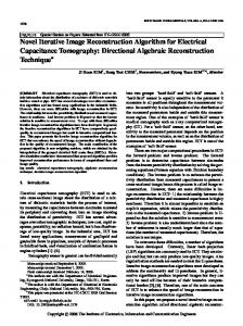
Figure 1. The points of measurement in projection space of a parallel-beam system ( ) (here 11 viewing directions, each with 27 detectors, were chosen), a fan-beam system (×) with five viewing directions with 15 detectors each and the visible light tomography system on RTP (•). For the fan-beam system the origin of each fan is located at three times the reconstruction radius. The p axis has been scaled to the radius a of the reconstruction area.

◦

for a fan-beam system and for the lay-out of the system for visible-light tomography. In section 4 the latter system is described, corrections for beam-width effects are made and the algorithm is applied to actual measurements. The entire discussion in this article assumes the application of the algorithm to two-dimensional emission tomography of an optically thin medium. A discussion of the method in a more general framework of plasma tomography can be found in [4], whereas the visible-light tomography system and measurements have been described in detail in [5, 6]. 2. A description of the algorithm 2.1. Projection space In two-dimensional emission tomography the object under consideration is viewed from several directions in one plane. Each line of sight can be described by two parameters, p and ξ . The impact parameter p is the distance from the line of sight to the origin, namely the centre of reconstruction. The angle ξ is the angle between the line of sight and the x axis. A position in the plane is described by Cartesian coordinates (x, y). The line-integral measurement along the line designated by (p, ξ ) can be written as ZZ f (p, ξ ) = g(x, y)δ(p + x sin ξ − y cos ξ ) dx dy (1) where g(x, y) is the local emissivity of the object and the integral is over the area of the circle with radius a outside which g(x, y) ≡ 0. The parameters p and ξ are coordinates of a space which identifies the line-integral measurements. This space we call projection space. We choose p to be in the range [−a, a] and ξ in the range [0, π ]. The image of the function g(x, y) is called a tomogram, the image of f (p, ξ ) a sinogram. An actual tomography system measures the emission of the object along a finite number of lines and thus 3010

Figure 2. Definitions of the symbols for the bi-linear interpolation between a regular and an irregular grid.

samples the projection space at the same number of points (pi , ξi ), where i counts over the detectors. The coverage of projection space of a multi-view parallel-beam system, a five-view fan-beam system and the visible-light tomography system is shown in figure 1. 2.2. Interpolation method The main function of the reconstruction method in projection space is to relate the values on a regular grid to the signals on an irregular grid by interpolation. The relation between two-dimensional functions determined on the irregular and regular grids is contained in a linear system of equations which describes a bi-linear interpolation from the four regular grid points surrounding each irregular grid point. Following the definition of quantities in figure 2, δp and δξ denoting distances in projection space normalized with respect to the pixel size, one obtains for the weights of interpolation: a1 = (1 − δξ )(1 − δp ) a2 = (1 − δξ )δp a3 = δξ δp

(2)

a4 = δξ (1 − δp ) yielding the relation fi =

4 X

aim fˆm

(3)

m=1

between the measured signals fi and the values fˆm in the surrounding regular grid points m. Equation (3) can be extended to a system of coupled equations including all irregular grid points f = Afˆ (4) where A includes all aim for all detectors i with measurement fi and where m is re-numbered to all regular grid points, with estimated values fˆm . The bi-linear interpolation described in equations (2) and (4) is the simplest interpolation possible, namely only between the closest neighbours. This could be extended in the same

A projection-space reconstruction algorithm

2.3. Step 1: interpolation For iteration l, estimated measurements in the regular grid points m which surround the irregular grid points are obtained by one iteration of the ART inversion method over all l 0 = 1 . . . D detectors. The iterative ART formula is 0 fl 0 − (Afˆl,l −1 )l 0 0 0 fˆml,l = fˆml,l −1 + λl al 0 m kAk2l 0

(5)

P where al 0 m is an element of A, kAk2l 0 = ( i al20 i ), and λl is a relaxation parameter which may be changed during the iterations. At the start of the iteration over l 0 0 0 we assign fˆl,(l =0) ( )fˆl−1 and afterwards fˆl+1 ( )fˆl,(l =D) . The residual norm, needed to estimate the convergence of the iterations, is Rl =

1/2 X [fi − (Afˆl )i ]2 .

(6)

i

2.4. Step 2: smoothing

Figure 3. A schematic representation of the iterative procedure. The symbols and numbering defined in the text are used. The broken box and line are described in section 4.1. If this step is used, f l is calculated and fed back, otherwise only the initial scaled measurement f is used.

scheme to more neighbours, or to, for example, bi-cubic splines, which would make the matrix A more complicated. Simple linear interpolation together with the steps discussed in the next paragraphs proved adequate for our purposes. The underdetermined system of equations (4) is solved iteratively in a way very similar to the algebraic reconstruction technique (ART) in tomographic inversions [7]. The difference with straightforward ART is the application to projection space and the usage of extra steps at each iteration. In each iteration the following steps are taken: step 1, interpolation; step 2, smoothing; step 3, application of boundary conditions; step 4, application of a priori information and constraints; and step 5, tomographic inversion and back-calculation. By back-calculation we mean the re-projection of an estimated emission profile onto the line-integral values that would be measured if the emission profile were the actual one. These back-calculated values we call pseudo-measurements. Some of these steps can be switched off or are not done in all iterations. Each step is discussed below. The main (outer) iteration is designated by iteration number l. All iterative steps described are summarized symbolically in figure 3. The reconstruction steps are preceeded by a scaling of the measurements to correspond to line-integral values (the broken box in figure 3). This will be discussed in section 4.1.

Subsequently smoothing is applied. Apart from smoothing itself, the function of this step is to spread out the interpolation outside the regular grid points that surround measuring points. In principle, smoothing can be included into the matrix A, but here a simpler way was chosen. The smoothing on fˆ is performed by window smoothing, usually in a moving 3 × 3 window; that is, the average over the points in this window is taken as the new value for the central point. Also other types of smoothing have been tried in simulations, such as independent two-dimensional spline smoothing; these gave similar results. 2.5. Step 3: boundary conditions The boundary conditions applied are: fˆ(p, ξ ) = 0

|p/a| ≥ 1

that is, zero emission outside the reconstruction area (radius a) and the periodicity fˆ(p, ξ + π ) = fˆ(−p, ξ ). The latter property is related to the fact that, along a line, the measurement should be the same from either viewing direction. The first boundary condition is obtained by putting the edge values to zero on every iteration. The periodicity is, in principle, already implemented in steps (1) and (2), but could also be imposed by taking the average of the values of fˆ(p, ξ ) at ξ = 0 and ξ = π . 2.6. Step 4: a priori information An initial solution fˆ0 from a priori information about the expected solution or from previously made calculations can be taken into account at the beginning of the iteration. The fˆl can also be modified by forcing them to comply with 3011


constraints such as the conservation of emissivity for each projection: Z a fˆ(p, ξ ) dp = E ∀ξ (7) −a

where E is a constant equal to the total emitted power RR g(x, y) dx dy. Equation (7) is the zeroth moment of fˆ(p, ξ ). Also higher moments can be taken into account in this way. Equation (7) can be applied by scaling the integral over each projection to the average value E of all integrals. For the first moment it is possible to shift the centre of mass of each projection to the line p − r0 sin(θ0 − ξ ) = 0 where r0 and θ0 are the polar coordinates corresponding to the centre of mass of the emission profile. From simulations with phantoms it turned out that application of the conservation-of-emissivity constraint worked well. However, in the case of experimental data more inconsistencies are present than in the numerical simulations and the constraint was not useful to improve the result of reconstructions. 2.7. Step 5: tomographic in version Steps 1–4 achieve the required interpolating and smoothing process in projection space, after which any tomographic inversion method for parallel beams can be used to obtain the corresponding tomogram (step 5a in figure 3). The number of regular grid points after interpolation can be chosen sufficiently large for such methods so that no further assumptions are needed in the tomographic inversion. However, simulations have shown that, if only steps 1– 4 are applied, the resulting sinogram does not yet contain completely consistent data for tomographic inversion. This can be improved by a scheme similar to the Gerchberg– Papoulis iterative scheme between actual space and Fourier space [8]. This Gerchberg–Papoulis-like scheme iterates between projection space and actual space. At this stage of the iteration fˆl is tomographically inverted to result in g l . From this g l the pseudo-measurements along the lines corresponding to the regular grid points in projection space can be back-calculated by equation (1), which replace the previous values fˆl (step 5b in figure 3). These new values are consistent with all properties of projection space and further iterations can make these back-calculated values converge to the measured values. For the tomographic inversion the regularized filtered back-projection (FBP) method described in [9] was used.

3. Results of simulations Simulations with the algorithm described in the previous section were performed on various phantoms, i.e. assumed emission profiles. In this sub-section one phantom has been chosen to illustrate the importance of several parameters for two different systems. Illustrations are given both of the reconstruction in projection space and of subsequent tomographic inversion. In the simulations all dimensions have been normalized with respect to the radius a of the reconstruction region. The phantom was bounded by two circles, one with radius 0.9 and the other with radius 0.5. The larger circle was centred at the centre of the reconstruction, whereas the smaller one was shifted by 0.2 in the x direction. The emission was taken as unity between the circles and zero elsewhere. This phantom simulates the hollow emission profiles that can be expected in certain cases for the visible-light tomography system. Figure 4 gives the phantom and its sinogram. The assumed Gaussian noise had 1% variance, relative to the pseudo-measurement. In step 2 of the algorithm regularized cubic spline smoothing was used both in the p and in the ξ direction. Border values of the sinogram were taken as zero and the conservation of emissivity (equation (7)) was applied. Simulations with the phantom described are discussed in this section, whereas reconstructions of measurements by tomography on the visible-light tomography system are described in section 4. The quality of reconstructions can be judged quantitatively in terms of a number of error measures. In reconstructions of actual measurements only the residual norm of equation (6) is available. In phantom simulations also the relative tomogram error σg =

kg − g0 k kg0 k

(8)

kfˆ − f0 k kf0 k

(9)

and relative sinogram error σfˆ =

can be calculated, where g0 and f0 are the exact tomogram and sinogram values of the phantom. Note the difference between the residual norm and the sinogram error: in the former the difference between the result and the values on the irregular grid is determined, whereas in the latter the difference between the result and the sinogram of the phantom is determined. 3.1. Simulations on a fan-beam system

2.8. Discussion Because all properties of projection space are contained in this method, step 5 automatically implements steps 3 and 4, and also does some smoothing. Because step 5 does not need to be applied on every iteration, implementing steps 3 and 4 can still be useful. The iterations are stopped when the residual norm no longer decreases; that is, when R l+1 ≥ R l , which is a standard breaking criterion for ART methods [10]. 3012

The algorithm was first tested on a fan-beam system with five evenly distributed cameras having 17 detectors each. Such a system has a reasonably uniform coverage of projection space (crosses in figure 1). The relaxation parameter λl was varied. In each simulation it was taken constant, i.e. independent of the iteration l. In figure 5 the tomogram reconstruction error σg is given as a function of iteration l for various λ. Figure 6 shows the tomogram reconstruction error σg , the sinogram reconstruction error


Figure 6. The tomogram reconstruction error, sinogram reconstruction error and residual norm as functions of iteration for a simulation with λ = 2.0 for the fan-beam system. Table 1. Reconstruction error quantities for simulations for 2 ≤ λ ≤ 3. λ

Tomogram error

Sinogram error

Residual norm

2.0 2.1 2.2 2.4 2.5 2.6 3.0

36.1 36.0 35.9 35.8 35.7 48.3 77.1

11.1 11.1 11.0 11.0 11.0 23.5 59.5

4.7 4.6 4.5 4.3 4.8 23.9 47.6

Figure 4. (a) The tomogram and (b) the sinogram of the phantom used in the simulations.

Figure 5. The tomogram reconstruction error σg as a function of iteration l for various relaxation parameters λ for the fan-beam system. The iterations were broken at the point at which the residual norm no longer decreased.

σfˆ and the residual norm for λ = 2.0. It is clear that the convergence of all three quantities is comparable and that the non-decreasing residual is a good criterion for breaking the iteration procedure. Theoretically, the ART as in equation (5) only converges if λ = 0–2 [11, 12]. Here, convergence is found also for λ > 2; the resulting reconstruction-error quantities at the point of breaking of the iterations are given in table 1. The optimum varies for different phantoms. For the above-mentioned phantom it is around λ = 2.4. For larger values the quality of the

reconstruction quickly deteriorates and the reconstruction errors oscillate between iterations (see figure 5). Table 1 shows that the improvement of the optimum λ value over λ = 2 is small; hence λ = 2 or slightly larger is a good choice. Figure 7 shows the reconstructed sinogram and tomogram for λ = 2.0. These results were compared with a different, non-iterative method: a modified version of FBP with a Shepp–Logan filter [13]. The modification consists of bi-linear interpolation of the fan-beam data onto parallel beams and, subsequently, regularized spline smoothing. By the interpolation the desired number of projections and viewing chords can be obtained. It has been found that this method gives reconstructions with the same accuracy as implementations of the exact FBP formula for fan beams, but that it is faster [13]. For comparison the same number of projections and viewing chords as for the interpolation in projection space was used. The result is very similar to figure 7; the reconstruction errors for the tomogram and sinogram (calculated from the reconstructed tomogram) were 37.8 and 11.8%, respectively. This shows that the reconstructions of the new projection-space reconstruction method are of comparable quality to those from the modified FBP method or even slightly better. The main advantage of the new method is that it is applicable to irregularly distributed detection points in projection space, whereas the other method is only suitable for fan-beam systems. 3013


Figure 7. (a) The tomogram and (b) the sinogram of the reconstruction of the phantom with λ = 2.0 for the fan-beam system.

Figure 8. (a) The tomogram and (b) the sinogram of the reconstruction of the phantom with λ = 2.0 for the visible-light tomography system.

3.2. Simulations on the visible-light tomography system

a better fit to the measurements is obtained in projection space, but that the resulting sinogram is not self-consistent. With the Gerchberg–Papoulis-like scheme a self-consistent sinogram is obtained which yields a better tomogram, while the fit of the sinogram to the measured points can be worse. The marginal effect of the Gerchberg-Papoulis-like scheme for fan-beam reconstructions in contrast to the visible-light tomography system can be explained in terms of the more symmetrical coverage of projection space that does not allow inconsistencies by interpolations to appear.

Figure 8 shows the reconstruction of the same phantom for the coverage of projection space of the visible-light tomography system (see figure 1) for λ = 2.0. The reconstruction is reasonably good: the shape of the tomogram, for example the position and the shape of the hole, corresponds well to the phantom. Due to the less uniform coverage and the lack of measurements in some parts the quality of the reconstructions is less than that for the fan-beam system: σg = 43%, σfˆ = 17% and the residual norm is 14%. The convergence of the reconstruction errors for this system is slower than the convergence shown in figure 6 for the fan-beam system: it took approximately 20 iterations to approximate the asymptotic value and the iteration was broken off after 97 iterations. The application of the Gerchberg–Papoulis-like iterations have an important improving effect on the reconstructions for the visible-light tomography system, whereas the effect for the fan-beam system is marginal. For the same parameters as before the omission of the Gerchberg– Papoulis-like scheme results in a better residual norm (10%), but a much worse tomogram reconstruction error (53%) and a less symmetrical tomogram. The reason for this is that, without the Gerchberg–Papoulis-like scheme, 3014

4. Reconstructions of measurements The pseudo-measurements on the regular grid in projection space correspond to pure line integrals according to equation (1), whereas in the actual system effects such as beam width and calibration factors have to be taken into account. The required steps to obtain tomographic reconstructions of measurements by the visible-light tomography system on the RTP tokamak are discussed in this section. 4.1. Description of the visible-light tomography system The 80-channel visible-light tomography system has some properties that make it difficult to apply standard


tomographic reconstruction techniques directly to its measurements. These features include the non-parallelism and the distribution of the relatively few viewing chords, and the width and other properties of the viewing chords. The objectives, design criteria and these properties have been discussed in detail elsewhere [5, 6]. The reconstruction method described in this article was developed to overcome the former difficulty and the nonuniform coverage of projection space. The plasma, which is the light-emitting object under consideration, is viewed from five directions in a plane by 16 detectors each. The positions of the detectors and the viewing directions were largely determined by mechanical constraints. To obtain a sufficient amount of light by sufficiently narrow viewing chords, imaging systems, consisting of spherical mirrors and lenses, relatively close to the plasma are used. Viewing dumps are present to prevent reflections on the walls. The coverage of projection space by the system is given in figure 1. The features of the system can be described by the geometric function W of the system, which describes the contribution of the local emissivity to each detector. For detector i one can write: ZZ Wi (x, y)g(x, y) dx dy. (10) f˜i = The geometrical function contains all information about the system that is needed for tomographic inversion, such as geometrical information and calibration factors. The transformation to a set of parallel beams is not straightforward because the imaging system has properties different from those of lines in parallel-beam systems. The power fi measured along a virtual line with projectionspace coordinates (pi , ξi ), is given by equation (1). The power f˜i measured in reality is given by equation (10). The scaling factor si from measurements of the actual system to ones that would have been measured by pure line-integration is si = fi /f˜i . Note that the scaling factor depends on the emission profile g. For a constant emission profile g(x, y) = 1 inside the plasma and 0 outside, we obtain Li fi = RR Wi (x, y) dx dy f˜i where Li is the chord length through the plasma. The dependence of the scaling factor on g has been studied [5, 14]. For chords viewing the centre of the plasma, the dependence on g is small (< 5%), but for channels viewing the edge the values can be very different for different emission profiles (> 100%). In the reconstructions discussed in this article the scaling factor of a flat profile has been used. For emission profiles with much emission at the edge it may be important to take into account the dependence of the scaling factor on the emission profile, which could be done by including the scaling of the measurements on the basis of the reconstructed g l into the iterations of section 2.

(a)

Figure 9. An example of a tomographic reconstruction of experimental data of the visible-light tomography system on RTP. (a) Contour plot of the reconstructed tomogram. (b) Measurements (•) and back-calculated measurements ( ). In (b) the detectors of the five viewing directions are given consecutively, the tick marks indicating the separation between views.

◦

4.2. Measurements Scaled measurements of continuum emission at the start of a discharge have been reconstructed (figure 9(a)). In this case a peaked symmetrical emission profile is expected, which indeed is obtained from the reconstruction. Backcalculated pseudo-measurements (figure 9(b)) show that, due to the large uncovered parts in projection space, the reconstruction is somewhat oversmoothed. This example demonstrates that physically useful results are obtained by this reconstruction technique and that the scaling process to take into account the optical properties of the system is adequate. More results of measurements have been described elsewhere [5, 15]. 5. Conclusions A new method has been developed to reconstruct projection space, from which tomographic inversions can be performed. For fan-beam systems the method works very well, comparably to other methods. For the visible-light 3015


tomography system on RTP the results of reconstructions both of simulated and of measured data are also good, but, due to the less uniform coverage of projections space, the reconstructions show more smoothing and more artefacts. For the latter system the Gerchberg–Papoulis-like scheme yields a significant improvement of the results. The relaxation parameter for the ART-like iterations for the reconstruction of projection space has been optimized, its optimal value being λ = 2 or slightly larger. The method seems to be a promising new approach to tomographic reconstructions of measurements by systems with irregular coverage and a small number of detectors. Acknowledgments We would like to thank Professors D C Schram and F C Schüller and Dr A J H Donné for their support of our work, and the RTP team for making the measurements possible. This work was performed under the Euratom– FOM association agreement with financial support from the NWO and Euratom. The contribution of V V Pickalov was funded by NWO grant N713-097. References [1] Prince J L and Willsky A S 1990 A geometric projection-space reconstruction algorithm Linear Algebra Appl. 130 151 [2] Prince J L and Willsky A S 1990 Constrained sinogram restoration for limited-angle tomography Opt. Eng. 29 535 [3] Akima H 1978 A method of bivariate interpolation and smooth surface fitting for irregularly distributed data points ACM Trans. Math. Software 4 148

3016

[4] Pickalov V V and Melnikova T S 1995 Plasma Tomography (Novosibirsk: Nauka) (in Russian) [5] Ingesson L C 1995 Visible-light tomography of tokamak plasmas, PhD Thesis, Technische Universiteit Eindhoven, (This thesis can be obtained through the librarian of the FOM-Instituut voor Plasmafysica) [6] Ingesson L C, Koning J J, Donné A J H and Schram D C 1992 Visible light tomography using an optical imaging system Rev. Sci. Instrum. 63 5185 [7] Herman G T 1980 Image Reconstructions from Projections (New York: Academic) [8] Defrise M and De Mol C 1983 A regularized iterative algorithm for limited-angle inverse Radon transform Opt. Acta 30 403 [9] Pickalov V V and Melnikova T S 1984 Tomographic measurements of plasma temperature fields Beitr. Plasmaphys. 24 417 [10] Natterer F 1986 The Mathematics of Computerized Tomography (Stuttgart: Teubner; New York: Wiley) p 89 [11] Herman G T 1980 Image Reconstructions from Projections (New York: Academic) p 184 [12] Natterer F 1986 The Mathematics of Computerized Tomography (Stuttgart: Teubner; New York: Wiley) p 128 [13] Bronnikov A V, Voskobojnikov Yu E, Pickalov V V and Sharapova N V 1988 Comparison of reconstruction algorithms for fan-beam projections Electronnoe Modelirivanie (USSR) 10(6) 81 (in Russian) [14] Ingesson L C, Pickalov V V, Donné A J H and Schram D C 1995 First tomographic reconstructions and a study of interference filters for visible-light tomography on RTP Rev. Sci. Instrum. 66 622 [15] Ingesson L C, Donné A J H, Schram D C and the RTP team 1995 Poloidally asymmetric emission of visible light in RTP Proc. 22nd EPS Conf. on Controlled Fusion and Plasma Physics (Bournemouth) Europhysics Conference Abstracts vol 19C, part VI, ed B E Keen, P E Stott and J Winter (EPS) p 337