An Object-Based Semantic Classification Method for High ... - MDPI

remote sensing Article

An Object-Based Semantic Classification Method for High Resolution Remote Sensing Imagery Using Ontology Haiyan Gu 1, *, Haitao Li 1 , Li Yan 2 , Zhengjun Liu 1 , Thomas Blaschke 3 and Uwe Soergel 4 1 2 3 4

*

Institute of Photogrammetry and Remote Sensing, Chinese Academy of Surveying and Mapping, 28 Lianhuachi Road, Beijing 100830, China; [email protected] (H.L.); [email protected] (Z.L.) School of Geodesy and Geomatics, Wuhan University, Luojiashan, Wuhan 430072, China; [email protected] Department of Geoinformatics—Z_GIS, University of Salzburg, Schillerstrasse 30, Salzburg 5020, Austria; [email protected] Institute for Photogrammetry, University of Stuttgart, Geschwister-Scholl-Str. 24D, 70174 Stuttgart, Germany; [email protected] Correspondence: [email protected]; Tel.: +86-10-6388-0542

Academic Editors: Norman Kerle, Markus Gerke, Sébastien Lefèvre, Xiaofeng Li and Prasad S. Thenkabail Received: 30 December 2016; Accepted: 24 March 2017; Published: 30 March 2017

Abstract: Geographic Object-Based Image Analysis (GEOBIA) techniques have become increasingly popular in remote sensing. GEOBIA has been claimed to represent a paradigm shift in remote sensing interpretation. Still, GEOBIA—similar to other emerging paradigms—lacks formal expressions and objective modelling structures and in particular semantic classification methods using ontologies. This study has put forward an object-based semantic classification method for high resolution satellite imagery using an ontology that aims to fully exploit the advantages of ontology to GEOBIA. A three-step workflow has been introduced: ontology modelling, initial classification based on a data-driven machine learning method, and semantic classification based on knowledge-driven semantic rules. The classification part is based on data-driven machine learning, segmentation, feature selection, sample collection and an initial classification. Then, image objects are re-classified based on the ontological model whereby the semantic relations are expressed in the formal languages OWL and SWRL. The results show that the method with ontology—as compared to the decision tree classification without using the ontology—yielded minor statistical improvements in terms of accuracy for this particular image. However, this framework enhances existing GEOBIA methodologies: ontologies express and organize the whole structure of GEOBIA and allow establishing relations, particularly spatially explicit relations between objects as well as multi-scale/hierarchical relations. Keywords: geographic object-based image analysis; ontology; semantic network model; web ontology language; semantic web rule language; machine learning; semantic rule; land-cover classification

1. Introduction Geographic object-based image analysis (GEOBIA) is devoted to developing automated methods to partition remote sensing (RS) imagery into meaningful image objects, and assessing their characteristics through spatial, spectral, texture and temporal features, thus generating new geographic information in a GIS-ready format [1,2]. There has been great progress compared to traditional per-pixel image analysis. GEOBIA has the advantages of having a high degree of information utilization, strong anti-interference, a high degree of data integration, high classification precision, and less manual editing [3–6]. Over the last decade, advances in GEOBIA research have led to specific algorithms and Remote Sens. 2017, 9, 329; doi:10.3390/rs9040329

www.mdpi.com/journal/remotesensing

Remote Sens. 2017, 9, 329

2 of 21

software packages; peer-reviewed journal papers; six highly successful biennial international GEOBIA conferences; and a growing number of books and university theses [7–9]. A GEOBIA wiki is used to promote international exchange and development [9]. GEOBIA is a hot topic in RS and GIS [1,8] and has been widely applied in global environmental monitoring, agricultural development, natural resource management, and defence and security [10–14]. It has been recognized as a new paradigm in RS and GIS [15]. Ontology originated in Western philosophy and was then introduced into GIS [16]. The concept of domain knowledge is expressed in the form of machine-understandable rulesets and is utilised for semantic modelling, semantic interoperability, knowledge sharing and information retrieval services in the field of GIS [16–18]. Recently, researchers have begun to attach importance to the application of ontology in the field of remote sensing, especially in remote sensing image interpretation. Arvor et al. (2013) described how to utilise ontology experts’ knowledge to improve the automation of image processing and analysis the potential applications of GEOBIA, which can provide theoretical support for remote sensing data discovery, multi-source data integration, image interpretation, workflow management and knowledge sharing [19]. Jesús et al. (2013) built a framework for ocean image classification based on ontologies, which describes how to build ontology model for low and high level of features, classifiers and rule-based expert systems [20]. Dejrriri et al. (2012) presented GEOBIA and data mining techniques for non-planned city residents based on ontology [21]. Kohli et al. (2012) provided a comprehensive framework that includes all potentially relevant indicators that can be used for image-based slum identification [22]. Forestier et al. (2013) built a coastal zone ontology to extract coastal zones using background and semantic knowledge [23]. Kyzirakos et al. (2014) provided wildfire monitoring services by combining satellite images and geospatial data with ontologies [24]. Belgiu et al. (2014a) presented an ontology-based classification method for extracting types of buildings where airborne laser scanning data are employed and obtained effective recognition results [25]. Belgiu et al. (2014b) provided a formal expression tool to express object-based image analysis technology through ontologies [26]. Cui (2013) presented a GEOBIA method based on geo-ontology and relative elevation [27]. Luo (2016) developed an ontology-based framework that was used to extract land cover information while interpreting HRS remote sensing images at the regional level [28]. Durand et al. (2007) proposed a recognition method based on an ontology which has been developed by experts from the particular domain [29]. Bannour et al. (2011) presented an overview and an analysis of the use of semantic hierarchies and ontologies to provide a deeper image understanding and a better image annotation in order to furnish retrieval facilities to users [30]. Andres et al. (2012) demonstrate that expert knowledge explanation via ontologies can improve automation of satellite image exploitation [31]. All these studies focus either on a single thematic aspect based on expert knowledge or on a specific geographic entity. However, existing studies do not provide comprehensive and transferable frameworks for objective modelling in GEOBIA. None of the existing methods allows for a general ontology driven semantic classification method. Therefore, this study develops an object-based semantic classification methodology for high resolution remote sensing imagery using ontology that enables a common understanding of the GEOBIA framework structure for human operators and for software agents. This methodology shall enable reuse and transferability of a general GEOBIA ontology while making GEOBIA assumptions explicit and analysing the GEOBIA knowledge corpus. 2. Methodology The workflow of the object-based semantic classification is organized as follows: in the ontologymodel building step, land-cover models, image object features and classifiers are generated using the procedure described in Section 2.2 (Step 1, Figure 1). The result is a semantic network model. Subsequently, the remote sensing image is classified using a machine learning method and the initial classification result is imported into the semantic network model (Step 2, Figure 1), which is described in Section 2.3. In the last step, the initial classification result is reclassified and validated to get


3 of 21


3 of 20

the final classification result based on the semantic rules (Step 3, Figure 1), which is described in Section The semantic network model is the interactive between the initial classification and Remote Sens. 2017, 9, 329network 3 ofthe 20 the 2.4.2.4. The semantic model is the interactive file file between the initial classification and semantic classification. semantic classification. 2.4. The semantic network model is the interactive file between the initial classification and the Semantic classification Initial classification based semantic classification. Ontology model 1 building for GEOBIA 2 3 based on semantic on Machine learning Ontology model

Create co ncept 1 building fory GEOBIA ontolog Create co ncept ontolog y Build ontology model Land-covers ontology model Build ontology Image object model features ontology model Land-covers Classifier ontology ontology model modelobject Image features ontology model Classifier ontology model Sem antic network

model Sem antic network model

2

Remote sensing based Initial classification imagery learning on Machine Remote sensing Segimagery mentation

Features ontology

Seg mentation Feature selection Features ontology Classifier ontology

Image objects with featues

（OWL format）

Feature selection Initial classification Image objects Classifier ontology

with featues

（OWL format）

Initial class Initial classification information(OWL format) Initial class information(OWL format)

3

Rules Semantic classification Build semantic basedrules on semantic Rules

Classifier ontology Build semantic Features ontology

rules Sem antic classification

Classifier ontology Features ontology

Sem Semantic antic (owl information classification format)

Sem antic OWL transform information(owl format)

to shpfile

Final classification OWL result transform to shpfile

Final classification result

Figure 1. Overview of the methodology followed in this study.

Figure 1. Overview of the methodology followed in this study. Figure 1. Overview of the methodology followed in this study. 2.1. Study Area and Data

2.1. Study Area and Data

The test site is located in Ruili City, in Yunnan Province, China. We utilised panchromatic (Pan) 2.1. Study Area and Data

The located in Ruili City, in 2.1 Yunnan Province, We utilised panchromatic datatest fromsite theis Chinese ZY-3 satellite with m resolution and China. multispectral (MS) ZY-3 data with 5.8(Pan) The test site is located in Ruili City, in Yunnan Province, China. We utilised panchromatic (Pan) m resolution (blue,ZY-3 green, red andwith near-infrared bands), which were acquired(MS) in April 2013. The ZY-5.8 m data from the Chinese satellite 2.1 m resolution and multispectral ZY-3 data with data from the Chinese ZY-3 satellite with 2.1 m resolution and multispectral (MS) ZY-3 data with 5.8 ZY-3 3 MS imagery was obtained and geometricallybands), correctedwhich to the Universal Transverse Mercator resolution (blue, green, red and near-infrared were acquired in April 2013.(UTM) The m resolution (blue, green, red and near-infrared bands), which were acquired in April 2013. The ZYprojection andobtained then re-sampled to 2.1 m to match the Pan image pixel size; it was thenMercator fused using MS imagery was and geometrically corrected to the Universal Transverse (UTM) 3the MSPansharp imagery fusion was obtained and geometrically corrected software. to the Universal Transverse Mercator (UTM) method within the PCI Geomatica Figure 2 shows the resulting fused projection and then re-sampled to 2.1 m to match the Pan image pixel size; it was then fused using the projection and re-sampled to 2.1 m to match image pixel size; it was then fused using image based onthen MS bands 4 (near-infrared), 3 (red)the andPan 2 (green). Pansharp fusion method within the PCI Geomatica software. Figure 2 shows the resulting fused image the Pansharp fusion method within the PCI Geomatica software. Figure 2 shows the resulting fused basedimage on MS bands 4 (near-infrared), 3 (red) and 2 (green). based on MS bands 4 (near-infrared), 3 (red) and 2 (green).

Figure 2. False colour image fusion result of the ZY-3 satellite for Ruili City, China. Figure 2. False colour imagefusion fusion result result of forfor Ruili City, China. Figure 2. False colour image ofthe theZY-3 ZY-3satellite satellite Ruili City, China.


4 of 21

The part of the city selected for the study is characterised by classes identified as Field, Woodland, Grassland, Orchard, Bare land, Road, Building and Water. The eight land-covers are defined based on the Geographical Conditions Census project in China [32], which are described as follows: Field is often cultivated for planting crops, which includes cooked field, new developed field and grass crop rotation land. It is mainly for planting crops, and there are scattered fruit trees, mulberry trees or others. Woodland is covered by natural forest, secondary forest and plantation, which includes trees, bushes, bamboo, etc. Grassland is covered by herbaceous plants, which includes shrub grassland, pastures, sparse grassland, etc. Orchard is artificially cultivated for perennial woody and herbaceous crops. It is mainly used for collecting fruits, leaves, roots, stems, etc. It also includes various trees, bushes, tropical crops and fruit nursery, etc. Bare land is a variety of natural exposed surface (forest coverage is less than 10%). Road is covered by rail and trackless road surface, including railways, highways, urban roads and rural roads. Building includes contiguous building areas and individual buildings in urban and rural areas. Water includes all types of surface water. 2.2. Ontology Model for GEOBIA 2.2.1. Ontology Overview As stated in the introduction section, ontology plays a central part in this methodology. It is used to reduce the semantic gap that exists between the image object domain and the human language centred class formulations of human operators [3,14,19]. The ontology serves as the lynchpin to combine image classification and knowledge formalization. Ontology models are generated for land-cover, image object features, and for classifiers. An ontology is a formal explicit description of concepts and includes: classes (sometimes called concepts), properties of each class/concept describing various features and attributes (slots, sometimes called roles or properties), and restrictions on slots (facets, sometimes called role restrictions). An ontology together with a set of individual instances of classes constitutes a knowledge base [33]. There are many ontology languages, such as Ontology Web Language (OWL), Extensible Markup Language (XML), Description Logic (DL), Resource Description Framework (RDF), Semantic Web Rule Language (SWRL), etc. Ontology building methods include enterprise modelling, skeleton, knowledge engineering, prototype evolution, and so on. There are several ontology building tools, such as ontoEdit, ontolingua, ontoSaurus, WebOnto, OilEd, Protégé, etc., and there are several ontology reasoning machines (Jess, Racer, FaCT++, Pellet, Jena, etc.). In this study, the information for land-cover, object features and machine learning classifiers are expressed in OWL while the semantic rules are expressed in SWRL. The OWL is defined as a recommended standard of ontology language by W3C which is based on the description logic. The relationship of concept and various semantics are expressed by XML/RDF syntax. OWL can describe four kinds of data: class, property, axiom and individual [34]. SWRL is a rule description language which includes OWL-DL, OWL-Lite, RuleML. The knowledge is expressed in OWL by a highly abstract syntax and the combination of Hom-like gauge [35]. The knowledge engineering method and the Protégé software developed by Stanford University have been chosen to build the ontology model for GEOBIA. Our knowledge engineering method consists of seven steps: Step 1 Determine the domain and scope of the ontology. The domain of the ontology is the representation of the whole GEOBIA framework, which includes the information on various features, land-covers and classifiers. We used the GEOBIA ontology to combine land-cover and features for image classification. Step 2 Consider reusing existing ontologies. Reusing existing ontologies may be a requirement if our system needs to interact with other applications that have already been committed to particular ontologies or controlled vocabularies [33]. There are libraries of reusable ontologies on the Web and in the literature. For example, we can use the ISO Metadata [36], OGC [37], SWEET [38], etc. For this study,


Step 3

Step 4

Step 5

Step 6

Step 7

Step 8

5 of 21

we assumed that no relevant ontologies exist a priori and start developing the ontology from scratch. Enumerate important terms in the ontology. We aimed to achieve a comprehensive list of terms, For example, important terms include different types of land-cover, such as PrimarilyVegetatedArea, PrimarilyNonVegetatedArea, and so on. Define the classes and the class hierarchy. There are three main approaches in developing a class hierarchy: top-down, bottom-up, combination. The approach to take depends strongly on the domain [33]. The class hierarchy include land-covers, image object features, classifiers, and so on. Define the properties of classes. The properties become slots attached to classes. A slot should be attached at the most general class that can have that property. For example, image object features should be attached to the respective land-cover. Define the facets of the slots. Slots can have different facets describing the value type, the allowed values, the number of the values (cardinality), and other features of the values the slot can take. For example, the domain of various features is “Region”, the range is “double”. Create instances. Defining an individual instance of a class requires: (1) choosing a class; (2) creating an individual instance of that class; and (3) filling in the slot values [33]. For example, all the segmentation objects are instances, which have their properties. Validation. The FaCT++ reasoner is used to infer the relationship among all the individuals, it could test the correctness and validity of the ontology.

Following this eight-step process, we designed ontology models for GEOBIA, namely for land-cover, image object features, and classifiers. Then, the semantic network model is formed. 2.2.2. Ontology Model of the Land-Cover The Land Cover Classification System (LCCS) includes various land cover classification schemes [39]. In this study, we designed an upper level of classes based on the official Chinese Geographical Conditions Census Project [32] and the upper level of LCCS. The ontology model of the eight land-covers is created as follows. (1) (2)

A list of important terms, including Fields, Woodland, Grassland, Orchards, Bare land, Roads, Building and Water, was created. Classes and class hierarchies were defined. Land cover was defined through the top–down method and was divided into PrimarilyVegetatedArea and PrimarilyNonVegetatedArea. PrimarilyVegetatedArea was divided into ArtificialCropVegetatedArea and NaturalGrowthVegetatedArea. PrimarilyNonVegetatedArea was divided into ArtificialNonVegetatedArea and NaturalNonVegetatedArea. ArtificialCropVegetatedArea is divided into Field and Orchard. NaturalGrowthVegetatedArea is divided into Woodland and Grassland. ArtificialNonVegetatedArea is divided into Building and Road. NaturalNonVegetatedArea is divided into Water and Bare land. The classes are shown in Figure 3. Detailed classes can be defined according to the actual situation.


6 of 21


6 of 20


6 of 20 Owl:Thing Owl:Thing LandCover

PrimarilyVeg etatedArea

LandCover PrimarilyNonVegetatedA rea

PrimarilyVeg etatedArea

PrimarilyNonVegetatedA rea

Artif icial CropVegetatedArea Artif icial CropVegetatedArea

Natural GrowthVegetatedArea Natural GrowthVegetatedArea

Artif icial NonVeg etatedArea Artif icial NonVeg etatedArea

Natural NonVeg etatedArea Natural NonVeg etatedArea

Field

Orchard

Woo dland

Grassland

Building

Road

Water

Bare land

Field

Orchard

Woo dland

Grassland

Building

Road

Water

Bare land

Figure 3. The land-cover ontology (every subclass is shown with an “is.a” relationship).

Figure 3. The land-cover ontology (every subclass is shown with an “is.a” relationship). Figure 3. The land-cover ontology (every subclass is shown with an “is.a” relationship).

2.2.3. Ontology Model of the Image Object Features

2.2.3. Ontology Model of the Image Object Features

2.2.3.Feature Ontology Model is of an theimportant Image Object selection stepFeatures of GEOBIA as there are thousands of potential features Feature selection is an important aslayer there arethousands thousands ofLayerProperty), potential features describing objects. Some of the majorstep categories include:as features (markedofaspotential Feature selection is an important stepof of GEOBIA GEOBIA there are features describing objects. Some of of thethe layer features (marked as LayerProperty), geometry features (marked asmajor GeometryProperty), position features (marked as as PositionProperty), describing objects. Some majorcategories categories include: include: layer features (marked LayerProperty), texture features (marked as class-related features (marked asasClassProperty), and geometry features (marked asTextureProperty), GeometryProperty), position features (marked as PositionProperty), geometry features (marked as GeometryProperty), position features (marked PositionProperty), thematic index (marked as ThematicProperty). The ontology model makes use of the feature concepts texture features (marked TextureProperty),class-related class-related features as ClassProperty), and and texture features (marked as as TextureProperty), features(marked (marked as ClassProperty), used in the eCognition software to develop aThe general upper levelmakes ontology [40]. image object thematic index (marked as ThematicProperty). The ontology model useuse of the feature concepts thematic index (marked as ThematicProperty). ontology model makes ofThe the feature concepts features are through the top–down method and are divided into six categories: LayerProperty, in eCognition the defined eCognition software develop general upper [40]. The image objectobject used used in the software totodevelop aageneral upperlevel levelontology ontology [40]. The image GeometryProperty, PositionProperty, TextureProperty, ClassProperty, and ThematicProperty. Each features are defined through the top–down method and are divided into six categories: LayerProperty, features are defined through the top–down method and are divided into six categories: LayerProperty, feature category can be subdivided further. For instance, the TextureProperty is divided into GeometryProperty, PositionProperty, TextureProperty, ClassProperty, and ThematicProperty. Each GeometryProperty, PositionProperty, TextureProperty, ClassProperty, and ThematicProperty. Each ToParentShapeTexture and Haralick. The Haralick (which stands for Haralick’s texture GLCM feature category can be subdivided further. For instance, the TextureProperty is divided into feature categoryiscan be subdivided further. For instance, the TextureProperty is in divided parameters) divided into GLCMContrast and GLCMEntropy as illustrated Figure into ToParentShapeTexture andGLCMHom, Haralick. The Haralick (which stands for Haralick’s texture GLCM ToParentShapeTexture and Haralick. The Haralick (which stands for Haralick’s texture GLCM 4. parameters) is divided into GLCMHom, GLCMContrast and GLCMEntropy as illustrated in Figure

parameters) is divided into GLCMHom, GLCMContrast and GLCMEntropy as illustrated in Figure 4. 4. Owl:Thing Owl:Thing ObjectProperty

Lay erProperty

GeometryProperty

Lay erProperty

GeometryProperty

Shape

ToGparent

Shape

ToGparent

PositionProperty

ObjectProperty TextureProperty

PositionProperty TextureProperty ToParentSh ToGpolygon apeTexture Haralick ToParentSh ToGpolygon apeTexture Distance Coordinate

ClassProperty

ThematicProperty

ClassProperty ThematicProperty TVeg TSoil TWater TShade TVeg TSoil ToCSub

Haralick ToCNeighbor

TShade

TBuilding

Mean

StdDev

Skewness

ToLPixel

Distance ToLParent Coordinate ToLNeighbor ToLSc ene

ToCNeighbor

SBI

NDMI

NDWI

MNDWI

SI

BAI

NDBI

Mean

StdDev

Skewness

ToLPixel

ToLNeighbor

GLCM Hom

GLCM GLDV GLDV RVI Entropy SBI STDNDVI Contrast

NDMI

NDWI

MNDWI

SI

BAI

NDBI

GLCM Hom

GLCM STD

ToLParent ene GLCM ToLSc GLCM Contrast Entropy GLCM Contrast

GLCM Entropy

ToCSub NDVI RVI

TWater

TBuilding

GLDV Contrast

GLDV Entropy

Figure 4. Image object features ontology (every subclass is shown with an “is.a” relationship). Figure 4. Image object features ontology (every subclass is shown with an “is.a” relationship).

Figure 4. Image object features ontology (every subclass is shown with an “is.a” relationship). 2.2.4. Ontology Model of the Classifiers

2.2.4.Ontology OntologyisModel of theto Classifiers employed express two typical algorithms, namely, decision tree and semantic 2.2.4. Ontology Model of the Classifiers

rules.Ontology is employed to express two typical algorithms, namely, decision tree and semantic

Ontology is employed to express two typical algorithms, namely, decision tree and semantic rules. rules. (1) Ontology model of the decision tree classifier

(1)

(1) The Ontology model of the decision treetree classifier ontology the decision classifier is based on C4.5 algorithm, which is specified Ontology model model of the of decision tree classifier by a set nodes and leaves the nodes Boolean conditions on features andisthe leaves Theofontology model of where the decision tree represent classifier is based on C4.5 algorithm, which specified represent classes.where It is defined as follows. by a set ofland-cover nodes and leaves the nodes represent Boolean conditions on features and the leaves

The ontology model of the decision tree classifier is based on C4.5 algorithm, which is specified represent A land-cover classes.terms, It is defined as follows. of important DecisionTree, Nodeconditions and Leaf, was created. and the leaves by a set of(a) nodeslist and leaves where theincluding nodes represent Boolean on features (b) The slots were defined, which includes relations such as GreaterThan or LessThanOrEqual. A list of classes. important including DecisionTree, Node and Leaf, was created. represent (a) land-cover It terms, is defined as follows. (c) lists of instances of which decision tree, such as Node1, Node2, etc., were The nodes (b) The The slots were defined, includes relations such as GreaterThan or created. LessThanOrEqual.

(a) (c)A are list associated of important terms, including DecisionTree, was created. to features and are also linked to twoNode nodesand with object properties called The lists of instances of decision tree, such as Node1, Node2, etc.,Leaf, were created. The nodes GreaterThan and LessThanOrEqual. (b) The slots were defined, which includes relations such as GreaterThan or LessThanOrEqual. are associated to features and are also linked to two nodes with object properties called GreaterThan and LessThanOrEqual. (c) The lists of instances of decision tree, such as Node1, Node2, etc., were created. The nodes are associated to features and are also linked to two nodes with object properties called GreaterThan and LessThanOrEqual.


7 of 21


7 of 20

The ontology model of of thethe decision is shown shownininFigure Figure The ontology model decisiontree treeclassifier classifier is 5. 5. Owl:Thing is.a


7 of 20

DecisionTree is.a

Root

The ontology model of the decision tree is.a classifier is shown in Figure 5. is.a

Node1 is.a

Node2 is.a is.a Owl:Thing

is.a

is.a Leaf2 Leaf3 DecisionTree

Leaf1

Leaf4

is.a Figure 5. Ontology model of the decision tree classifier.

Figure 5. Ontology model Root of the decision tree classifier. is.a

is.a

(2) Ontology model of the semantic rulesNode1

(2)

Node2

is.a is.a is.a is.a Ontology modelofofmodelling the semantic rules The process semantic rules includes building mark rules and decision rules. Leaf1 Leaf2 Leaf3 Leaf4

Building mark rules is based on a semantic concept, and the process is from low-level features to Figure 5. Ontology model of thebuilding decision tree classifier. The process of modelling semantic includes mark rules decision rules. Building semantic concepts. Decision rules arerules obtained based on mark rules and and a priori knowledge; the is based from advanced featuresconcept, to the identification of land-covers. ontology model of markprocess rules is on a semantic and the process is from The low-level features tomark semantic (2) Ontology model of the semantic rules rules Decision and decision rules shown as follows: concepts. rules areare obtained based on mark rules and a priori knowledge; the process is from The process of modelling semantic rules includes rules and decision rules. advanced(a) features to the identification ofrules land-covers. The building ontologymark model of mark rules and decision Ontology model of the mark Building mark rules is based on a semantic concept, and the process is from low-level features to rules are shown as follows:

The objects are Decision modelledrules fromare different semantic and, according to theknowledge; common sense semantic concepts. obtained basedaspects, on mark rules and a priori the

knowledge, it is advanced divided into: and Planar from the Morphology; Regular and Irregular the (a) Ontology model of theStrip mark rules process is from features to the identification of land-covers. The ontology modelfrom of mark Shape; Smooth andrules Rough the as Texture; Light and Dark from the Brightness; High, Medium and rules and decision arefrom shown follows:

The are modelled from different semantic aspects,from and,the according the common Low objects from the Height; and Adjacent, Disjoint and Containing Position to relationship. Thesense (a) itOntology model of Strip the mark rules knowledge, is divided into: and Planar from the Morphology; Regular and Irregular from ontological model of the mark rules is created as follows. the Shape;The Smooth and Rough from the Texture; Light and Dark from the Brightness; High, Medium objects are modelled from different semantic aspects, and, according to the common sense a) A list of important terms, including Morphology, Shape, Texture, Brightness, Height, and Low from the Disjoint and from the Position relationship. knowledge, it isHeight; dividedand into:Adjacent, Strip and Planar from theContaining Morphology; Regular and Irregular from the The Position, etc., was created. Shape; Smooth and Rough from theisTexture; Light and Dark from the Brightness; High, Medium and ontological model of the mark rules created as follows. b) Class hierarchies were defined. Morphology was divided into Strip and Planar; Shape was Low from the Height; and Adjacent, Disjoint and Containing from the Position relationship. The divided into Regular and Irregular; Texture was divided into Smooth and Rough;

a) A Brightness list of important Morphology, Shape, Texture, Brightness, Height, ontological model of the markterms, rules isincluding created as follows. was divided into Light and Dark; Height was divided into High, Medium and Position, etc., was created. was divided into Adjacent, DisjointShape, and Containing. a) Low; A listand of Position important terms, including Morphology, Texture, Brightness, Height, b) Class hierarchies were defined. Morphology was divided into Strip and Planar; Shape Position, etc., was created. The ontology model of the mark rules is shown in Figure 6. was divided into Regular and Irregular; Texture was divided intoPlanar; Smooth andwas Rough; b) Class hierarchies were defined. Morphology was divided into Strip and Shape Owl:Thin divided into Texture was divided into Smooth andMedium Rough; and Brightness was Regular divided and into Irregular; Light and Dark; Height was divided into High, g Brightness was divided into Light andAdjacent, Dark; Height was divided into High, Medium and Low; and Position was divided into Disjoint and Containing. Position Height and Containing. Texture Brightness Disjoint Morpholo gy Shape Low; and Position was divided into Adjacent,

The ontology model of the mark Figure6.6. The ontology model of the markrules rulesisisshown shown in in Figure Strip

Planar

Smooth

Regular

Hig h

Rough

Owl:Thin Lig ht g

Irregular

Medium

Low

Adjacent

Dark

Disjoint

Containing

Figure 6. The mark rules ontology model (every subclass is shown with an “is.a” relationship). Morpholo gy

Shape

Texture

Brightness

Height

Position

The mark rulesPlanar are expressed in SWRL, and the semantic relationships between the object Hig h Medium Strip Smooth Rough Low features and the classes are built. For example, the Brightness type is expressed in SWRL as follows: Regular

Irregular

Lig ht

Dark

Adjacent

Disjoint

Containing

 Mean (?x, ?y), greaterThanOrEqual (?y, 0.38) -> Light (?x); Figure 6. The ?y), marklessThan rules ontology model (every subclass is shown with an “is.a” relationship).  Mean (?y, 0.38) ->(every Dark (?x). Figure 6. The(?x, mark rules ontology model subclass is shown with an “is.a” relationship). This the Mean feature of an Light, relationships whereas that Light (?x); 

Mean (?x, ?y), lessThan (?y, 0.38) -> Dark (?x).

decision eight types of land-covers are acquired • TheMean (?x,rules ?y), for greaterThanOrEqual (?y, 0.38) -> Lightfrom (?x);literatures, priori knowledge and project technical regulations. Inofgeneral, the decision rules formalized using as follows: This means the Mean feature an object ≥0.38 denotes Light, whereas thatOWL Dark (?x). C(?x), X is an individual of C, P(? X? Y) represents attributes, and x and y are variables.

This means the Mean feature of an object ≥0.38 denotes Light, whereas that Field (?x). The decision rules are expressed in SWRL, and the semantic relationships between the mark This means anthe image object with Regular, Dark, Lowasand adjacentToRoad features rules and classes are built. For example,Planar, the FieldSmooth, is expressed in SWRL follows: Regular (?x), Planar (?x), Smooth (?x), Dark (?x), Low (?x), adjacentToRoad (?x) -> Field (?x). is a Field. This means objectVector with Regular, Planar, Smooth, Dark, LowForest and adjacentToRoad Other classifiers suchanasimage Support Machines (SVM), or Random could be expressed in features is a Field. OWL or SWRL. Later on, the ontology model of the semantic rules can be extended and supplemented Other classifiers such as Support Vector Machines (SVM), or Random Forest could be expressed to realize the semantic understanding variousmodel land-covers. in OWL or SWRL. Later on, theofontology of the semantic rules can be extended and supplemented to realize the semantic understanding of various land-covers.

2.2.5. Semantic Network Model 2.2.5. Semantic Network Model

The entire semantic network model is formed through the construction of the land-covers, image The entire semantic network model is formed through the construction of the land-covers, image object features classifiers usingusing ontology. It Itisisshown inFigure Figure objectand features and classifiers ontology. shown in 7. 7.

Figure 7. The semantic network model. Figure 7. The semantic network model.


9 of 21

The semantic network model is a type of directed network graph that expresses knowledge through the concept and its semantic relations. It has the following advantages. Firstly, the concepts, features, and relationships of geographical entities are expressed explicitly, which could reduce the semantic gap between low-level features and high-level semantics. Second, it can be traced back to the parent object, child objects and neighbourhood objects through their relationships. Third, it is easy to express semantic relations using a computer operable formal language [41]. 2.3. Initial Classification Based on Data-Driven Machine Learning The process includes segmentation, feature selection, sample collection and initial classification. The software FeatureStation developed by the Chinese Academy of Surveying and Mapping is chosen to be the image segmentation and classification tool since it has from its onset on centred around segmentation and decision tree classification. The Protégé plugin developed by Jesús [20] is chosen as the semantic classification tool and for the transformation. 2.3.1. Image Segmentation The objective of image segmentation is to keep the heterogeneity within objects as small as possible, at the same time preserving the integrity of the object. The fusion image is segmented using the G-FNEA method which is based on graph theory and fractal net evolution approach (FNEA) within the FeatureStation software. The method could get high efficiency and maintain good feature boundaries [42]. There are three parameters in the G-FNEA method: T (scale parameter), wcolour (weight factor for colour heterogeneity), and wcompt (weight factor for compactness heterogeneity). A high T value indicates fewer, larger objects than a low T value. The colour heterogeneity wcolour describes the spectral information, which is used to indicate the degree of similarity between two adjacent objects. The higher the wcolour value, the greater influence colour has on the segmentation process. The wcompt value reflects the degree of clustering of the pixels within a region: the lower the value, the more compact the pixels are within the region. It should be noted that the scale parameter is considered to be the most important factor for classification as it controls the relative size of the image objects and has a direct effect on the overall classification accuracy. There are some methods on automatic determination of appropriate segmentation parameters, such as Estimation of Scale Parameters (ESP) [43], Optimised image segmentation [44], SPT (Segmentation Parameter Tuner) [45], Plateau Objective Function [46]. In this study, the selection of image segmentation parameters is based on an iterative trial-and-error approach that is often utilized in object-based classification [6,10]. The best segmentation results were achieved with the following parameters: T = 100, wcolour = 0.8, and wcompt = 0.3. 2.3.2. Feature Selection The selection of appropriate object features can be based on a priori knowledge, or can make use of feature-selection algorithms (such as Random Forest [47]). In this study, we make use of a priori knowledge to guide the initial selection of object features, and thus keep to the following four rules: (1) the most important features of an object are the spectral characteristics, which are independent of test area and segmentation scale; (2) the ratio of bands is closely related to vegetation and non-vegetation; (3) the effect of the shape feature, which is used to reduce the image classification error rate, is small; therefore, it becomes effective when the segmentation scale reaches a certain level, that the objects are consistent with the real surface features; and (4) the auxiliary data (DEM, OpenStreetMap, etc.) is dependent on the scale; the smaller the scale, the more important the auxiliary data. Based on the above four rules, twenty-nine features (e.g., ratio, mean, Normalized Difference Water Index, Normalized Difference Vegetation Index, homogeneity, and brightness) are selected and stored in Shapefile format, and then converted to OWL format. The features of an object in OWL is shown in Figure 8.


10 of 21

Remote Sens. 2017, 9, 329 Remote Sens. 2017, 9, 329

10 of 20 10 of 20

Figure Figure 8. 8. The The features features of of an an object object in in OWL. OWL. Figure 8. The features of an object in OWL.

2.3.3. Initial Classification 2.3.3. Initial Initial Classification Classification 2.3.3. The C4.5 decision tree method is used for the construction of a decision rule, which includes a The C4.5 C4.5 decision decision tree tree method method is is used used for for the the construction of a decision rule, which includes a The generation stage and a pruning stage (Figure 9). construction of a decision rule, which includes a generation stage and a pruning stage (Figure 9). generation stage and a pruning stage (Figure 9).

Training Training samples samples

Sorting Sorting

Computing Computing information information gain rate and gain rate and dividing the dividing trainingthe training samples samples

The decision tree The decisionstage tree generation generation stage

Initial Initialrule decision decision rule

Calculate Calculate expected expected error error probability probability High

Low Low

Cut the Cut the subtree subtree

Final High Keep the Final rule decision Keep the subtree decision rule subtree The decision tree The decision tree prunning stage prunning stage

Figure 9. Decision rule based on C4.5 decision tree classifier. Figure 9. Decision rule based on C4.5 decision tree classifier. Figure 9. Decision rule based on C4.5 decision tree classifier.

(1) (1) (1) (2) (2) (2)

Stage 1: The generation of a decision tree Stage 1: The generation of a decision tree Stagetraining 1: The generation a decision tree The samples areofordered in accordance with the “class, features of sample one, features The training samples are ordered in accordance with features of sample one, features of sample two, etc.” The training and testing samples the are “class, selected by visual image interpretation of sample etc.” The and testing by visual interpretation The training samples aretraining ordered in accordance with are the selected “class, features of image sample one, features with theirtwo, selection being controlled by the samples requirement for precision and representativeness, with their selection being controlled by the requirement for precision and representativeness, of sample two, etc.” The training and testing samples are selected by visual image interpretation and by their statistical properties. and their statistical properties. withby their selection being controlled by the requirement for and precision and representativeness, The training samples are divided. The information gain information gain rate of all and the The training samples are divided. The information gain and information gain rate of all the by their statistical properties. features of training samples are calculated. The feature is taken as the test attribute, whose features of training are calculated. The feature isand as the test attribute, The training samples Theitsinformation gain information gain rate of all information gain ratesamples isare thedivided. biggest and information gain istaken not lower than the mean ofwhose all the the information gain rate is the biggest and its information gain is not lower than the mean of all features of training samples are calculated. The feature is taken as the test attribute, whose features, and the feature is taken as a node and leads to a branch. In this circulation way, all the the features, and the feature is taken as a node and leads to a branch. In this circulation way, all the training samples are divided. training samples are divided.


(3)

11 of 21

information gain rate is the biggest and its information gain is not lower than the mean of all the features, and the feature is taken as a node and leads to a branch. In this circulation way, all the training samples are divided. The generation of decision tree. If all the training samples of the current node belongs to a class, the class is marked as a leaf node and marked for the specify feature. It runs in the same way; Remote Sens. 2017,a9,decision 329 11 of 20 at last, it forms tree until all the data of a subset are recorded in the main feature and their Remote feature value are the same, or there is no feature to divide again. Sens. 2017, 9, 329 11 of 20

(3) The generation of decision tree. If all the training samples of the current node belongs to a class, the is marked as a leaftree. nodeIfand marked for samples the specify feature. It runs inbelongs the same at Theclass generation of decision all the training of the current node toway; a class, Stage(3) 2: The pruning of decision tree.all last, it forms a decision tree node until and the data of subset are feature. recorded theinmain feature and the class is marked as a leaf marked forathe specify It in runs the same way; at their feature are the same, orall there no feature to divide again. in the main feature and last, it formsvalue a decision tree until the is data of a subset are recorded

The possible of sub-node is calculated, the weights of all the nodes theirerror feature value areofthe same, or there not is noleaf-node feature to divide again. Stage 2: Theprobability pruning decision tree. are assessed. The subtree is kept if the error rate causes by cutting off the node is high, otherwise, the Stagepossible 2: The pruning of decisionoftree. The error probability sub-node not leaf-node is calculated, the weights of all the subtree is nodes cut off. last, the decision tree with theerror least expected rate thenode finalis decision tree as areAt assessed. The subtree is kept if the rate causes byerror cutting offisthe high, The possible error probability of sub-node not leaf-node is calculated, the weights of all the shown in Figure 10. The decision tree is expressed in OWL as illustrated in Figure 11. otherwise, the subtree is cut off. At last, the decision tree with the least expected error rate is the final nodes are assessed. The subtree is kept if the error rate causes by cutting off the node is high, decision tree assubtree shown inis Figure 10. last, The into decision is expressed in OWL as illustrated in is Figure 11. classified The above decision ruleis imported thetree semantic network model, allrate objects are otherwise, the cut off. At the decision tree with the least expected error the final The above decision rule is imported into the semantic network model, all objects are classified decision tree as shown in Figure 10.classification The decision treeresult is expressed in OWL asinillustrated in Figure 11. using the decision rule, and the initial is expressed OWL file format. usingThe the above decision rule, and classification result is network expressedmodel, in OWL format. decision rulethe is initial imported into the semantic allfile objects are classified using the decision rule, and the initial classification result is expressed in OWL file format. Landcover Root(node1) NDVI>0.6

Landcover Root(node1)

NDVI>0.6

NDVI0.62 Artificial CropVegetatedArea node4 Artificial CropVegetatedArea

FractalDimension FractalDimension node4 0.37

Natural GrowthVegetatedArea node5 Natural GrowthVegetatedArea Homogeneity Homogeneity >0.71 node5 0.71 Strip (?x); LengthWidthRatio (?x, ?y), lessThan (?y, 1) -> Planar (?x); Homo (?x, ?y), greaterThanOrEqual (?y, 0.05) -> Smooth (?x); Homo (?x, ?y), lessThan (?y, 0.05) -> Rough(?x); Mean (?x, ?y), greaterThanOrEqual (?y, 0.38) -> Light (?x); Mean (?x, ?y), lessThan (?y, 0.38) -> Dark (?x); MeanDEM (?x, ?y), greaterThanOrEqual (?y, 0.6) -> High (?x); MeanDEM (?x, ?y), lessThan (?y, 0.2) -> Low (?x); and MeanDEM (?x, ?y), greaterThanOrEqual (?y, 0.2), lessThan (?y, 0.6) -> Medium (?x).

This means RectFit of an object >0.5 denotes Regular shape, where Field (?x); Irregular (?x), Planar (?x), Rough (?x), Dark (?x), High (?x), adjacentToField (?x)-> Woodland (?x); Regular (?x), Planar (?x), Smooth (?x), Dark (?x), Medium (?x), adjacentToField (?x) -> Orchard (?x); Irregular (?x), Planar (?x), Smooth (?x), Dark (?x), Low (?x), adjacentToBuilding (?x) -> Grassland (?x); Regular (?x), Planar (?x), Rough (?x), Light (?x), High (?x), adjacentToRoad (?x)-> Building (?x); Regular (?x), Strip (?x), Smooth (?x), Light (?x), Low (?x), adjacentToBuilding (?x) -> Road (?x); Irregular (?x), Planar (?x), Rough (?x), Light (?x), Low (?x) -> Bare land (?x); and Irregular (?x), Planar (?x), Smooth (?x), Dark (?x), Low (?x) -> Water (?x).

For example, an object with Regular, Planar, Smooth, Dark and Low features is a Field. C (? X), X is an individual of C, P (? X? Y) represents attributes, and x and y are variables. 2.4.2. Semantic Classification The initial classification result is reclassified and validated to get the final classification result based on the semantic rules. The exported OWL objects are a way to preserve the semantics of the features the image objects exhibits. 3. Results and Discussion 3.1. Results The description, picture, decision tree rules and decision rules of eight land-covers are shown in Table 1.

Table 1. The description, picture, decision tree rules and decision rules of eight land-covers. Description

Picture

Decision Tree Rules

Ontology Rules

Decision Rules in SWRL Format

Table 1. The description, picture, decision tree rules and decision rules of eight land-covers. Field is often cultivated for planting Description


crops, which includes cooked field, new Field is often cultivated for planting

Picture

Decision Tree Rules

Ontology Rules

Decision Rules in SWRL Format

NDVI > 0.6 and

Regular (?x), Planar (?x), Smooth(?x), Dark Table 1. The description, picture,RectangularFit decision tree >rules rules of eight land-covers. developed field and grass crop rotation 0.62 and decision Field ≡ Regular ∩ Planar ∩ Smooth ∩ NDVI > 0.6 and crops, which includes cooked field, new Field (?x),Low(?x), adjacentToRoad(?x) -> Field Description Picture Decision Tree Rules ≤ Rules Decision Rules (?x), in SWRL FormatDark Regular (?x), Planar Smooth(?x), Dark ∩ Ontology Low ∩ adjacentToRoad. land. It is mainly for planting crops, and and FractalDimension developed field and grass crop rotation RectangularFit > 0.62 Field ≡ Regular ∩ Planar ∩ Smooth ∩ (?x) Field often cultivated planting Field (?x),Low(?x), adjacentToRoad(?x) -> Field there is are scattered fruit for trees, mulberry 0.37. Description Picture and FractalDimension Decision Rules Ontology Rules Decision Rules in SWRL Format ∩ Low ∩ adjacentToRoad. land. It is mainly for planting crops, and ≤ TreeDark NDVI > 0.6 and crops, which includes cooked field, new (?x) trees or others. Field is often cultivated for planting crops, Regular (?x), Planar (?x), Smooth(?x), Dark there are scattered fruit trees, mulberry 0.37. field and grass crop rotation RectangularFit > 0.62 Field ≡ Regular ∩ Planar ∩ Smooth ∩ ∩ Planar which includesdeveloped cookedisfield, new developed NDVI > 0.6 and Field ≡ Regular Regular (?x), Planar (?x), Smooth(?x), Orchard artificially cultivated for adjacentToRoad(?x) -> Field others. land. It is mainly fieldField and grass trees croporrotation RectangularFit > 0.62 and ∩ Smooth ∩ Dark ∩ (?x),Low(?x), Low Dark (?x),Low(?x), adjacentToRoad(?x) -> land. It is mainly for crops, and and NDVI FractalDimension Dark ∩ Low ∩ adjacentToRoad. for planting crops, and there scattered fruit ≤ 0.37. ∩ adjacentToRoad. Field (?x) perennial woodyare andplanting herbaceous crops. > FractalDimension 0.6 and ≤ (?x) Orchard is artificially cultivated for trees, mulberry trees or others. Regular (?x), Planar (?x), Smooth(?x), Dark there are scattered fruit trees, mulberry 0.37. > 0.62 RectangularFit Orchard ≡ Regular ∩ Planar ∩ Smooth ∩ It is mainly used for collecting fruits, perennial woody and herbaceous crops. NDVI > 0.6 and Orchard (?x), Medium(?x), adjacentToField(?x) -> trees or roots, others. Orchard is artificially cultivated for Itperennial Regular (?x), Planar (?x), Smooth(?x), Dark leaves, stems, etc. also includes and FractalDimension > Dark ∩ Medium ∩Orchard adjacentToField. ≡ Regular ∩ RectangularFit > 0.62 Orchard ≡ Regular ∩ Planar ∩ Smooth ∩ It is mainlycrops. used for woody and herbaceous It collecting is mainlyfruits, used NDVI > 0.6 and Regular (?x), Orchard (?x)Planar (?x), Smooth(?x), Planar ∩ Smooth ∩ Dark Orchard is artificially forItand (?x), Medium(?x), adjacentToField(?x) RectangularFit > 0.62 and for Orchard collecting fruits, leaves, roots, cultivated stems, etc. Dark (?x), Medium(?x), -> 0.37. various trees, bushes, tropical crops ∩adjacentToField. Medium ∩ leaves, roots, stems, etc. It also includes and FractalDimension > Dark ∩ Medium ∩ FractalDimension > 0.37. also includes various trees, bushes, tropical adjacentToField(?x) -> Orchard (?x) adjacentToField. woody NDVI > 0.6 and Orchard (?x) crops and fruitperennial nursery, etc.etc. and herbaceous crops. fruit nursery, Regular (?x), Planar (?x), Smooth(?x), Dark 0.37. various trees, bushes, tropical crops and RectangularFit > 0.62 Orchard ≡ Regular ∩ Planar ∩ Smooth ∩ It is mainly used for collecting fruits, Woodland is covered of natural forest, NDVI > 0.6 and Woodland ≡ Irregular ∩ Planar ∩ Irregular (?x), Planar (?x), Rough(?x), Dark Orchard (?x), Medium(?x), adjacentToField(?x) -> fruit nursery, etc. Woodland is covered of natural forest, ≡ Irregular ∩ Irregular (?x), Planar (?x), Rough(?x), NDVI > 0.6 leaves, roots, stems, etc. It also includes and FractalDimension > and Dark ∩ Medium ∩Woodland adjacentToField. NDVI > 0.6 and Grassland ≡ Irregular ∩ Planar ∩ Irregular (?x), Planar (?x), Smooth (?x), Grassland is covered of herbaceous Woodlandforest secondary forest and which plantation, which RectangularFit ≤ 0.62 Rough ∩ High (?x), adjacentToField(?x) -> secondary and plantation, includes RectangularFit ≤ 0.62 and∩ Dark Planar ∩ ∩Rough ∩ Dark ∩ High(?x), Dark (?x), High(?x), adjacentToField(?x) Orchard (?x) Woodland is covered of natural forest, NDVI > 0.6 and Woodland ≡ Irregular ∩ Planar ∩ Irregular (?x), Planar (?x), Rough(?x), Dark 0.37. various trees, trees, bushes, bamboo, etc.bushes, tropical crops and Homogeneity > 0.71. High ∩ adjacentToField. -> Woodland (?x) RectangularFit ≤ 0.62 Smooth ∩ Dark ∩ Dark (?x), Low(?x), adjacentToBuilding(?x) Grassland plants, which grassland, includes trees,includes bushes, shrub bamboo, etc. and Homogeneity > 0.71. adjacentToField. Woodland (?x) Woodland secondary forest and plantation, which RectangularFit ≤ 0.62 Rough ∩ Dark ∩ High ∩ (?x), High(?x), adjacentToField(?x) -> fruit nursery, etc. NDVI > 0.6 and Grassland ≡ Irregular ∩ Planar ∩ Irregular (?x), Planar (?x), Smooth (?x), Grassland is covered of herbaceous and Homogeneity ≤ 0.71. Low∩adjacentToBuilding. -> Grassland (?x)Smooth (?x), pastures, grassland, etc. NDVI > 0.6 and Grassland ≡ Irregular ∩ Planar ∩ Irregular (?x), Planar (?x), Grasslandsparse is covered of herbaceous includes trees, bushes,ofbamboo, etc. and Homogeneity > 0.71. adjacentToField. Woodland (?x)Smooth (?x), NDVI > 0.6 and Grassland ≡ Irregular ∩ Planar ∩ Irregular (?x), Planar (?x), Grassland is covered herbaceous RectangularFit ≤ 0.62 Smooth ∩ Dark∩ ∩Planar ∩ Dark (?x),(?x), Low(?x), Grassland plants, which includes grassland, Woodland is covered ofshrub natural forest, NDVI > 0.6 and Woodland ≡ Irregular Irregular PlanaradjacentToBuilding(?x) (?x), Rough(?x), DarkSmooth (?x), Grassland ≡ Irregular ∩ Grassland is covered of herbaceous plants, NDVI > 0.6 and Irregular (?x), Planar (?x), RectangularFit ≤ 0.62 Smooth ∩ Dark ∩ Dark (?x), Low(?x), adjacentToBuilding(?x) Grassland plants, which includes shrub grassland, RectangularFit ≤ 0.62 Smooth Planar ∩ Dark ∩∩ Smooth ∩ Dark Dark ∩ (?x), Low(?x), adjacentToBuilding(?x) Grassland includes shrub grassland, which includes plants, shrub which grassland, pastures, RectangularFit ≤ 0.62 and Dark (?x), Low(?x), and Homogeneity ≤ 0.71. Low∩adjacentToBuilding. -> Grassland (?x) pastures, sparse grassland, etc. sparse Woodland secondary forest and plantation, which RectangularFit ≤ 0.62 Rough ∩ Dark ∩ High ∩ (?x), High(?x), adjacentToField(?x) -> contiguous building NDVI ≤ 0.6 and MeanB1 Regular (?x), Planar (?x),(?x) Rough (?x), and Homogeneity ≤ 0.71. Low∩adjacentToBuilding. -> Grassland pastures,includes sparse grassland, etc. grassland, etc. Building Homogeneity ≤ 0.71. Low∩adjacentToBuilding. adjacentToBuilding(?x) -> Grassland (?x) ≡ Regular ∩ Planar ∩ Rough ∩ and Homogeneity ≤ 0.71. Building Low∩adjacentToBuilding. -> Grassland (?x) pastures, sparse grassland, etc. includes bushes, bamboo,inetc. and Homogeneity adjacentToField. Woodland (?x) Building areas andtrees, individual buildings urban > 0.38 and > 0.71. Light(?x), High(?x), adjacentToRoad (?x) -> Light ∩ High ∩ adjacentToRoad. Building includes contiguous building NDVI ≤ 0.6 and1MeanB1 Regular (?x), Planar (?x), Rough (?x), and rural includes areas. contiguous building LengthWidthRatio ≤ 4.5. Building NDVI ≤ 0.6 and MeanB1 Regular (?x),Building(?x) Planar (?x), Rough (?x), Building ≡ Regular ∩ Planar ∩ Rough ∩ Building includes contiguous building NDVI ≤ 0.6 and MeanB1 (?x), Planar (?x),Planar Rough(?x), (?x), Rough (?x), Building ≡ RegularBuilding ∩ Planar ∩ ≡ Rough ∩ NDVI ≤ 0.6 and MeanB1 Regular ∩ RegularHigh(?x), Regular (?x), Building areas and individual buildings in urban > 0.38 and Light(?x), adjacentToRoad (?x) -> Building includes contiguous building areas and ≡ RegularPlanar ∩ Planar∩∩Rough Rough ∩∩ Light Building areas and individual buildings in urban > 0.38>and Light(?x), adjacentToRoad (?x) -> ∩ High(?x), Light(?x), High(?x), adjacentToRoad (?x) 0.38 1 and Building Light ∩ High ∩ adjacentToRoad. individual in individual urban andbuildings rural areas. Building buildings areas and in urban > 0.38LengthWidthRatio and Light(?x), High(?x), adjacentToRoad (?x) -> Light High ∩ adjacentToRoad. High ∩ adjacentToRoad. Building(?x) ≤∩4.5. and rural areas.by rail and trackless LengthWidthRatio ≤ 4.5. Building(?x) Road is covered NDVI ≤ 0.6 and MeanB1 Regular-> (?x), Strip (?x), Smooth (?x), Light ∩ High ∩ adjacentToRoad. and rural areas. LengthWidthRatio ≤ 4.5. Building(?x) Road ≡ Regular ∩ Strip ∩ Smooth ∩ and rural areas. LengthWidthRatio ≤ 4.5. Building(?x) Road road surface, including railways, > 0.38 and Light(?x), Low(?x), adjacentToBuilding(?x) Light ∩ Low ∩ adjacentToBuilding. Road is covered by rail and trackless NDVI ≤ 0.6 and1MeanB1 Regular (?x), Strip (?x), Smooth (?x), highways, urban by roads rural roads. LengthWidthRatio > 4.5. Road(?x) is covered rail and androad trackless NDVI ≤ 0.6 and MeanB1 Regular (?x),->Strip (?x), Strip Smooth (?x),Smooth (?x), ≡ Regular ∩Road Strip ∩≡Smooth ∩ ∩ Strip Road is coveredRoad by rail and trackless NDVI ≤ 0.6 andRoad MeanB1 Regular ∩ Regular (?x), (?x), Road is covered by rail and trackless NDVI ≤ 0.6 and MeanB1 Regular (?x), Strip (?x), Smooth (?x), Road ≡ Regular ∩ Strip ∩ Smooth ∩ Roadincluding roadrailways, surface, including railways, > 0.38>and Light(?x), adjacentToBuilding(?x) surface, highways, urban 0.38 and Smooth ∩ Light ∩ Low ∩ Low(?x), Light(?x), Low(?x), Road ≡ Regular ∩ Strip ∩ Smooth ∩ Road road surface, including railways, > 0.38 and Light(?x), Low(?x), adjacentToBuilding(?x) Light>∩ 4.5. Low ∩ adjacentToBuilding. roadsRoad and ruralroad roads. LengthWidthRatio adjacentToBuilding.Light(?x), Low(?x), adjacentToBuilding(?x) -> Road(?x) surface, including railways, > 0.38 and adjacentToBuilding(?x) Light ∩ Low ∩ adjacentToBuilding. highways, urban roads and rural roads. LengthWidthRatio > 4.5. -> Road(?x) Light ∩ Low ∩ adjacentToBuilding. highways, urban roads and rural roads. LengthWidthRatio > 4.5. -> Road(?x) highways, urban roads and rural roads. LengthWidthRatio > 4.5. -> Road(?x) Bare land is a variety of natural exposed NDVI ≤ 0.6 and MeanB1 Bare land ≡ Irregular ∩ Planar Rough (?x), Planar (?x), Rough (?x), Bare land∩≡ IrregularIrregular ∩ Bare land is a variety of natural exposed surface NDVI ≤ 0.6 and MeanB1 Irregular (?x), Planar (?x), Rough (?x), Bare land surface (forest coverage is less than Planar ∩ Rough ∩ Light ∩ (forest coverage is less than 10%). Light Low -> Bare land(?x) ≤ 0.38 and NDWI > 0.6. ≤ 0.38 and NDWI > 0.6. ∩ Light Low. ∩ Low. Light (?x), Low(?x), (?x) -> Bare(?x) land(?x) Bare land is a variety of natural exposed 10%). Bare land is a variety of natural exposed NDVI ≤ 0.6 and MeanB1 Bare land ≡ Irregular ∩ Planar ∩ Rough Irregular (?x), Planar (?x), Rough (?x), Bare land is a variety of natural exposed NDVI ≤ 0.6 and MeanB1 Bare land ≡ Irregular ∩ Planar ∩ Rough Irregular (?x), Planar (?x), Rough (?x), Bare land surface (forest coverage is less than NDVI ≤ 0.6 and MeanB1 Bare land ≡ Irregular ∩ Planar ∩ Rough Irregular (?x), Planar (?x), Rough (?x), Bare land surface (forest coverage is less than ≤ 0.38 and NDWI > 0.6. ∩ Light ∩ Low. Light (?x), Low (?x) -> Bare land(?x) Bare land surfaceincludes (forest coverage is less than ≤ 0.38 and NDWI > 0.6. ∩ Light ∩ Low. Light (?x), Low (?x) (?x), -> Bare land(?x) Water all types of surface NDVI ≤ 0.6 and MeanB1 Water ≡ Irregular ∩ Planar ∩ Smooth ∩ Irregular (?x), Planar Smooth (?x), Water ≡ Irregular ∩ 10%). NDVI ≤ 0.6 and MeanB1 Irregular Planar (?x), Smooth (?x), ≤ 0.38 and NDWI > 0.6. ∩ Light ∩ Low. Light (?x), Low (?x)(?x), -> Bare land(?x) Water Water includes10%). all types of surface water. Planar ∩ Smooth ∩ Dark ≤ 0.38 and NDWI ≤ 0.6. Dark (?x), Low (?x) -> 10%). water. ≤ 0.38 and NDWI ≤ 0.6. Dark ∩ Low. Dark (?x), Low (?x) -> Water(?x) Water(?x)

Table 1. The description, picture, decision tree rules and decision rules of eight land-covers.

Field

Orchard

Woodland

Grassland

Building

Road

Bare land

Water

∩ Low.

2

2 2 2

13 of 21


14 of 21

Remote Sens. 2017, 9, x FOR PEER REVIEW

14 of 20

The initial result is expressed in OWL file format defined by the above 14 steps Remote Sens. classification 2017, 9, x FOR PEER REVIEW of 20 of result is expressed in OWL file format defined by the above steps RemoteThe Sens.initial 2017, 9,classification x FOR PEER REVIEW 14 of of 20 segmentation, feature selection, sample collection and initial classification. Figure 12 shows the segmentation, feature selection,result sample collection inand initial classification. Figure showssteps the of The initial is expressed OWL file formatThe defined by the12of above classification ofclassification “region208”, “‘region208’is Water”. expression allsteps the objects’ The result initial classification resultwhereby is expressed in OWL file format defined by the above of classification result of “region208”, whereby “‘region208’is Water”. The expression of all the objects’ segmentation, feature selection, sample collection and initial classification. Figure 12 shows the classification results is the same segmentation, feature selection, sample collection and initial classification. Figure 12 shows the classification results is the sameas as “region208”. “region208”. classification result of “region208”, whereby “‘region208’is Water”. The expression of all the objects’ classification result of “region208”, whereby “‘region208’is Water”. The expression of all the objects’ classification results is the same as “region208”. classification results is the same as “region208”.

Figure Theclassification classification result result of in in OWL. Figure 12.12. The of“region208” “region208” OWL. Figure 12. The classification result of “region208” in OWL.

Figureclassification, 12. The classification resultisofreclassified “region208” in OWL. On the basis of the initial each object and validated by semantic rules in

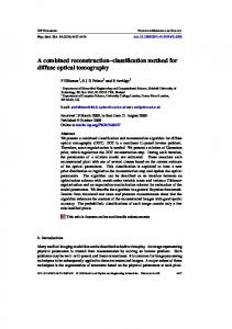
On the basis of the initial classification, each object is reclassified and validated by semantic rules SWRL to obtain the of semantic information. Figure 13 shows a semanticand classification result whererules “the in the basis the initial classification, each object is reclassified validated by semantic in SWRL toOn obtain semantic information. Figure shows a semantic classification result where On the basisthe of the initial classification, each object13 is reclassified and validated by semantic rules in semantic information of ‘region105’ is Regular, Planar, Smooth, Dark, Low, Field”, the expression of SWRL to obtain the semantic information. Figure 13 shows a semantic classification result where all “the “the semantic information of ‘region105’ is Regular, Planar, Smooth, Dark, Low, Field”, theinexpression SWRL to obtain the semantic information. Figure 13 shows semanticobjects classification result where “the thesemantic objects’ classification is the same as “region105”. Thus, theaclassified exported OWL information of ‘region105’ is Regular, Planar, Smooth, Dark, Low, already Field”, the expression of all information of ‘region105’ is Regular, Planar, Smooth, Dark, Field”,objects the expression all of all semantic the objects’ classification isthe the same as “region105”. Thus, the Low, classified alreadyofexported format are help for retrieving object features (Figure 14). the objects’ classification is the same as “region105”. Thus, the classified objects already exported in OWL the objects’ classification isretrieving the same asthe “region105”. Thus, the classified objects already exported in OWL in OWL format are help for object features (Figure 14). format are help for retrieving the object features (Figure 14). format are help for retrieving the object features (Figure 14).

Figure 13. Example of the semantic information in OWL format for “region105”. 13. Example of semantic the semantic informationininOWL OWLformat format for FigureFigure 13. Example of the information for “region105”. “region105”. Figure 13. Example of the semantic information in OWL format for “region105”.

Figure 14. Semantic information of “region105” as displayed in a semantic web interface. Figure 14. Semantic information of “region105” as displayed in a semantic web interface. Figure 14. Semantic information of “region105” as displayed in a semantic web interface.

Figure 14. Semantic information of “region105” as displayed in a semantic web interface.


15 of 20

The semantic classification information in OWL format is transformed to Shapefile format, as shown in Figure 15a. A general object-based decision tree classification without ontology, which Remote Sens. 2017, 9, 329 15 of 21 continues to use “image segmentation, feature extraction, image classification”, was investigated. The segmentation parameters and features are consistent in our method with ontology. The classification Remote Sens. 2017, 9, 329 15 of 20 results aresemantic shown inclassification Figure 15b. information in OWL format is transformed to Shapefile format, The A comprehensive accuracy assessment was carried out. Atree sample-based error matrix is created as shown in Figure 15a. A general object-based decision classification without ontology, The semantic classification information in OWL format is transformed to Shapefile format, as and used for performing accuracy assessment. In GEOBIA, a sample refers to an object. The which continues to use “image segmentation, feature extraction, image classification”, error was shown in Figure 15a. A general object-based decision tree classification without ontology, which matrixes of the two methods forparameters the test areaand are features shown inare Figure 16. The accuracy, producer’s investigated. The segmentation consistent in user’s our method with ontology. continues to use “image segmentation, feature extraction, image classification”, was investigated. The accuracy, overall results accuracy Kappa coefficient The classification areand shown in Figure 15b. are shown in Table 2. segmentation parameters and features are consistent in our method with ontology. The classification results are shown in Figure 15b. A comprehensive accuracy assessment was carried out. A sample-based error matrix is created and used for performing accuracy assessment. In GEOBIA, a sample refers to an object. The error matrixes of the two methods for the test area are shown in Figure 16. The user’s accuracy, producer’s accuracy, overall accuracy and Kappa coefficient are shown in Table 2.

Field

Woodland

Orchard

Road

Grassland

Building

Bare land

Water

(a)

(b)

Figure 15. Land cover classification map from the ZY-3 satellite image for the test site: (a) our method Figure 15. Land cover classification map from the ZY-3 satellite image for the test site: (a) our method with ontology; and (b) decision tree method without ontology. with ontology; and (b) decision tree method without ontology. Field Woodland Orchard Grassland Bare land Field

52.00

2.00

0.00

0.00 Road

0.00

4.00

Building Field

1.00

0.00

2.00 Water

0.00

4.00

0.00

1.00

2.00

0.00

0.00

0.00

0.00

29.00

2.00

3.00

0.00

51.00

A comprehensive accuracy assessment was carried out. A sample-based error matrix is created 0.00 0.00 0.00 Orchard 5.00 57.00 2.00 (a)1.00 0.00 0.00 0.00 0.00 0.00 3.00 2.00 (b) 57.00 Orchard 6.00 and used for performing accuracy assessment. In GEOBIA, a sample refers to an object. The error 0.00 3.00 Woodland 0.00 0.00 0.00 4.00 40.00 0.00 0.00 0.00 1.00 0.00 1.00 41.00 2.00 Woodland 0.00 matrixes the twocover methods for the test in Figure 16.forThe producer’s Figureof15. Land classification maparea fromare the shown ZY-3 satellite image the user’s test site:accuracy, (a) our method Grassland 3.00 1.00 without 3.00 1.00 and 0.00 0.00 2.00 1.00 0.00 36.00 1.00 2. 0.00 Grassland with ontology; (b) 35.00 decision tree3.00 method accuracy, overall accuracy and0.00 Kappa coefficient are ontology. shown 2.00 in Table Building

30.00

2.00

23.00 1.00

3.00 2.00

0.00 0.00

1.00 0.00

47.00 0.00

0.00 0.00

0.00 Bare land 6.00 Orchard

0.00 57.00

0.00 2.00

2.00 3.00

1.00 0.00

2.00 0.00

43.00 0.00

0.00 0.00

Water 0.00 0.00 Woodland

0.00 4.00

0.00 40.00

0.00 0.00

4.00 0.00

0.00 3.00

0.00 0.00

30.00 0.00

4.00 Water 0.00 Woodland

1.00 2.00

0.00 41.00

0.00 1.00

3.00 0.00

0.00 1.00

0.00 0.00

32.00 0.00

Grassland

3.00

1.00

3.00

35.00

0.00

3.00

1.00

0.00

Building

0.00

0.00

0.00

0.00

30.00

2.00

3.00

Road

0.00

0.00

0.00

(a) 0.00

3.00

27.00

2.00

d el Fi

29.00

2.00

3.00

3.00

23.00

3.00

0.00

0.00

0.00

(b) 0.00

1.00

0.00

Building

1.00

0.00

0.00

Road

2.00

1.00

0.00

nd la

2.00

0.00

2.00

nd la

1.00

36.00

Grassland

0.00

er at W

3.00 0.00

3.00 0.00

re Ba

0.00 4.00

1.00 1.00

ad Ro

0.00 0.00

0.00 2.00

g in ild Bu

1.00 2.00

0.00 57.00

1.00

nd la ss ra G d an dl oo W

2.00 Road 51.00 Field

Bare land 5.00 0.00 Orchard

Building

rd ha rc O

0.00 0.00

er at W

2.00 0.00

re Ba

0.00

27.00 1.00

ad Ro

3.00

3.00 0.00

g in ild Bu

0.00 0.00 4.00


0.00 0.00 0.00

rd ha rc O

0.00 0.00 2.00

d el Fi

0.00

Road 52.00 0.00 Field

0.00 0.00

1.00 3.00 0.00 1.00 matrix, 0.00 16. 0.00 47.00 0.00 0.00 43.00 2.00 columns 1.00 2.00objects 0.00 0.00 reference 0.00 land represent Figure Classification confusion where Bare rows and 0.00 method 4.00 0.00(a) our 0.00 0.00 0.00 30.00 and (b) 32.00 0.00 0.00 3.00 ontology. 0.00 0.00 1.00 4.00 Water classified objects: with 0.00 ontology; decision tree method without

Bare land

Water

nd la

er at W

re Ba

ad Ro

g in ild Bu


rd ha rc O

d el Fi

nd la

er at W

re Ba

ad Ro

g in ild Bu


rd ha rc O

d el Fi

(a)

(b)

Figure Figure 16. 16. Classification Classificationconfusion confusionmatrix, matrix,where whererows rowsrepresent representreference referenceobjects objects and and columns columns classified objects: (a) our method with ontology; and (b) decision tree method without ontology. classified objects: (a) our method with ontology; and (b) decision tree method without ontology.


16 of 21

Table 2. Land cover classification accuracy of the two methods. Our Method with Ontology Accuracy

Field Orchard Woodland Grassland Building Road Bare land Water Overall accuracy

Decision Tree Method without Ontology

Production Accuracy (%)

User Accuracy (%)

Production Accuracy (%)

User Accuracy (%)

88.14 87.69 85.11 76.09 85.71 84.38 90.38 88.24

86.67 89.06 88.89 85.37 75 72.97 88.68 100

85.00 83.82 91.11 85.71 82.86 71.88 89.58 80.00

77.27 89.06 95.35 78.26 80.56 76.67 81.13 100

Overall accuracy = 85.95%, Kappa coefficient = 0.84

Overall accuracy = 84.32%, Kappa coefficient = 0.82

The error matrixes (Figure 16, Table 2) reveal that the two methods produce similar results, and only minor differences occur. The overall accuracy of our method with the ontology model is 85.95%, and the kappa coefficient is 0.84. The overall accuracy of the decision tree method without ontology model is 84.32%, and the kappa coefficient is 0.82 (see Table 2). Our method with ontology yields small improvements as it depends on the initial segmentation method. This again is based on the semantic rules used in the semantic classification process which validates the initial classification method furthermore, and some obvious classification errors may be corrected already within the following semantic classification step. The producer’s accuracy of our method for all land-cover types except for Woodland and Grassland are higher than those based on the decision tree method without ontology, as shown in Table 1. The user’s accuracy of our method for Field, Grassland and Bare land are higher than the decision tree method as shown in Table 1. Given that the method employs semantic rules to restrict, it reduces misclassification to a certain extent. However, obvious misclassification instances between Building and Road exist because the two classes are spectrally too similar. 3.2. Discussion The classification results reveal some small improvements of the accuracies when including ontology. However, the ontology model helps in understanding the complex structure of the overall GEOBIA framework, both for the human operators as well as for the software agents used. Even more importantly, the ontology enables the reuse of the general GEOBIA framework, makes GEOBIA assumptions explicit, and enables the operator to analyse the GEOBIA knowledge in great detail. The ontology model of image object features uses the GEOBIA structure as the upper level knowledge to be further extended. The land-cover ontology model is built based on the official Chinese Geographical Conditions Census Project and the upper level of LCCS. It only builds the decision tree ontology model and the semantic rule ontology model, respectively. Both models can be extended to realize the semantic understanding of various land cover categories. The process of image interpretation in the geographic domain—as opposed to, e.g., industrial imaging—is an expert process and many of the parameters need to be tuned depending on the problem domain [19]. We strongly believe that particularly the high degree of variance of natural phenomena in landscapes and potential regional idiosyncrasies can be managed well when formal ontologies serve as a central part the overall GEOBIA framework. The ontology model for land-cover, image object features, and classifiers was formalised through the use of OWL and SWRL formal languages. In fact, the entire semantic network model was built in such a formalized way around the central element of the ontology model for object classification. The knowledge for building the model was acquired both from literature [24] as well as by using data


17 of 21

mining techniques [48,49]. Although the experiments were so far carried out for one high resolution ZY-3 satellite image scene and can therefore not verify the transferability as such, the experiments clearly validated the feasibility of the methodology. The ontology part—as compared to the decision tree classification without using the ontology—yielded only minor statistical improvements in terms of accuracy for this particular image. Still, it validated the ontology to become the central part of a GEOBIA classification framework and a future standard methodology to handle knowledge for a certain domain or for several domains. The authors believe that this methodology can help to reduce the semantic gap which exists in performing image classification [15,19]. Image objects were classified by combining decision tree and semantic rules, which not only provide the classification result of the geographical objects, but also master the semantic information of the geographical entities, and realize the reuse of domain knowledge and the semantic network model. Our results are in line with Arvor et al. [19] who comprehensively portray GEOBIA ontologies for data discovery, automatic image interpretation, data interoperability, workflow management and data publication. In accordance with Blaschke et al. [15], we also want to emphasize the potential to bridge remote sensing and image processing methods with Geoinformatics/GIScience methods. The authors should reemphasize that the methodology is knowledge-driven and shall be shared among experts so as to enhance and share. One obstacle here may be that the software framework used called FeatureStation is very powerful and successfully used in operational studies for the whole of China but it is currently only available in Chinese language and therefore not used internationally. The particular challenges of our method include the determination of an appropriate segmentation scale, the determination of the importance of the various features, the choice of the classifier, and the determination of parameters. Still, all four aspects mentioned are typical to any GEOBIA approach and the ontology provides a great stability for the determination of the parameters and for iterative testing. This study focuses on the implementation process of the method, and overall accuracy is used to evaluate the feasibility of the method. It should be pointed out that the determination of a study of systematic influences of the various elements of the GEOBIA framework on the influence of this method such as the segmentation method, the scale or the features used is simply described in this study, and for the problems and consequences of the different segmentation algorithms, the scale parameter and the feature selection methods we refer to the two recent publications of Ma et al. [50] and Li et al. [51]. 4. Conclusions The study has put forward an object-based semantic classification method for high resolution remote sensing imagery using ontology. It aimed to fully exploit the advantages of ontology to GEOBIA. A detailed workflow has been introduced that includes three major steps: ontology modelling, initial classification based on decision tree machine learning method, and semantic classification based on semantic rules. The structure of the GEOBIA framework was organized organically and expressed explicitly through the ontology. Operationally, the semantic relations were expressed in the OWL and SWRL formal languages with which the software can operate directly. Image objects were classified based on the ontology model by using a decision tree and semantic rules. It could be demonstrated that this ontology based GEOBIA framework can serve as an objective model and can enhance remote sensing image classification, particularly by enhancing the degree of automation and the reusability and transferability of the classification framework. Nevertheless, building a comprehensive ontology is difficult and time-consuming, there is no single correct ontology for any domain, the potential applications of the ontology and the designer’s understanding and view of the domain will undoubtedly affect ontology design choices [33]. Domain experts should be involved in the construction of ontologies. We may also diagnose that, at least in the fields of remote sensing and image classification, ontologies are still rare and have not made their way into standard workflows. As discussed in the introduction section several existing studies have already demonstrated the potential of ontologies for particular domains or specific regional


18 of 21

instances. Our study could clearly go one step further: we created a fully functional comprehensive reusable GEOBIA framework. Further in-depth studies may be required to: (a) improve and refine the GEOBIA ontology model; (b) build ontology models for new classifiers such as deep learning, random forests and random fern; and (c) investigate the automation and “geo-intelligence” potential [52] of the ontology-driven object-based semantic classification method. Particularly through the highly successful GEOBIA conferences such as the 2016 conference organized in Enschede, the Netherlands, worldwide collaborations in ontology research in the field of remote sensing—reaching out to GIS and Geoinformatics—have begun. The authors promote to utilize existing ontologies and the Semantic Web as an extension of the World Wide Web that enables people to share content. It may serve as a web of data and has inspired and engaged scientists to create and share innovative semantic technologies and applications. Therefore, we encourage researchers and experts and to develop shared ontologies to allow for more domain specific ontologies, and to enhance the automation of GEOBIA. Acknowledgments: We thank the anonymous reviewers for their constructive suggestions. This research was funded by: (1) the National Natural Science Foundation of China (Project Nos. 41371406, 41471299, and 41671440); (2) Central Public-interest Scientific Institution Basal Research Fund (Project Nos. 7771508, 777161101, and 777161102); and (3) DAAD-Strategic partnerships and thematic networks 2015–2018, Program line B: Thematic Networks, Stuttgart University (Project No. 57173947). The Protégé software developed by Stanford University was chosen to build the ontology model for GEOBIA. The software FeatureStation developed by the Chinese Academy of Surveying and Mapping was chosen to be the image segmentation and classification tool. The Protégé plugin developed by M. A. J. Jesús was chosen to be the transformation format and semantic classification tool. Norman Kerle’s and Mariana Belgiu’s comments on earlier drafts greatly improved this paper. Author Contributions: This research was mainly performed and prepared by Haiyan Gu and Haitao Li. Haiyan Gu and Haitao Li contributed with ideas, conceived and designed the study. Haiyan Gu wrote the paper. Li Yan and Zhengjun Liu supervised the study and their comments were considered throughout the paper. Thomas Blaschke and Uwe Soergel analysed the results of the experiment, reviewed and edited the manuscript. Conflicts of Interest: The authors declare that they have no conflicts of interest.

References 1.

2.

3.

4. 5.

6.

7. 8. 9.

Hay, G.J.; Castilla, G. Geographic Object-Based Image Analysis (GEOBIA): A New Name for a New Discipline. In Object-Based Image Analysis: Spatial Concepts for Knowledge-Driven Remote Sensing Applications; Blaschke, T., Lang, S., Hay, G.J., Eds.; Springer: New York, NY, USA, 2008; pp. 75–89. Benz, U.C.; Hofmann, P.; Willhauck, G.; Lingenfelder, I.; Heynen, M. Multi- resolution, object-oriented fuzzy analysis of remote sensing data for GIS-ready information. ISPRS J. Photogramm. Remote Sens. 2004, 58, 239–258. [CrossRef] Hay, G.J.; Castilla, G. Object-based image analysis: Strengths, weaknesses, opportunities and threats (SWOT). In Proceedings of the 1st International Conference on Object-Based Image Analysis, Salzburg, Austria, 4–5 July 2006. Robertson, L.D.; King, D.J. Comparison of pixel—And object-based classification in land-cover change mapping. Int. J. Remote Sens. 2011, 32, 1505–1529. [CrossRef] Duro, D.C.; Franklin, S.E.; Dubé, M.G. A comparison of pixel-based and object-based image analysis with selected machine learning algorithms for the classification of agricultural landscapes using SPOT-5 HRG imagery. Remote Sens. Environ. 2012, 118, 259–272. [CrossRef] Myint, S.W.; Gober, P.; Brazel, A.; Grossman-Clarke, S.; Weng, Q. Per-pixel vs. object-based classification of urban land-cover extraction using high spatial resolution imagery. Remote Sens. Environ. 2011, 115, 1145–1161. [CrossRef] Addink, E.A.; Van Coillie, F.M.B.; De Jong, S.M. Introduction to the GEOBIA 2010 special issue: from pixels to geographic objects in remote sensing image analysis. Int. J. Appl. Earth Obs. 2012, 15, 1–6. [CrossRef] Blaschke, T. Object based image analysis for remote sensing. ISPRS J. Photogramm. Remote Sens. 2010, 65, 2–16. [CrossRef] GEO-Object-Based Image Analysis. Available online: http://wiki.ucalgary.ca/page/GEOBIA (accessed on 5 May 2016).


10. 11. 12. 13. 14.

15.

16. 17. 18. 19.

20. 21.

22. 23. 24.

25. 26. 27. 28. 29.

30.

19 of 21

Pu, R.; Landry, S.; Yu, Q. Object-based urban detailed land-cover classification with high spatial resolution IKONOS imagery. Int. J. Remote Sens. 2011, 32, 3285–3308. [CrossRef] Hussain, M.; Chen, D.M.; Cheng, A.; Wei, H.; Stanley, D. Change detection from remotely sensed images: From pixel-based to object-based approaches. ISPRS J. Photogramm. Remote Sens. 2013, 80, 91–106. [CrossRef] Blaschke, T.; Hay, G.J.; Weng, Q.; Resch, B. Collective sensing: integrating geospatial technologies to understand urban systems—An overview. Remote Sens. 2011, 3, 1743–1776. [CrossRef] Nussbaum, S.; Menz, G. Object-Based Image Analysis and Treaty Verification: New Approaches in Remote Sensing-Applied to Nuclear Facilities in Iran; Springer: New York, NY, USA, 2008. Lang, S. Object-based image analysis for remote sensing applications: Modeling reality-dealing with complexity. In Object-Based Image Analysis: Spatial Concepts for Knowledge-Driven Remote Sensing Applications; Blaschke, T., Lang, S., Hay, G.J., Eds.; Springer: New York, NY, USA, 2008; pp. 3–27. Blaschke, T.; Hay, G.J.; Kelly, M.; Lang, S.; Hofmann, P.; Addink, E.; Feitosa, R.; van der Meer, F.; van der Werff, H.; Van Coillie, F.; et al. Geographic Object-based Image Analysis: A new paradigm in Remote Sensing and Geographic Information Science. ISPRS J. Photogramm. Remote Sens. 2014, 87, 180–191. [CrossRef] [PubMed] Agarwal, P. Ontological considerations in GIScience. Int. J. Geogr. Inf. Sci. 2005, 19, 501–536. [CrossRef] Li, J.L.; He, Z.Y.; Ke, D.L.; Zhu, Q.L.A. Approach for Insight into Geo-ontology Merging based on Description Logics. Geomat. Inf. Sci. Wuhan Univ. 2014, 39, 317–321. Li, Q.C. Research of Model and Methods Based on Ontology for Geo-Information Semantic Transformation. Ph.D. Thesis, PLA Information Engineering University, ZhengZhou, China, 2011. Arvor, D.; Durieux, L.; Andres, S.; Laporte, M.A. Advances in Geographic Object-Based Image Analysis with ontologies: A review of main contributions and limitations from a remote sensing perspective. ISPRS J. Photogramm. Remote Sens. 2013, 82, 125–137. [CrossRef] Jesús, M.A.J.; Luis, D.; José, A.P.F. A Framework for Ocean Satellite Image Classification Based on Ontologies. IEEE J. Sel. Top. Appl. Earth Obs. Remote Sen. 2013, 6, 1048–1063. Dejrriri, K.; Malki, M. Object-based image analysis and data mining for building ontology of informal urban settlements. In Proceedings of the SPIE Image and Signal Processing for Remote Sensing XVIII, Edinburgh, UK, 24 September 2012. Kohli, D.; Sliuzas, R.; Kerle, N.; Stein, A. An ontology of slums for image-based classification. Comput. Environ. Urban Syst. 2012, 36, 154–163. [CrossRef] Forestier, G.; Puissant, A.; Wemmert, C.; Gançarski, P. Knowledge-based region labeling for remote sensing image interpretation. Comput. Environ. Urban Syst. 2012, 36, 470–480. [CrossRef] Kyzirakos, K.; Karpathiotakis, M.; Garbis, G.; Nikolaou, C.; Bereta, K.; Papoutsis, I.; Herekakis, T.; Michail, D.; Koubarakis, M.; Kontoes, C. Wildfire monitoring using satellite images, ontologies and linked geospatial data. Web Semant. 2014, 24, 18–26. [CrossRef] Belgiu, M.; Tomljenovic, I.; Lampoltshammer, T.J.; Blaschke, T.; Höfle, B. Ontology-based classification of building types detected from airborne laser scanning data. Remote Sens. 2014, 6, 1347–1366. [CrossRef] Belgiu, M.; Höfle, B.; Hofmann, P. Coupling formalized knowledge bases with object-based image Analysis. Remote Sens. Lett. 2014, 5, 530–538. [CrossRef] Cui, W.; Tang, S.; Li, R.; Yao, Z. A method of Identifying Remote Sensing Objects by using Geo-ontology and Relative Elevation. J. Wuhan Univ. Technol. 2013, 37, 695–698. Luo, H.; Li, L.; Zhu, H.; Kuai, X.; Zhang, Z.; Liu, Y. Land Cover Extraction from High Resolution ZY-3 Satellite Imagery Using Ontology-Based Method. ISPRS Int. J. Geo-Inf. 2016, 5, 31. [CrossRef] Durand, N.; Derivaux, S.; Forestier, G.; Wemmert, C.; Gancarski, P.; Boussaid, O.; Puissant, A. Ontology-Based Object Recognition for Remote Sensing Image Interpretation. In Proceedings of the IEEE International Conference on TOOLS with Artificial Intelligence, Patras, Greece, 29–31 October 2007; pp. 472–479. Bannour, H.; Hudelot, C. Towards ontologies for image interpretation and annotation. In Proceedings of the International Workshop on Content-Based Multimedia Indexing, Madrid, Spain, 13–15 June 2011; pp. 211–216.


31.

32. 33. 34. 35. 36.

37.

38.

39. 40. 41. 42.

43. 44. 45.

46.

47. 48. 49.

50.

20 of 21

Andres, S.; Arvor, D.; Pierkot, C. Towards an ontological approach for classifying remote sensing images. In Proceedings of the Eighth International Conference on Signal Image Technology and Internet Based Systems, Naples, Italy, 25–29 November 2012; pp. 825–832. Geographical Conditions Census Contents and Index (GDPJ 01—2013). Available online: http://www.jschj. gov.cn/upfile/dlgqdoc/jswd/GDPJ012013.pdf (accessed on 5 February 2016). Ontology Development 101: A Guide to Creating Your First Ontology. Available online: http://protege. stanford.edu/publications/ontology_development/ontology101.pdf (accessed on 5 February 2016). OWL Web Ontology Language Reference. Available online: http://www.w3.org/TR/owl-ref/ (accessed on 5 February 2016). SWRL: A Semantic Web Rule Language Combining owl and RuleML. Available online: http://www.w3. org/Submission/SWRL/ (accessed on 5 February 2016). ISO-Metadata.owl: Several ISO Geographic Information Ontologies developed with the Protege-OWL editor. Contributed by Akm Saiful Islam, Bora Beran, Luis Bermudez, Stephane Fellah & Michael Piasecki. Available online: http://protegewiki.stanford.edu/wiki/Protege_Ontology_Library (accessed on 5 February 2016). OGC: Ontology for Geography Markup Language (GML3.0) of Open GIS Consortium (OGC). Contributed by Contributors: Zafer Defne, Akm Saiful Islam and Michael Piasecki. Available online: http://protegewiki. stanford.edu/wiki/Protege_Ontology_Library (accessed on 5 February 2016). SWEET Ontologies: A Semantic Web for Earth and Environmental Terminology. Source: Jet Propulsion Laboratory. Available online: http://protegewiki.stanford.edu/wiki/Protege_Ontology_Library (accessed on 5 February 2016). Di Gregorio, A. Land Cover Classification System: Classification Concepts and User Manual: LCCS; Food and Agriculture Organization: Rome, Italy, 2005. Definiens Imaging GmbH. Developer 8 Reference Book; Definiens Imaging GmbH: Munich, Germany, 2011. Tonjes, R.; Glowe, S.; Buckner, J.; Liedtke, C.E. Knowledge-based interpretation of Remote Sensing images using semantic nets. Photogramm. Eng. Rem. S. 1999, 65, 811–821. Yang, Y.; Li, H.T.; Han, Y.S.; Gu, H.Y. High resolution remote sensing image segmentation based on graph theory and fractal net evolution approach. In Proceedings of the International Workshop on Image and Data Fusion, Kona, HI, USA, 21–23 July 2015. Drˇagu¸t, L.; Tiede, D.; Levick, S.R. ESP: A tool to estimate scale parameter for multiresolution image segmentation of remotely sensed data. Int. J. Geogr. Inf. Sci. 2010, 24, 859–871. [CrossRef] Gao, Y.; Mas, J.F.; Kerle, N.; Navarrete Pacheco, J.A. Optimal region growing segmentation and its effect on classification accuracy. Int. J. Remote Sens. 2011, 32, 3747–3763. [CrossRef] Achanccaray, P.; Ayma, V.A.; Jimenez, L.I.; Bernabe, S. SPT 3.1: A free software tool for automatic tuning of segmentation parameters in optical, hyperspectral and SAR images. In Proceedings of the IEEE International Geoscience and Remote Sensing Symposium, Milan, Italy, 26–31 July 2015. Martha, T.R.; Kerle, N.; van Westen, C.J.; Jetten, V.; Kumar, K.V. Segment Optimization and Data-Driven Thresholding for Knowledge-Based Landslide Detection by Object-Based Image Analysis. IEEE Trans. Geosci. Remote. 2011, 49, 4928–4943. [CrossRef] Stumpf, A.; Kerle, N. Object-oriented mapping of landslides using Random Forests. Remote Sens. Environ. 2011, 115, 2564–2577. [CrossRef] Maillot, N.; Thonnat, M.; Boucher, A. Towards ontology-based cognitive vision. Mach. Vis. Appl. 2004, 16, 33–40. [CrossRef] Belgiu, M.; Drˇagu¸t, L.; Strobl, J. Quantitative evaluation of variations in rule-based classifications of land cover in urban neighbourhoods using WorldView-2 imagery. ISPRS J. Photogramm. Remote Sens. 2014, 87, 205–215. [CrossRef] [PubMed] Ma, L.; Li, M.; Blaschke, T.; Ma, X.; Tiede, D.; Cheng, L.; Chen, Z.; Chen, D. Object-based change detection in urban areas: the effects of segmentation strategy, scale, and feature space on unsupervised methods. Remote Sens. 2016, 8, 761–778. [CrossRef]


51.

52.

21 of 21

Li, M.; Ma, L.; Blaschke, T.; Cheng, L.; Tiede, D. A Systematic Comparison of Different Object-Based Classification Techniques Using High Spatial Resolution Imagery in Agricultural Environments. Int. J. Appl. Earth Obs. 2016, 4, 87–98. [CrossRef] Hofmann, P.; Lettmayer, P.; Blaschke, T.; Belgiu, M.; Wegenkittl, S.; Graf, R.; Lampoltshammer, T.J.; Andrejchenko, V. Towards a framework for agent-based image analysis of remote-sensing data. Int. J. Image Data Fusion 2015, 6, 115–137. [CrossRef] [PubMed] © 2017 by the authors. Licensee MDPI, Basel, Switzerland. This article is an open access article distributed under the terms and conditions of the Creative Commons Attribution (CC BY) license (http://creativecommons.org/licenses/by/4.0/).

An Object-Based Semantic Classification Method for High ... - MDPI

An Object-Based Semantic Classification Method for High ... - MDPI

Suggest Documents

Pixel-Wise Classification Method for High Resolution Remote ... - MDPI

An SVM-Based Method for Classification of External ... - MDPI

An Ensemble Method for Multilabel Classification - Semantic Scholar

An Extension of the Classification-Tree Method for ... - Semantic Scholar

Fuzzy Classification Method for Processing ... - Semantic Scholar

An Automated Method for High-Definition ... - Semantic Scholar

Automatic Crack Detection and Classification Method for ... - MDPI

A Method for Load Classification and Energy Scheduling ... - MDPI

Automatic Crack Detection and Classification Method for ... - MDPI

Automatic Crack Detection and Classification Method for ... - MDPI

Supervised Classification High-Resolution Remote-Sensing ... - MDPI

an efficient automatic mass classification method ... - Semantic Scholar

An ICA-based Gene Classification/Clustering Method

Texture Classification Method using Wavelet ... - Semantic Scholar

An improved DNA array-based classification method for the ... - Plos

An Effective Method for Imbalanced Time Series Classification: Hybrid

An unsupervised classification method for inferring original case ...

Remote Sensing Image Classification Method ... - Semantic Scholar

A combined reconstruction--classification method ... - Semantic Scholar

An Efficient Method for Extracting Fuzzy Classification ... - CiteSeerX

An Optimal Classification Method for Biological and Medical Data

An Effective Classification Method for Facebook Data - DergiPark

Micro-Blog Emotion Classification Method ... - Semantic Scholar

Development of an experimental classification method for second life ...