Learning to trade with incremental support vector regression experts. Giovanni Montana and Francesco Parrella. Department of Mathematics. Imperial College ...
Learning to trade with incremental support vector regression experts Giovanni Montana and Francesco Parrella Department of Mathematics Imperial College London
Abstract. Support vector regression (SVR) is an established non-linear regression technique that has been successfully applied to a variety of predictive problems arising in computational finance, such as forecasting asset returns and volatilities. In real-time applications with streaming data two major issues that need particular care are the inefficiency of batch-mode learning, and the arduous task of training the learning machine in presence of non-stationary behavior. We tackle these issues in the context of algorithmic trading, where sequential decisions need to be made quickly as new data points arrive, and where the data generating process may change continuously with time. We propose a master algorithm that evolves a pool of on-line SVR experts and learns to trade by dynamically weighting the experts’ opinions. We report on risk-adjusted returns generated by the hybrid algorithm for two large exchange-traded funds, the iShare S&P 500 and Don Jones EuroStoxx 50.
Key words: Incremental support vector regression, subspace tracking, ensemble learning, computational finance, algorithmic trading
1
Introduction
Support vector regressions (SVRs) are state-of-art learning machines for solving linear and non-linear regression problems. Over the last few years, SVRs have been successfully applied to a number of different tasks in computational finance, most notably the prediction of future price movements and asset returns. A variety of SVR architectures have been proposed with applications to different asset classes including equities [19, 1] and foreign exchange rates [3, 12]. In some cases, hybrid approaches combine standard econometric forecasting models with more flexible SVR algorithms that are able to capture potential non-linear patterns in historical data [10]. Other than expected returns, some initial work has also been done towards forecasting the volatility of an asset [6, 9] as well as the its direction of change [11]. A major difficulty in dealing with financial time series representing asset prices is their non-stationary behavior (or concept drift), i.e. the fact that the underlying data generating mechanism keeps changing over time. Some adaptive SVR algorithms have been proposed [23], where more recent errors are penalized
2
Giovanni Montana and Francesco Parrella
more heavily by appropriately modifying the ǫ-insensitive loss function. However, these approaches are based on algorithms that learn from the data in batch-mode, so that when new data points are made available, the learning machine has to be retrained again. Batch learning can be highly inefficient and can introduce costly delays in the decision making process, particularly so in time-aware applications such as algorithmic trading where the data streams used as inputs by the learning machine may be imported at very high sampling frequencies (e.g. every minute or less). In real-time forecasting and trading applications one is often interested in on-line learning, a situation where the regression function is updated following the arrival of each new sample. Various approaches for incremental learning with support vector machines have been proposed in the literature, for both classification [4, 13, 27] and regression problems [15, 26, 16]. In this paper we propose an hybrid learning algorithm in the context of algorithmic equity trading. The algorithm decides how many shares of a given security to buy or short sell at any given point in time. Short selling is the practice of borrowing a security for an immediate sale, with the understanding that it will be bought back later. By using short selling, the trading machine can benefit from decreases, not just increases, in the prices, and could achieve financial returns that are only mildly correlated with the market returns. This class of strategies is often referred to as market neutral or relative value [20]. At the core of our approach there is an on-line SVR algorithm that learns the relationship between the observed security price and the underlying market conditions, and then suggests in real-time whether the security being traded is currently underpriced or overpriced, relative to the market. The market conditions are represented by patterns, in the form of latent factors, that are dynamically extracted from a (possibly very large) collection of cross-sectionally observed financial data streams. Section 2 contains a concise description of our on-line SVR algorithm. In practice, the assumed relationship between the marker factors and the target security constantly evolves over the time, and failing to capture these changes can crucially affect the performance of the trading algorithm. We propose an ensemble learning approach. Our solution consists in evolving an ensemble of SVR experts, where each expert is characterized by a specific set of hyperparameters. A master algorithm, detailed in Section 3, is then responsible for weighting these expert opinions and taking a final trading decision. In Section 4, the meta algorithm is empirically shown to outperform the best SVR expert in the ensemble in terms of risk-adjusted returns.
2
Asset pricing with incremental SVR
In this section we describe how SVR is applied to price a security purely on the basis on market data, in an incremental fashion. Suppose that, on each trading day i, the security price is denoted by yi , and we have made t observations. We envisage a situation where n cross-sectional financial data streams representative of the target market are observed and collected, at each discrete time, in a
Learning to trade with incremental support vector regression experts
3
vector si . Since n may be very large, we sequentially project the data onto the directions of maximal variability in order to extract an input vector or pattern xi of dimension k < n (see also Section 3). With the most updated input vector xt at hand, we then wish to obtain an updated estimate of yt , say yˆt . In our approach, this estimate is obtained as f (xt ) = wφ(xt ) + b, where w is a weight vector, φ(·) is a non-linear mapping from input space to some high-dimensional feature space, and b is a scalar representing the bias. In order to perform the estimation task above, we adopt the SVR framework based on the ǫ-insensitive loss function [24]. Accordingly, we are willing to accept that price estimates that are within ±ǫ of the observed price yt are always considered fair prices, for a given positive scalar ǫ. Estimation errors less than ǫ are ignored, whereas errors larger than ǫ result in additional linear losses [7]. Introducing slack variables ξi , ξi∗ quantifying estimation errors greater than ǫ, the price estimation task can be formulated as a constrained optimization problem: we search for w and b that minimize the regularized loss X 1 T (ξi + ξi∗ ) w w+C 2 i=1 t
(1)
subject to constraints −yi + (wT φ(xi ) + b) + ǫ + ξi ≥ 0, yi − (wT φ(xi ) + b) + ǫ + ξi∗ ≥ 0 and ξi , ξi∗ ≥ 0 for all i = 1, . . . , t, where a penalization on the norm of the weights has been imposed and is controlled by the parameter C. As it is commonly done, we transform this primal optimization problem to its dual quadratic optimization problem. The Representer Theorem [25] assures us that the solution to the resulting optimization problem may be expressed as f (x) =
t X
θi K(xi , x)
(2)
i=1
where θi is defined in terms of the dual variables and K(·, ·) is a kernel function [22]. In our application, we adopt a Gaussian kernel depending upon the specification of a hyperparameter σ. Our objective is to minimize (1) incrementally, without having to retrain the model entirely at each time point. Following [4, 15], an incremental version of SVR can be obtained by first classifying all training points into three distinct auxiliary sets according to the KKT conditions that define the current optimal solution. Specifically, after defining the margin function hi (xi ) as the difference f (xi ) − yi for all time points i = 1, . . . , t, the KKT conditions can be expressed in terms of θi , hi (xi ), ǫ and C. Accordingly, each data point falls into one of the following sets, S = {i | (θi ∈ [0, +C] ∧ hi (xi ) = −ǫ) ∨ (θi ∈ [−C, 0] ∧ hi (xi ) = +ǫ)} E = {i | (θi = −C ∧ hi (xi ) ≥ +ǫ) ∨ (θi = +C ∧ hi (xi ) ≤ −ǫ)}
(3)
R = {i | θi = 0 ∧ |hi (xi )| ≤ ǫ} Set S contains the support vectors, i.e. the data points contributing to the current solution, whereas the points that do not contribute are contained in
4
Giovanni Montana and Francesco Parrella
R. All other points are in E. When a new data point arrives, the incremental algorithm relabels all points in an iterative way till optimality is reached again. Similarly, old data points can be discarded easily without having to retrain the machine. Our specific implementation mostly differs from [15] in the definition of the auxiliary sets (3). Full details can be found in [21].
3
Learning to trade with expert advice
Let us suppose that we were able to select the hyperparameter triple (ǫ, C, σ) yielding a regression function f (xt ) of form (2) that truly describes the relationship between the current market patterns xt and the fair price of the target security. Based on historical data up to date, this regression model would produce an estimate yˆt of the fair price, and a corresponding estimate m ˆ t = yt − yˆt of the discrepancy between observed and estimated price. We can now make the following observations. If the above relationship was not affected by noise, and if markets were always perfectly efficient, we would have that m ˆ t = 0 at all times. On the other hand, when |m ˆ t | > 0, an arbitrage opportunity arises. For instance, a negative m ˆ t would indicate that the security is under-valued, and a sensible decision would be to buy shares of the security, compatibly with the expectation that the markets will promptly react to this temporary inefficiency by moving the price up. Analogously, a positive m ˆ t would suggest to short sell a number of shares in accordance with the expectation that the price will be decreasing over the following time interval. Further insights and explanations regarding this relative value trading strategy can be found in [8, 2, 18]. In a realistic setting, tuning the hyperparameter triple is an arduous task. Moreover, an optimal choice may soon become sub-optimal, due to the highly dynamic nature of the data under consideration. For this reason, we have chosen to pursue an hybrid approach consisting of a collection of SVR experts. On each trading day, a master algorithm adopting the weighted majority voting principle [14] collects the opinion of E experts, each one suggesting whether to buy or short sell the security, and takes a final decision. In summary, the following operations are performed at any given time t, after observing the most recent data pair (st , yt ): Pattern extraction: A pattern xt is extracted from the data stream vector st by projecting st onto the eigenvector corresponding to the largest eigenvalue. An estimate of the eigenvector at time t, denoted ht , is given by a recursive updating equation, ˆ ˆ t−1 + 1 st sT ht−1 ˆt = t − 1 h h t ˆ t t ||ht−1 || Note how this solution does not require the explicit computation of the covariance matrix (see [28] for derivations). Expert opinion: Each expert in the pool produces a mispricing estimate (e)
m ˆt
(e)
= yt − yˆt
e = 1, . . . , E
(4)
Learning to trade with incremental support vector regression experts
5
0.01
2500
0.001 2000
ε
Expert Index
0.0001 1500 1e−05
1000 1e−06
500
1e−07
6
12
18
24 30 Month
36
42
48
1e−08 1000
1010
1020
1030
1040
1050 Day
1060
1070
1080
1090
1100
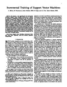
Fig. 1. DJ EuroStoxx 50: time-dependence of the best expert (left) and timedependence of the ǫ hyperparameter corresponding to the best expert for a few selected trading days (right). The criterion chosen to select the best expert is the Sharpe Ratio, a measure of risk-adjusted returns.
(e)
where the estimated fair price yˆt is given by the SVR expert as in Eq. (2). Each expert is defined by a specific parameter value in a grid of points: ǫ varies between 10−1 and 10−8 , while both C and σ vary between 0.0001 and 1000. In total there are 2560 experts. The trading signal generated by each expert is (e) (e) (e) given by dt : this is set to 1 (buy) if m ˆ t > 0 and to 0 (short sell) is m ˆ t < 0. Ensemble-based decision: The meta algorithm produces a final binary trading decision expressed as dt = 1 (buy) if qt0 < qt1 and dt = 0 (short sell) otherwise, where X X (e) (e) qt0 = ωt and qt1 = ωt (e)
e:dt =o
(e)
e:dt =1
At the beginning of the next time period, t+ 1, all experts whose decision turned (e) (e) out to be incorrect are penalized by downgrading their weights to ωt+1 = βωt , for a given user-defined positive β. We will refer to this algorithm as WMV. Its theoretical properties have been extensively studied [5].
4
Experimental results
We have tested the master algorithm described in Section 3 using data from two major exchange-traded funds (ETFs). An ETF is a portfolio of securities that trades like an individual stock on a major stock exchange, and is constructed to track closely the performance of an index of securities. Exactly like stocks, ETFs can be bought or sold throughout the trading day. The analysis presented here demonstrates that our trading algorithm can detect and exploit arbitrage opportunities. The two ETFs we use are the iShare S&P 500 and the Don Jones EuroStoxx 50. They were introduced on the market on 19/05/2000 and 21/10/2002,
6
Giovanni Montana and Francesco Parrella
1.6
2.5
1.4 2
1.2
Best
1
1
Sharpe Ratio
Sharpe Ratio
1.5
WMV
Best
Average
0.8 0.6
Average
0.4
WMV 0.2
0.5
0 0
−0.2 Worst
Worst −0.4 −0.5 0.5
0.55
0.6
0.65
0.7
β
0.75
0.8
0.85
0.9
0.95
0.5
0.55
0.6
0.65
0.7
β
0.75
0.8
0.85
0.9
0.95
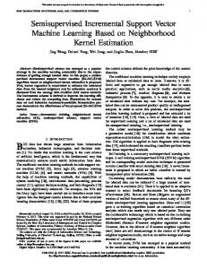
Fig. 2. Sharpe Ratio obtained by the WMV algorithm as a function of β for the two data sets, DJ EuroStoxx 50 (left) and iShare S&P 500 (right), using all the historical data.
respectively. We collected daily historical prices until 13/09/2007, which resulted in data sets with sample sizes of 1856 and 1279 observations. The first 250 data points were used for learning purposes only. A trade is made on each day. The quality of an expert was evaluated by computing the Sharpe Ratio, a measure of risk-adjusted returns. Figure 1 clearly illustrates how the best performing expert changes over time using a sliding window of 22 days (a trading month). Different window sizes produced very similar patterns. The same figure also illustrates the time-varying nature of the ǫ parameter corresponding to the best expert for a randomly chosen sub-period. It clearly emerges that the overall performance may be improved by dynamically selecting or combining experts. In fact, Figure 2 shows that WMV consistently outperforms the average expert for most values of β. More surprisingly, for a wide range of β values, WMV outperforms the best performing expert in the pool by a large margin. Clearly, the meta algorithm is able to strategically combine the expert opinion in a dynamic way. As our ultimate measure of profitability, we compared financial returns generated by WMV with returns generated by a simple Buy-and-Hold (B&H) investment strategy, for both data sets, in Figure 5. Net returns are obtained by taking into account fixed transaction costs and slippage (10 USD and 2 bps, respectively). The figure illustrates the typical market neutral behavior of the trading algorithm. Overall, the correlation coefficient between the returns generated by WMV and the market returns is 0.579 for iShare and 0.521 for EuroStoxx.
5
Conclusions
We have suggested an hybrid algorithm that combines the flexibility of SVR in discovering potential price discrepancies with the robustness of the ensemble learning approach. The final WMV algorithm only depends upon one adjustable
Learning to trade with incremental support vector regression experts 160
7
160 WMV G WMV G
140
140
WMV N
WMV N 120
120 B&H
100 100
Returns %
Returns %
80 80
60
60
40 B&H
40 20 20
0
0
−20
−20
0
200
400
600 Day
800
1000
1200
−40
0
200
400
600
800
1000
1200
1400
1600
1800
Day
Fig. 3. Gross (G) and net (N) returns generated by the WMV algorithm compared to a standard buy-and-hold (B&H) investment strategy for the two data sets, EuroStoxx 50 (left) and iShare S&P 500 (right), using all the available historical data. B&H is a passive, long-only strategy that consists in buying shares of the ETF at the beginning of the investment period and holding them till the end of the period.
parameter, β, for which a default value of 0.7 has proved to work well with very different data sets. Further improvements may be obtained by explicitly forecasting the mispricing series (4), as in [17], and by adopting alternative online learning schemes (e.g. [29]). Preliminary analyzes seems to indicate that the algorithm’s performance degrades only marginally when measurable transaction costs, such as bid-ask spreads and commission fees, are taken into account.
References 1. Y. Bao, Z. Liu, and W. Wang. Forecasting stock composite index by fuzzy support vector machine regression. In Proceedings of the Fourth International Conference on Machine Learning and Cybernetics, 2005. 2. A. N. Burgess. Applied quantitative methods for trading and investment, chapter Using Cointegration to Hedge and Trade International Equities, pages 41–69. Wiley Finance, 2003. 3. D. Cao, S. Pang, and Y. Bai. Forecasting exchange rate using support vector machines. In Fourth International Conference on Machine Learning and Cybernetics, 2005. 4. G. Cauwenberghs and T. Poggio. Incremental and decremental support vector machine learning. volume 13, pages 409–123. Cambridge, 2001. 5. N. Cesa-Bianchi and G. Lugosi. Prediction, learning, and games. Cambridge University Press, 2006. 6. B. R. Chang and H. F. Tsai. Forecast approach using neural network adaptation to support vector regression grey model and generalized auto-regressive conditional heteroscedasticity. Expert Systems with Applications: An International Journal, 34:925–934, 2008. 7. N. Cristianini and J. Shawe-Taylor. An Introduction to Support Vector Machines. Cambridge University Press, 2000.
8
Giovanni Montana and Francesco Parrella
8. R.J. Elliott, J. van der Hoek, and W.P. Malcolm. Pairs trading. Quantitative Finance, pages 271–276, 2005. 9. V. V. Gavrishchaka and S. Banerjee. Support vector machine as an efficient framework for stock market volatility forecasting. Computational Management Science, 3(2):147–160, 2006. 10. Y. He, Y. Zhu, and D. Duan. Research on hybrid arima and support vector machine model in short term load forecasting. In Proceedings of the Sixth International Conference on Intelligent Systems Design and Applications, 2006. 11. W. Huang, Y. Nakamori, and S. Wang. Forecasting stock market movement direction with support vector machine. Computers & Operations Research, 2004. 12. H. Ince and T. B. Trafalis. A hybrid model for exchange rate prediction. Decision Support Systems, 42:1054–1062, 2006. 13. P. Laskov, C. Gehl, and S. Kruger. Incremental support vector learning: analysis, implementation and applications. Journal of machine learning research, 7:1909– 1936, 2006. 14. N. Littlestone and M.K. Warmuth. The weighted majority algorithm. Information and Computation, 108:212–226, 1994. 15. J. Ma, J. Theiler, and S. Perkins. Accurate on-line support vector regression. Neural Computation, 15:2003, 2003. 16. M. Martin. On-line support vector machine regression. In 13th European Conference on Machine Learning, 2002. 17. G. Montana, K. Triantafyllopoulos, and T. Tsagaris. Data stream mining for market-neutral algorithmic trading. In Proceedings of the ACM Symposium on Applied Computing, pages 966–970, 2008. 18. G. Montana, K. Triantafyllopoulos, and T. Tsagaris. Flexible least squares for temporal data mining and statistical arbitrage. Expert Systems with Applications, doi:10.1016/j.eswa.2008.01.062, 2008. 19. G. Nalbantov, R. Bauer, and I. Sprinkhuizen-Kuyper. Equity style timing using support vector regressions. Applied Financial Economics, 16:1095–1111, 2006. 20. J. G. Nicholas. Market-Neutral Investing: Long/Short Hedge Fund Strategies. Bloomberg Professional Library, 2000. 21. F. Parrella and G. Montana. A note on incremental support vector regression. Technical report, Imperial College London, 2008. 22. J. Shawe-Taylor and N. Cristianini. Kernel Methods for Pattern Analysis. Cambridge University Press, 2004. 23. F. Tay and L. Cao. ǫ-descending support vector machines for financial time series forecasting. Neural Processing Letters, 15:179–195, 2002. 24. V. Vapnik. The Nature of Statistical Learning Theory. Springer, 1995. 25. G. Wabha. Spline models for observational data, volume 59 of CBMS-NSF Regional Conference Series in Applied Mathematics. SIAM, 1990. 26. W. Wang. An incremental learning strategy for support vector regression. Neural Processing Letters, 21:175–188, 2005. 27. Y. Wen and Lu B. Advances in Knowledge Discovery and Data Mining, chapter Incremental Learning of Support Vector Machines by Classifier Combining, pages 904–911. Springer Berlin / Heidelberg, 2007. 28. J. Weng, Y. Zhang, and W. S. Hwang. Candid covariance-free incremental principal component analysis. IEEE Transactions on Pattern Analysis and Machine Intelligence, 25(8):1034–1040, 2003. 29. R. Yaroshinsky, R. El-Yaniv, and S. Seiden. How to better use expert advice. Machine Learning, 55(3):271–309, 2004.