ent approaches have been provided, that is a numeric and a binary implementation ... As an example, if the binary option has been selected then three tables.
An OpenGIS®-Based Approach to Define Continuous Field Data Within a Visual Environment Luca Paolino, Monica Sebillo, Genoveffa Tortora, and Giuliana Vitiello Dip. di Matematica e Informatica, Univ. di Salerno, Italy {lpaolino, msebillo, tortora, gvitiello}@unisa.it
Abstract. Many continuous phenomena affect everyday human life. In this paper, the issue of continuous field management has been faced under several points of views, from the design to the implementation stage. The resulting environment provides domain experts with a formal visual approach to conceptually depict mini-worlds of interest embedding spatial data. It is based on an extended version of the OpenGIS standard architecture, thus guaranteeing a natural integration with solutions derived by previous conventional approaches.
1 Introduction One of most fervent research areas in the field of information system is certainly the management of spatial data, that is all aspects dealing with description, definition, design, implementation and querying of data whose main feature is the spatial positioning. In fact, in the last decade, authors, standardization agencies, companies, public administrations have produced a huge quantity of work about this topic embracing every single aspect. As an example, Spatial ER [3] is a data model able to design spatial schemas at a conceptual level, the OpenGIS SQL [10] and SQL3 [7] cover several geographic aspects related to query languages, architectures and implementation details. ArcGIS, MAPGUIDE and Grass are tools able to implement spatial databases and perform spatial analysis. However, they basically centred their attention on data representing “things”. In other words, they deal with discrete objects (e.g., buildings, bridges, etc.) disregarding continuous fields which are often subjects of geographic studies. The concept of field originates from physics and describes an entity distributed over a space A, whose properties are functions of space coordinates. Formally, a function f f : D ⊆A →V, which assigns every location sbelonging toDa unique value f(s) ∈ V, is called a continuous field on D. D ⊆ A represents the domain of f and V corresponds to its range of values (or value domain). Generally, continuous fields are useful to represent phenomena or status which change over time and space regarding the Earth’s surface, such as temperature, pressure, wind, etc. As for continuous fields, some work has been presented in the recent past. [5] and [6] describe an architecture to manipulate fields based on design patterns, [8] and [1] describe a SQL language which allow users to query continuous data as well as spaS. Bres and R. Laurini (Eds.): VISUAL 2005, LNCS 3736, pp. 83 – 93, 2005. © Springer-Verlag Berlin Heidelberg 2005
84
L. Paolino et al.
tial one, and finally, [9] is a visual query language providing means to help nonexpert users to manipulate continuous data. In this paper, the issue of continuous field management has been faced under several points of views, starting from the design stage to the implementation, passing through the description of a Rapid Application Development (RAD) tool able to support users in the task of schema construction. The design stage is based on the previous Calkins’s experience [3], who adapted the ER model in order to manage discrete spatial data using three new entities and two relationships. In particular, he proposed a regular entity able to represent simple spatial information, a multipurpose entity which allows for multiple geometric representations and a temporal entity which can be used to represent data that change over time. As for the relationships, they are based on topological properties such as connectivity and on the geometric coordinates such as inclusion, containing, etc. In our work, this model has been further extended in order to involve two new entities, named continuous and temporal continuous entity able to describe continuous field at a conceptual description level. In order to help the construction of schemas following such a model, a RAD application tool is provided. It gives users the ability to describe schemas through simple interactions and, successively, to export them into both popular interchange file formats, such as SQL scripts and XML schema, and raster formats, such as JPG to support documentation tasks. The generation of SQL scripts relies on the definition of a novel architecture which is based on the OpenGIS standard. It is able to store continuous data as well as discrete data. Such a choice has been done because the OpenGIS standard is already used in many geographic database management systems such as ARCGIS, MySQL and ORACLE. This should allow GIS designers to become quickly familiar with the novel architecture. The remainder of the paper is organized as follows. Section 2 presents the conceptual model describing continuous and discrete data. The RAD tool is shown in Section 3, and finally, the architecture for spatial data is presented in Section 4. Some final remarks conclude the paper.
2 The Conceptual Model One of the most important aspects of database development is the adoption of an appropriate representation that allows to describe data in a completely rigorous and unambiguous fashion so that users and designers agree on data definitions. Researchers have developed several data models such as ER [4] and UML[2], which allow to visually construct intuitive schemas. However, such models are not able to describe all typologies of data and sometimes their symbology is not sufficient to represent data in an abstract way, so that implementation details are needed, in order to make the representation fully functional. This is particularly true when talking about geographic databases, where the cited data models are not able to provide a high level representation for spatial relationships and entities, hence forcing to enrich the schema with implementation details which should instead be hidden at this stage of data modelling.
An OpenGIS®-Based Approach to Define Continuous Field Data
85
In order to overcome such a limitation, Calking introduced the Spatial ER model, which includes graphical notations for spatial entities and relationships [3]. Moreover, it allows to hide implementation details about topology, such as connectivity and contiguity. In the Spatial ER model, regular entities describe spatial “things” which have attributes and are spatially related to each other. In other words they can be either discrete objects (e.g., a building, a bridge, a household, a business, etc.) or abstract objects defined in terms of the space they occupy (e.g., a land parcel, a timber stand, a wetland, a soil type, a contour, etc.). Since in geographic databases it is often the case that the same spatial object has to be represented using different geometric data types, depending on the specific purposes, a new spatial entity named multipurpose entity has been introduced in the model. An example of multipurpose entity is given by a urban street system. It may require that each street segment (the length of street between two intersecting streets) be held in the GIS both as a single-line street network to support address geocoding., and as a double-line (or polygon) street segment for cartographic display. Another entity has been provided to represent regular entities which may change over time. This may include for example a cadastral parcel whose boundary has changed as an effect of a testamentary succession. So, a temporal entity is used to model the temporal evolution of spatial objects. Consequently, three symbols are defined to represent entities: entity(regular); entity(multipurpose); and entity(temporal), as illustrated in Figure 1. The internal structure of the entity symbol contains the name of the entity and additional information indicating the corresponding geometry (point, line or polygon), a code indicating whether the topology of each instance is included or it must be computed at run-time, and a code indicating that the relationships derived using spatial operations are expressed in terms of geographic coordinates (see Figure 2). We have further extended the Spatial ER model in order to manage continuous field data as well as geometric ones using the ER notation.
Fig. 1. The correspondence between the ER and Spatial ER models
86
L. Paolino et al.
Fig. 2. The entity internal structure
Fig. 3. (a) the continuous entity internal structure, (b) the temporal continuous entity representation
As a matter fact, when we deal with continuous fields we cannot talk about “things” because in most cases we describe the perception of a status, such as temperature, pressure, wind and so on, which can change over time and space. Consequently, the spatial management of geographic data through Spatial ER is no longer sufficient. In order to complete the data model with continuous fields, the entity shown in Figure 3(a) has been added. The graphical representation of a continuous entity differs from the regular entity for the cloud drawn around the entity which recalls the concept of continuous data and the additional box, named N, which indicates the continuous field dimensions, namely 1 for a scalar field (e.g., temperature) and n for an n-dimensional vector (e.g., wind). Similarly to regular entities, continuous entities need also a representation able to model changes over time. For example, we need to use a temporal continuous entity to store data received from detection stations at different times. In order to be consistent with respect to the representation of discrete temporal entities, we have chosen to represent a continuous temporal entity drawing three clouds around the entity, as shown in Figure 3(b). In the following, we describe the visual environment for schema editing, which embeds the described extension of the Spatial ER model.
3 The RAD Schema Environment The environment described in the present section allows users to build schemas according to the spatial model we have illustrated so far. It has been implemented using
An OpenGIS®-Based Approach to Define Continuous Field Data
87
the Java programming language which allows us to easily distribute the software over multiple platforms with no need to implement different versions. The interface (see Fig.4) is divided into three parts, a menubar, a toolbar, and a working area. By means of the menubar the user can either perform simple file operations such as open, close, save, save as, etc, and simple editing operations on components contained into the working area such as cut, copy, paste, or select the architecture according to which the spatial database should be implemented. As for the latter, two different approaches have been provided, that is a numeric and a binary implementation which will be exhaustively described in the following. The toolbar allows users to select the items which are involved in the schema construction and to translate them into an intermediate data definition language. It is divided into four groups of buttons. The first set can be used to quickly recall the file operations. The second and the third sets represent entities and relationships, respectively, and will be used to compose the schema according to the requirements. In particular, the first group contains buttons indicating simple alphanumeric entities, discrete spatial entities and continuous spatial entities. In order to relate them, it is possible to use the relationships depicted in the second group, which include conventional relationships, relationships derived using spatial operations, relationships represented by topology and generalization. Similarly to common RAD tools, such buttons can be selected and visually located inside the working area, by simple drag-and-drop operations. The last group represents a set of buttons which provides users with the ability to export the schema into several interchange formats, such as SQL and XML. Also a raster format can be generated for documentation purposes as a JPG image. The final part composing the environment is the working area where the user is enabled to build the spatial schema.
Buttons to select entities for continuous and discrete data
Buttons to export schema in XML, JPG, SQL representations Buttons to select spatial and generalization relationships
Fig. 4. A screenshot showing the environment embedding the extended spatial ER
88
L. Paolino et al.
Once the elements are dropped into the working area, their properties are specified adding the corresponding attributes while graphical features such as colours, width, height and line size can be modified by simple interactions. Figure 4 illustrates a simple schema using continuous entities. It refers to a set of parcels, containing both some buildings and some detection stations which acquire the temperature at terrain level. In particular, it is required that temperature samplings are collected at regular time periods, usually, every 8 hours. The resulting diagram contains five elements, two discrete entities (Parcel, Building) and one temporal continuous entity (Temperature), which are connected by two Contains relationships implemented using spatial operations. The environment performs automatic controls on the diagram detecting possible incompleteness (due, e.g., to missing attributes or pending relationships). The user can then export the described schema into a format manageable by a DBMS, translating it into a SQL script by the SQL button. In particular, the environment allows to transform the visual schema into a set of CREATE statements following an extension of the OpenGIS standard to continuous field data, which we propose in [8]. The resulting SQL script depends also on the architecture previously selected in the File>Option item. As an example, if the binary option has been selected then three tables will be created apart from the catalogue and spatial reference system tables. Figure 5 shows the script fragment representing the creation of the Temperature temporal continuous field table, which is based on the following structure: CREATE TABLE ( GID NUMBER NOT NULL PRIMARY KEY, XMIN , YMIN , XMAX , YMAX , WKB_CONTINUOUS_FIELD VARBINARY, )
where − GID is an integer representing a primary key. − XMIN, …, YMAX is the minimum bounding box containing the domain, − WKB_CONTINUOUS_FIELD represents a binary attribute which will contain the continuous field information according to the Well Known Binary representation defined in [10], − represents possible alphanumeric attributes and
Fig. 5. The SQL script defining the temperature continuous field
An OpenGIS®-Based Approach to Define Continuous Field Data
89
4 The Architecture for Spatial Data Following the approach discussed in Section 2, a novel architecture, shown in Figure 6, has been developed in order to contain feature tables including both geometric and continuous data. It is based on the OpenGIS standard architectures depicted in [10] and allows users to store information according to two different methodologies, that is using either numeric or binary attributes. In order to model also continuous data, the basic architecture has been extended with tables 3 and 4 for storing numeric or binary sampling values, respectively.
Fig. 6. The architecture to store geometric and continuous field data
In the following a description of the tables shown in Figure 6 is given. FEATURE_TABLEs (Table 5). Like the OpenGIS, they contain information about objects containing both spatial and non-spatial attributes. The correspondence between the feature instances and either the geometries or the continuous field instances is accomplished through a foreign key which is stored in the ID attribute of the feature table. With respect to the OpenGIS, this foreign key not only refers to the ID primary keys of Tables 1 and 2 (already existing in the basic architecture), but also to the ID attributes of Tables 3 and 4, which we introduce to extend the architecture. Information about continuous fields is stored either combining GEOMETRY_ COLUMNS (Table 1) and SURFACE_COLUMNS (Table 3) or using the CONTINUOS_ FIELD_COLUMNS (Table 4). In particular, according to the numeric specification, Table 1 stores the geometry corresponding to the continuous field domain, while Table 3 the field surface. As for the binary representation, Table 4 contains information about the whole field.
90
L. Paolino et al.
From an implementative point of view, each primitive element in the geometry of Table 1 is distributed over some adjacent rows in the table ordered by a sequence number (SEQ), and identified by a primitive type (ETYPE). Each geometry identified by a key (ID), consists of a collection of primitive elements numbered by an element sequence (ESEQ). Finally, the Xi, Yi attributes indicate the geometry vertices. In Table 3, for each primitive element identified by the (ID, ESEQ) pair, a set of sampled points (Xi, Yi, Zi) is given. Similarly to the geometries in Table 1, sampled points may be distributed over multiple rows which will be ordered by the CSEQ attribute. The evaluation method and the time evaluation period are stored in the EVALMETH and TIMEEVAL attributes, respectively. As for the binary, the basic OpenGIS architecture has been enriched with a new table (Table 4) able to entirely store continuous fields using a Well-Known Binary (WKB) representation. The WKB Representation for Geometry and Continuous field is obtained by serializing an instance as a sequence of numeric types drawn from the set {Unsigned Integer, Double} and then serializing each numeric type as a sequence of bytes using one of two well defined, standard, binary representations for numeric types (NDR, XDR). The specific binary encoding (NDR or XDR) used for an instance representation is described by a one byte tag that precedes the serialized bytes. The only difference between the two encodings of geometry is the byte order, so that the XDR encoding corresponds to the Big Endian order while the NDR encoding corresponds to the Little Endian order. The complete description of the new WKB representation for continuous fields is shown in Figure 7. Each WKB format of a continuous field is composed by: • a byte indicating the order ( 0 for XDR, 1 for NDR), • a wkbtype always set to 8 in order to indicate a continuous field (such a value has been added to standard OpenGIS values in order to integrate the new data types), • two arrays named points and values containing numSamples sampled values, • two values indicating the interpolation method and the evaluation time, respectively. • a domain chosen from the set {WKBPoint, WKBLineString, WKBPolygon, WKBMultipoint, WKBMultiLineString }, which are the domains already described in the OpenGIS standard [10]. In case of a continuous field composed by multiple instances the WKBContinuosField representation is slightly modified. In fact, the wkbtype is set to 9, a num_wkbcontinuosfield value is used to store the instances number of continuous fields composing the collection, and then, an array of num_wkbcontinuous fields contains the continuous fields stored in the simple WKB format. The last two tables are the GEOMETRY_COLUMNS and the SPATIAL_REFERENCE_SYSTEMS. Both already exist in the standard OpenGis, but the GEOMETRY_COLUMNS has been suitably modified to fit the continuous data extension, as described in the following. GEOMETRY_COLUMNS (Table 6) represents a relationship among the table containing the features (Table 5) , the tables containing spatial data (Tables 1, 2, 3, 4) and
An OpenGIS®-Based Approach to Define Continuous Field Data WKBContinuousField { union { byte _order; uint32 wkbtype; //8 uint32 numSamples; Point points[numSamples]; double values[numSamples]; uint32 evaluationmethod; uint32 evaluationtime; union { WKBPoint Point; WKBLineString linestring; WKBPolygon polygon; WKBMultipoint mpoint; WKBMultiLineString mlinestring; } } WKBContinuousFieldCollection collection; }
91
WKBContinuousFieldCollection { ….byte byte_order; ….uint32 wkbtype ………….//9 ….uint32 num_wkbcontinuousfield; ….WKBContinuousField wkbcontinuousfield[num_wkbcontinuousfield]; }
Fig. 7. The WKB representation for Continuous fields and Continuous Field Collection
the reference system (Table 7). As for the FEATURE_TABLE, it is identified by the triplet (F_TABLE_CATALOG, F_TABLE_SCHEMA, F_TABLE_NAME) which uniquely specifies the table following the SQL92 Information schema. The SRID is a foreign key referring to the SPATIAL_REFERENCE_SYSTEMS table. Finally, the STORAGE_TYPE attribute specifies which tables are used to store the geometry or the continuous field. So, • • •
•
if the attribute assumes value 0 then a geometry is stored in Table 1 according to the numeric approach and the triplet of Table 6 (G_TABLE_CATALOG, G_TABLE_SCHEMA, G_TABLE_NAME) is instantiated. if it assumes value 1 then a geometry is stored in Table 2 according to the binary approach and the triplet of Table 6 (G_TABLE_CATALOG, G_TABLE_SCHEMA, G_TABLE_NAME) is instantiated, if it assumes value 2 then a continuous field is stored in both Table 1 and Table 3 according to the numeric approach. In this case, the triplets (G_TABLE_CATALOG, G_TABLE_SCHEMA, G_TABLE_NAME) and (S_TABLE_CATALOG, S_TABLE_SCHEMA, S_TABLE_NAME are instantiated in order to contain references to the tables. if it assumes value 3 then a continuous field is stored in Table 4 according to the binary approach and the triplet of Table 6 (S_TABLE_CATALOG, S_TABLE_SCHEMA, S_TABLE_NAME) is instantiated.
Finally, the attributes MAX_PPR, COORD_DIMENSION and TYPE are described. The first one indicates the MAXimum Point Per Row, that is the number of geometry points stored in a row of Tables 1 and 3. The COORD_DIMENSION indicates the number of dimensions used, which usually corresponds to the number of dimensions in the spatial reference system. Finally, according to [10], the TYPE attribute indicates the type of geometry as follows:
92
L. Paolino et al.
0 = GEOMETRY 1 = POINT 2 = CURVE 3 = LINESTRING 4 = SURFACE 5 = POLYGON
6 = COLLECTION 7 = MULTIPOINT 8 = MULTICURVE 9 = MULTILINESTRING 10 = MULTISURFACE 11 = MULTIPOLYGON
In order to extend it, we add two new items, which represent the CONTINUOUS_FIELD (12) and the CF_COLLECTION (13), respectively.
5 Final Remarks The description of a mini-world which embeds spatial data may be easily accomplished by a domain expert user through the visual environment we propose. Both discrete and continuous spatial data can be modeled by characterizing their properties in terms of attributes and relationships. The resulting schema can then be checked in terms of completeness and translated into commonly used data definition languages. The visual environment is currently being tested on a real environmental application, which will be illustrated during conference presentation. Further properties can be taken into account in future developments, in order to enable users both to describe functional and transactional aspects, and to compose parametric visual queries, thus supporting them along the whole software development.
References 1. Bajerski P., Fraczek J., Mrozek D.: Spatial Distribution Query Language, Procs. of GISIDEA 2004, September 16-18, 2004. Hanoi, Vietnam. 2. Booch G., Rumbaugh J., Jacobson I.: The Unified Modeling Language User Guide, Addison-Wesley. 3. Calkins Hugh W.: Entity Relationship Modeling of Spatial Data for Geographic Information Systems, www.geo.unizh.ch/oai/spatialdb/ergis.pdf 4. Chen P.P.: The entity-relationship model - toward a unified view of data, ACM Transactions on Database Systems, vol. 1(1), March 1976, pp. 9-36. 5. Gordillo S., Balaguer F.: Refining an object-oriented GIS design model: Topologies and th Field data. ACM-GIS '98, Procs of The 6 Int.l Symposium on Advances in Geographic Information Systems. Washington DC, USA, November 6-7, 1998. 6. Gordillo S., Balaguer F. and Das Neves F.: Generating the architecture of GIS applications with design patterns. Procs of the ACM-GIS’97: Advances in Geographic Information Systems. Las Vegas, USA, November 13-14, 1997. 7. ISO/IEC 13249-3:1999, Information technology – Database languages -- SQL Multimedia and Application Packages --Part 3: Spatial, Int. Org. for Std. 8. Laurini R., Paolino L., Sebillo M., Tortora G., Vitello G.: A Spatial SQL Extension for th Continuous Field Querying. Procs of The 28 Annual Int.l Computer Software and Applications Conference - Workshops and Fast Abstracts - (COMPSAC'04), Hong Kong, September 28 - 30, 2004.
An OpenGIS®-Based Approach to Define Continuous Field Data
93
9. Laurini R., Paolino L., Sebillo M., Tortora G., Vitiello G.: Phenomena - A Visual Query Language for Continuous Fields. Procs of ACMGIS 2003 Advances in Geographic Information Systems. New Orleans, Louisiana, USA, 2003. 10. OpenGIS Simple Feature Specification for SQL, http://www.opengeospatial.org/docs/99049.pdf