motion of HRP-2FX to minimize a performance index, and the optimality has been verified ..... a high-jump mattress made of polyurethane foam. Figure 11 shows ...
Proceedings of the 2007 IEEE/RSJ International Conference on Intelligent Robots and Systems San Diego, CA, USA, Oct 29 - Nov 2, 2007
TuB5.3
An Optimal Planning of Falling Motions of a Humanoid Robot Kiyoshi FUJIWARA, Shuuji KAJITA, Kensuke HARADA, Kenji KANEKO, Mitsuharu MORISAWA, Fumio KANEHIRO, Shinichiro NAKAOKA, and Hirohisa HIRUKAWA
Abstract— This paper studies an optimal planning of falling motions of a human-sized humanoid robot to reduce the damage of the robot. We developed a human-sized robot HRP-2FX which has a simplified humanoid robot shape with seven d.o.f. and can emulate motions in the sagittal plane of a humanoid robot. An optimal control is applied to generate the falling motion of HRP-2FX to minimize a performance index, and the optimality has been verified by the experiments on HRP-2FX.
I. INTRODUCTION Biped humanoid robots have several advantages over wheeled mobile robots. They can step over obstacles and go up and down stairs. On the other hand, the robots have a major disadvantage. They may fall over and then damage severely. This is one of the crucial barriers for practical application of humanoid robots. Humanoid robots cannot be accepted for use in society unless this problem is overcome. Compared with quadruped walking robots or wheeled ones, the center of gravity of a biped-walking robot is located at a relatively high position and the size of the convex hull of the feet is smaller. A biped humanoid robot is essentially an unstable structure, and so little can be done to prevent the robot from falling over[1]. In addition, the robot may be damaged seriously enough to prevent it from walking thereafter, since the impact between the robot and the ground can be large. The bigger the humanoid robot, the more serious the damage can be. It is therefore important to address this problem. The goal of our research is to prevent physical damage that would disable the locomotive ability of the robot, thus giving it a chance to stand up again. For this purpose, we proposed a safe falling motion control strategy to minimize damage to humanoid robots, in which we have shown how to control falling[2], [3]. In order to decrease damages, we have to consider a tradeoff between the landing impact and the position as well as the stability after the landing and the position. In this paper we investigate this problem. An optimal planning method is applied to design safe falling motions. The effectiveness of the proposed method was verified by the experiments using a human-sized humanoid robot which has a simpler shape and less degrees of the freedom specially designed for falling motion experiments. The authors are with Intelligent Systems Research Institute, National Institute of Advanced Industrial Science and Technology (AIST), Tsukuba Central 2, 1-1-1 Umezono, Tsukuba, Ibaraki, Japan. e-mail: { k-fujiwara, s.kajita, kensuke.harada, k.kaneko, m.morisawa, f-kanehiro, s.nakaoka, hiro.hirukawa }@aist.go.jp
1-4244-0912-8/07/$25.00 ©2007 IEEE.
Fig. 1.
HRP-2FX
This paper is organized as follows. Section II overviews humanoid robot HRP-2FX and dynamics model of forward falling, Section III presents a modeling of a foward falling motion. Section IV presents an an optimization technique. Section V is about results of optimization. Section VI shows results of experiments. And section VII concludes the paper. II. HRP-2FX We have tried many experiments of falling over motion control using human-sized humanoid robot HRP-2P[4]. But it is not reasonable to use such a human-sized humanoid robot with full specifications for preliminary falling experiments, since it includes mechanisms more than necessary to the experiments. It is easy to damage the robot by the experiments in which a large impact should be applied at a landing, and it is difficult and expensive to maintain it. Therefore, we have developed a simplified humanoid robot HRP-2FX with a minimum mechanism which is essential for the falling experiments (See Fig. 1)[5]. HRP-2FX is designed to emulate the motions in the sagittal plane of HRP-2P/HRP-2, and therefore it can be used for the experiments of forward and backward falling motions. The remained configuration of HRP-2FX follows that of HRP-2P/HRP-2 including the length of the links, the movable ranges of the joints, actuators, sensors and electronics. Each joint are corresponding to the pitch joints of HRP-2P, except for the head and wrists joints(Table I). These joints are located at the ankle, knee, hip, chest, shoulder and both elbows. These configurations make the control software OpenHRP[6] to be applicable with small modifications. The
456
TABLE I
falling robot by the single inverted pendulum model[3] since the landing position and the COG are close. When the robot falls forward, however, it lands at the knee which is far from the COG. Therefore, we cannot model a robot falls forward by the single inverted pendulum.
Specifications of HRP-2P & HRP-2FX
Legs
Waist Arms Hands Neck Height (standing straight) Weight
HRP-2P 6 D.O.F./Leg (Hip:3 Knee: 1 Ankle: 2) Upper leg length: 0.3[m] Lower leg length: 0.3[m] Ankle height: 0.1 [m] 2 D.O.F (Yaw:1 Pitch:1) 6 D.O.F./Arm (Shoulder:3 Elbow:1 Wrist:2) 1 D.O.F./Hand 2 D.O.F. (Yaw:1 Pitch:1) 1.58 [m] (floor–top) 0.81 [m] (floor–center of mass) Total 58 [kg]
HRP-2FX 3 D.O.F./Leg (Hip:1 Knee: 1 Ankle: 1) Upper leg length: 0.3[m] Lower leg length: 0.3[m] Ankle height: 0.09 [m] 1 D.O.F (Pitch:1) 3 D.O.F./Both (Shoulder:1 Elbow:2)
A. Modeling of the dynamics Let us use a quadruple inverted pendulum model as shown in Fig. 3. The links are numbered from 0 to 3 from the lowest
1.49 [m] (floor–top) 0.835 [m] (floor–center of mass) Total 28 [kg]
power supplier and computers are placed outside, since it does not need to be self consistent. In this case, there is no requirement to consider any actions in a lateral direction. So, this robot has only one wide leg and the right and the left upper arms are driven by one servomotor as one link. The angular rate sensors of yaw and roll axis have also been omitted. The forearms are driven by independent servomotors, which are synchronized by position control. To obtain the similar dynamic falling motion, we designed HRP-2FX to be approximately one half of HRP-2P (Fig.2). Then the mass distribution of the leg of HRP-2FX is comparable to that of a leg of HRP-2P, and that of the body is about a half of HRP-2P.
Fig. 3.
Dynamics model of a forward falling motion
one, and link 0 corresponds to the links between the toe and the knee in the original robot, link 1 to the upper leg, link 2 to the torso and link 3 to the arms respectively. We separate the falling motion into two stages. Stage 0: This is the motion from the standing state to the landing of the knee. The position of the tiptoe is fixed on the ground. We define joint 0 be the rotational axis at the tiptoe. Stage 1: This is the motion after the landing of the knee until the landing of the arm. The position of the knee is fixed on the ground. We define joint 1 be the rotational axis at the knee. The equations of motion can be written as
Fig. 2. In the sagittal plane, HRP-2FX is nearly equal to a half of HRP-2P
There are soft cushions at each joint to absorb landing impacts, and all weak elements such as the motors are protected by the frame. The design can make HRP-2FX emulate the falling motion of HRP-2P/HRP-2 in the sagittal plane safety at a low cost. III. M ODELING OF A FORWARD FALLING MOTION Now, let us discuss a forward falling motion of HRP-2FX. In the case of backward falling motion, we could model the
457
2 Aθ¨ + B θ˙ + C sin θ = Du,
(1)
A
=
{Lij cos (θi − θj )} ,
(2)
B C
= =
{Lij sin (θi − θj )} , −diag(gG),
(3) (4)
D
=
KT K , � �2 m M α α �2n=0 n 2ni nj n=0 Mn αni + Ii
Lij
=
(5) (i �= j) , (i = j)
(6)
α0
α1
0 0 r0 0 R0 r1 R0 R1 r2 R0 R1 R2 r0 − R0 0 0 r1 0 R1 0 R1 � α0 (Stage0) α1 (Stage1) 1 0 0 0 −1 1 0 −1 1 0 0 −1 0 0 0 1 0 0 , 0 1 0 0 0 1 Kθ,
=
=
α =
K
=
Km
=
q
=
, 0 0 , 0 1
βs βc
(12)
T
(14)
T
(15)
T
(16)
T
(17)
=
[θ0 θ1 θ2 θ3 ] ,
q
=
[q0 q1 q2 q3 ] ,
I
=
[I0 I1 I2 I3 ] ,
u
=
[u1 u2 u3 ] ,
T
(18)
where θn is the angle of the link n from the vertical line and qn is the relative angle between the consecutive links at joint n, In is the moment of inertia of link n, and un is the torque input to the n th joint. Note that joint 0 is a free joint and no input can be specified. The same equation can be used for both of the stages by switching the matrix α, which is α0 for stage 0, and is α1 for tage 1. Table II shows the parameters of this model and initial stats based on HRP-2FX.
∂T − ∂T + = + − + P, ∂ ξ˙ ∂ ξ˙
r[m] 0.20 0.15 0.31 0.23
joint0 joint1 joint2 joint3
q(0)[deg] 4.8 −15.8 4.4 4.4
M [kg] 4.166 2.076 15.96 5.57
q(0)[deg] ˙ q˙0 (0) 0 0 0
(21)
where x˙j ,z˙j are the horizontal and the vertical components of the landing point velocity. In stage 0, the landing point is the knee; when it is necessary to distinguish it, we transcribe ˙ . In stage 1, the landing point is the tip of them into x˙j1 ,zj1 the arm; we transcribe them into x˙j4 ,zj4 ˙ . Since we assume the landing to be perfectly inelastic, the velocity after the impact becomes �T
+ + (23) ξ˙ := θ˙ 0 0 . The kinetic energy T is given by
Q 1 ˙T A ˙ M 0 ξ, T = ξ QT 2 0 M
(24)
where the matrix Q is G0 cos θ0 G1 cos θ1 Q= G2 cos θ2 G3 cos θ3
−G0 sin θ0 −G1 sin θ1 . −G2 sin θ2 −G3 sin θ3
(25)
By substituting Eq.(22),(23),(24) and (25) into Eq.(21), we obtain the equation for the velocity change at the impact.
−
� � A Q 0 θ˙ − + A x˙j M 0 θ˙ = + Px , (26) QT QT Pz z˙j − 0 M
I[kgm2 ] 0.321 0.239 0.724 0.301 qmin [deg] −4.2 −150.8 0 0
(20)
where T is the kinetic energy and P is the applied impact. In the case of landing on the knee, we use P1 and in the case of landing on the arm, we use P4 as P . We put − to the states immediately before the impact and put + to the states immediately after the impact. ξ˙ is the generalized velocity. Let us define the velocity before the impact as �T
− − − , (22) ξ˙ := θ˙ x˙ − j z˙ j
Parameters of the model R[m] 0.37 0.30 0.53 0.54
= M (α diag(sin θ)) = M T (α diag(cos θ)).
When the knee or the arm of the robot hits the ground, the speed of all joints changes immediately by the landing impact. Generally, impact dynamics can be represented by the following equation.
TABLE II
link0 link1 link2 link3
(19)
T
B. Impact dynamics at landing
(11)
[M0 M1 M2 M3 ] ,
2
¨ − βc θ˙ + gM, = −βs θ
(8)
(13)
θ
fz
(10)
α M,
=
floor reaction force fz during the falling motion given as (7)
(9)
T
G =
M
0 0 , 0 r3 0 0 0 0 , r2 0 R2 r3
qmax [deg] 90.0 24.2 125.0 200.0
In addition, we can calculate the vertical component of the
where Px and Pz are the horizontal and the vertical components of the impulse P at the landing point, respectively (Fig. 4, left). We can calculate the change of the joint velocities from the first row of Eq.(26) as � − �� � ˙θ + = A−1 Aθ˙ − + Q x˙j − . (27) z˙j
458
The rest part of Eq.(26) gives the impulse at an impact moment. � �� � � � + − M 0 x˙j1 − Px = QT θ˙ − QT θ˙ − . 0 M Pz zj1 ˙ − (28)
with the terminal condition p[T ]
=
−
�
∂JT ∂x
�
.
(36)
We can easily find p by integrating Eq.(35) in the reversing time from t = T to 0. Based on the dynamics, gradient function Ju can be obtained by �T � � � ∂f ∂Jt . (37) p+ Ju = − ∂u ∂u The optimal input u can be found by the iterations using Ju as the gradient function. We applied the steepest descent method to find the optimal input u. A. The Performance Indexes We set the performance index at final time T as
Fig. 4.
Landing model of a forward falling motion
JT The angular momentum immediately after the landing Lj1 + is given by � � �T � + x˙c + xc − xj + (29) Lj = M + I θ˙ . zc − zj −z˙c +
where xc ,zc are the COG position of the whole robot body. Lj can be written as Lj1 in the case of landing on the knee and be written as Lj4 in the case of arm. Let us call them an excessive angular momentum. To get a stable and safe landing, it is desirable to have the excessive angular momentum after the impact as small as possible.
x f (x, u)
= := :=
f (x, u), � � θ , θ˙ A
−1
2 (Du − B θ˙ − C sin θ)
Let J be the total performance index defined by � T Jt dt, J = JT +
KL (JL )2 + KM (JM )2 ,
JL
(33)
KF (JF )2 + KL (JL )2 + KM (JM )2 .
(40) (41) (42) (43)
= lower(q1 , qmin1 ) + upper(q1 , qmax1 ) + lower(q2 , qmin2 ) + upper(q2 , qmax2 )
(45)
JM1
+ lower(zj3 , 0) + lower(zj4 , 0), = lower(zj0 , 0) + lower(zj2 , 0) + lower(zj3 , 0) + lower(zj4 , 0), � JM0 (Stage0) = , JM1 (Stage1)
(46)
JM
(34)
(39)
JM0
0
where p is the co-state that has the same dimension as x. The dynamics of p can be given by � � ∂H p˙ = − ∂x � � �T � ∂f ∂Jt = − p+ , (35) ∂x ∂x
=
+ lower(q3 , qmin3 ) + upper(q3 , qmax3 ), (44) = lower(zj1 , 0) + lower(zj2 , 0)
. (32)
where Jt is the state at time instance t (0 ≤ t ≤ T ) and JT that at the final time T . To minimize J, we define a Hamiltonian by H = pT f − Jt ,
(38)
The evaluating parameters are given as � P1 (Stage0) JA = , P4 (Stage1) � Lj1 + (Stage0) JB = , Lj4 + (Stage1) � zj1 (Stage0) , JP = zj4 (Stage1) JF = lower(fz , 0),
(31) θ˙
+
Jt
(30)
KA (JA )2 + KB (JB )2 + KP (JP )2 + KF (JF )2
where K∗ (∗ = A, B, P, F, L, M ) are the weights for tuning motion. For example, the weight KP works in order to restrict the landing may occur at time T . Also, we set the performance index along the falling trajectory as
IV. O PTIMIZATION We apply an optimization method[7][8] which is based on the Pontryagin’s minimum principle. It is followed, Equation (1) can be rewritten as x˙
=
lower(X, Xmin ) :=
upper(X, Xmax ) :=
(47)
Xmin − X + 1), KS 1+ (48) 1 X − Xmax + 1), ( KS 1 + eKE (Xmax −X) (49) 1
eKE (X−Xmin )
(
where JF is to keep positive floor reaction force and JL is to keep the joint angles within the limitation. JM is used to
459
guarantee the first landing of the desired point. KE and KS are the parameter for the sloped sigmoid function. We independently optimized Stage 0 and Stage 1 of a forward falling motion. Table III shows the weights used for optimizations. TABLE III Weight factors for evaluation weights KP 1000 KF 1 KL 100 KM 200 KE 10 KS 10
limits UP 0.001 UF 50 UL 0.1 UM 0.4
B. A viability check Even if it is a motion provided by optimization, there is the case that an unrealizable result is obtained. For example, there can be the violation of the joint movable range or the large error of the landing timing. They can be controlled by tuning weights, but are not enough. In order to reject inapparopriate results, we introduce a viability check using the same parameters of the performance index, �� � T JF dt ≤ UF V = (JP (T ) ≤ UP ) ∩
Fig. 5.
A result of a simulation (q˙0 (0) = 90[deg/s])
0
∩
��
T
JL dt ≤ UL
0
∩
��
�
T
JM dt ≤ UM
0
�
,
(50)
where UP , UF , UL and UM are threshiold for eagh evaluating parameters. When V =TRUE, the provided motion can be said to be feasible movement. C. Searching the final time T This technique demands terminal times T0 , T1 as given parameter of the optimization. On the other hand, it is obvious that T0 and T1 have strong influence on the generated motion. Therefore we determine the optimal terminal times by the following algorithm. (i) Stage0 optimization for a range of T0 = 0.1 ∼ 0.5[s] every 0.01[s] (ii) Filtering by viability check V (iii) Choose T0 that gives the minimum JA (iv) Stage1 optimization for a range of T1 = 0.1 ∼ 0.4[s] every 0.01[s] using the terminal condition of optimal Stage0 as the initial condition (v) Filtering by V of the result of the (iii) (vi) Choose T1 that gives the minimum JA The falling motion and its timing which result minimum impact can be obtained by the above mentioned procedure.
Fig. 6.
Optimal motion of each joints
V. T HE RESULTS OF OPTIMIZATION Figure 5 shows the stick diagrams of the optimal motion whose initial condition is shown in Table II and q˙0 (0) = 90[deg/s]. In this optimization, we used KA = KB = 0.001 and weights shown in Table III. We can observe a smooth falling motion of the robot. In addition, the COG of whole body is shown by the circle, which bounds at the moment of the knee landing. Figure 6 shows the joint angles of the optimized falling motion. The final time T provided by optimization are T0 = 0.27[s] and T1 = 0.22[s]. A. Initial velocity modifications We calculated the optimal falling motions under different initial speeds. Table IV shows the results of optimization. We can observe a tendency that the robot takes the earlier terminal time T0 , T1 , when q˙0 (0) becomes longer. There is negative correlation between q˙0 (0) and T (Fig. 7). Figure 8, 9 and 10 shows optimized motions when q˙0 (0) =60, 120 and 150.
460
TABLE IV results of optimizations with several q˙0 (0) q˙0 (0) [deg/s] 50 60 70 80 90 100 110 120 130 140 150 160
T0 [s] 0.36 0.34 0.32 0.30 0.27 0.27 0.27 0.27 0.27 0.27 0.27 0.25
T1 [s] 0.37 0.26 0.25 0.23 0.21 0.20 0.19 0.16 0.15 0.14 0.13 0.14
P1 [Ns] 16.1 13.4 12.4 12.6 12.7 14.8 19.0 23.4 27.5 30.7 35.8 34.5
P4 [Ns] 37.7 122.1 118.7 97.0 128.1 81.6 71.1 69.8 58.6 53.0 50.5 54.7
Lj1 [m2 /s] 32.5 37.0 41.7 45.5 45.9 52.7 59.5 64.1 69.3 75.0 82.0 82.2
Lj4 [m2 /s] 16.3 42.6 47.4 38.1 46.7 33.9 41.7 44.5 48.2 52.9 58.7 52.5
Fig. 8.
An optimized motion (q˙0 (0) = 60[deg/s])
Fig. 9.
An optimized motion (q˙0 (0) = 120[deg/s])
Fig. 10.
An optimized motion (q˙0 (0) = 150[deg/s])
�� Fig. 7.
Terminal time T0 , T1 with the change of q˙0 (0)
VI. E XPERIMENTS To evaluate the optimized forward falling motion, we conducted a preliminary experiment using HRP-2FX. Standing HRP-2FX was pushed from the back by hand and started forward falling motions. As soon as the detection the start of the falling motion, the robot started to playback the optimized forward falling motion calculated in advance. To avoid the hardware damage, we tested the falling motion onto a high-jump mattress made of polyurethane foam. Figure 11 shows snapshots of the experiment. We can observe a soft and safe landing motion. Figure 12 shows the link acceleration of the same experiment measured by accelerometers located in right arm and knee of the robot. The robot first landed at 0.51[s] on the knee with peak acceleration of 4.41[G]. It kept rotating around the knee and landed on the hands (tip of the arm) at 0.73[s] with peak acceleration of 5.39[G]. Other peaks of acceleration around at 0.2[s] and 0.4[s] were generated by the servomotors. VII. CONCLUSIONS AND FUTURE WORKS In this paper, we introduced HRP-2FX which was developed to evaluate falling motions of humanoid robots. To minimize the landing impact of a falling motion, we proposed the use of an optimization technique based on variational principle. A quadruple inverted pendulum was used to represent a falling motion with two different stages. We tested the resulted optimal forward falling motion by
HRP-2FX and obtained a smooth and safe landing with moderate impact. Although our current method is based on an off-line optimization, it is indispensable to realize a real-time motion generation for humanoid robots in the real environment. This should be our next target. References are important to the reader; therefore, each citation must be complete and correct. If at all possible, references should be commonly available publications.
461
R EFERENCES [1] Tatsuzo Ishida, Yoshihiro KUROKI, Taro TAKAHASHI, “Analysis of Motions of a Small Biped Entertainment Robot,” Proc. Int. Conf. on Intelligent Robots and Systems(IROS), pp.142-147, 2004. [2] Fujiwara, K., Kanehiro, F., Kajita, S., Kaneko, K., Yokoi, K., Hirukawa,H., “UKEMI: Falling Motion Control to Minimize Damage
Fig. 11.
Fig. 12.
[3]
[4]
[5]
[6] [7] [8]
A falling over motion of HRP-2FX
Landing impact under falling motion control
to Biped Humanoid Robot,” Proc. Int. Conf. on Intelligent Robots and Systems(IROS), pp.2521-2526, 2002. Fujiwara, K., Kanehiro, F., Kajita, S., Yokoi, K., Saito, H., Harada, K., Kaneko, K., Hirukawa,H., “The First Human-size Humanoid that can Fall Over Safely and Stand-up Again,” Proc. Int. Conf. on Intelligent Robotics and Systems(IROS), pp.1920-1926, 2003. Kenji, K., Kanehiro, F., Kajita, S., Yokoyama, K., Akachi, K., Kawasaki, T., Ota, S., Isozumi, T., “Design of Prototype Humanoid Robogics Platform for HRP,” Porc. Int, Conf, on Intelligent Robots and Systems(IROS), pp.2431-2436, 2002. Fujiwara, K., Kajita, S., Harada, K., Kaneko, K., Morisawa, K., Kanehiro, F., Nakaoka, S., Hirukawa, H., “Towards an Optimal Falling Motion for a Humanoid Robot,” Proc. of 2006 IEEE-RAS International Conference on Humanoid Robots, pp.524-529, 2006. Hirukawa, H., Kanehiro, F., Kajita, S., “OpenHRP: Open Architecture Humanoid Robotics Platform,” Intr. Symposium on Robotics Research (ISRR), Melbourne, November 2001. M. J. D. Powerll (Ed.),“Nonlinear Optimization,” 1981, NATO Conference Series, Academic Press(1982) Howie Choset et al. ,“Principles of Robot Motion : theory, algorithms, and implementations,” MIT Press, (2005).
462