An Optimal Probabilistic Forwarding Protocol in Delay Tolerant Networks. Cong
Liu and Jie Wu. Department of Computer Science and Engineering.
An Optimal Probabilistic Forwarding Protocol in Delay Tolerant Networks Cong Liu and Jie Wu
Department of Computer Science and Engineering Florida Atlantic University Boca Raton, FL 33431
{cliu8@, jie@cse}.fau.edu
ABSTRACT Due to uncertainty in nodal mobility, DTN routing usually employs multi-copy forwarding schemes. To avoid the cost associated with flooding, much effort has been focused on probabilistic forwarding, which aims to reduce the cost of forwarding while retaining a high performance rate by forwarding messages only to nodes that have high delivery probabilities. This paper aims to provide an optimal forwarding protocol which maximizes the expected delivery rate while satisfying a certain constant on the number of forwardings per message. In our proposed optimal probabilistic forwarding (OPF) protocol, we use an optimal probabilistic forwarding metric derived by modeling each forwarding as an optimal stopping rule problem. We also present several extensions to allow OPF to use only partial routing information and work with other probabilistic forwarding schemes such as ticket-based forwarding. We implement OPF and several other protocols and perform trace-driven simulations. Simulation results show that the delivery rate of OPF is only 5% lower than epidemic, and 20% greater than the state-of-the-art delegation forwarding while generating 5% more copies and 5% longer delay.
Categories and Subject Descriptors C.2.2 [Computer Systems Organization]: COMPUTERCOMMUNICATION NETWORKS—Store and forward networks
General Terms
exist between a pair of source-destination nodes and messages are routed in a store-carry-forward routing paradigm. Due to uncertainty in nodal mobility, DTN routing algorithms usually spawn and keep multiple copies of the same message in different nodes. The message is delivered if one of these nodes encounters the destination. The most expensive routing protocol, epidemic [2], forwards copies of a message to any possible node and guarantees a maximized delivery rate. Effectively flooding the network with every message, epidemic is impractical because of poor scalability in large networks. Recently, much effort has been focused on probabilistic forwarding (or opportunistic forwarding), which tries to reduce the number of copies of each message while retaining a high routing performance, i.e., a high delivery rate1 . Since only a small fraction of the nodes can get copies of a message, it is desired that these copies are forwarded by the nodes which have a higher delivery probability than the other nodes. In this paper, we propose optimal probabilistic forwarding (OPF) that integrates an optimal delivery probability metric and an optimal forwarding rule. By optimality, we mean that OPF maximizes the delivery probability based on a particular knowledge about the network. The optimality of OPF relies on the assumptions that (1) nodal mobility exhibits long-term regularity such that mean inter-meeting times between nodes can be estimated from history, and ideally (2) each node knows the mean inter-meeting times of all pairs of nodes in the network. Our optimal delivery probability metric differs from the existing delivery probability metrics in two important ways.
Algorithms, Measurement, Performance
• It is a comprehensive metric which reflexes not only the direct delivery probability of a message copy on a node but also its indirect delivery probability when the node can forward the message to other intermediate nodes.
Keywords Delay Tolerant Networks, Optimal Stopping Rule, Routing.
1.
• It is also a dynamic metric. In a hop-count-limited forwarding scheme, our optimal delivery probability metric is a function of two important states of a message copy: remaining hop-count and residual lifetime.
INTRODUCTION
A delay tolerant network (DTN) [1] is a sparse mobile network where a contemporary source-destination path may not
Permission to make digital or hard copies of all or part of this work for personal or classroom use is granted without fee provided that copies are not made or distributed for profit or commercial advantage and that copies bear this notice and the full citation on the first page. To copy otherwise, to republish, to post on servers or to redistribute to lists, requires prior specific permission and/or a fee. MobiHoc’09, May 18–21, 2009, New Orleans, Louisiana, USA. Copyright 2009 ACM 978-1-60558-531-4/09/05 ...$5.00.
Our objective in OPF is that, given a certain constraint on the maximum number of forwardings per message, OPF maximizes the delivery rate of each message. The basic idea is to model each forwarding as an optimal stopping rule problem. In this forwarding model, a forwarding time is 1
In DTNs, we do not consider delay to be an important performance metric as long as the messages are delivered before they expire.
Remaining hop−count
3 A B
2 A 1 A 0 A
C E
C
D
B F
B
G
D
H
Figure 1: An illustration of hop-count-limited probabilistic forwarding deliberately chosen for each forwarding in order to maximize the joint expected delivery probability of the copies in the sender and receiver nodes at the time of the forwarding. Based on the proposed OPF protocol developed for a hopcount-limited forwarding scheme, we propose two non-trivial extensions for the ticket-based forwarding scheme and the broadcast forwarding scheme. In the broadcast forwarding scheme, we consider the situation that multiple receivers exist in a single forwarding and tickets are redistributed among all the new copies. We also extend OPF to work under partial routing information and propose several promising extensions for future work. We perform simulations using the National Singapore University (NUS) student trace [3] and the UMassDieselNet [4] trace to evaluate the routing performance of OPF against several DTN routing protocols, including epidemic [2], sprayand-wait [5], and a state-of-the-art delegation forwarding [6], in terms of delivery rate, cost, and delay. Simulation results show that, in terms of delivery rate, OPF is only 5% worse than epidemic and 20% better than delegation forwarding [6]. On the other hand, OPF generates only 5% more forwardings and 5% larger delay than delegation. This paper is organized as follows. Section 2 introduces preliminaries on probabilistic forwarding, presents an overview of OPF, displays the compared protocols in our simulation, and reviews the optimal stopping rule problem. Section 3 proposes our probability delivery metric and optimal forwarding rule in OPF. Section 4 discusses several useful extensions of OPF. Section 5 summarizes the related works. Section 6 presents our simulation methods and results. Finally, the paper is concluded in Section 7.
2. 2.1
PRELIMINARIES AND OVERVIEW Hop-count-limited forwarding
We will first propose OPF based on a hop-count-limited probabilistic forwarding scheme. In a hop-count-limited probabilistic forwarding, each message maintains a value, called remaining hop-count, which indicates the maximum amount of hops that the message can be forwarded. When a message whose remaining hop-count K is forwarded from one node to another, the remaining hop-count of both copies in the two nodes becomes K − 1. That is, if the initial hop-count of a message is a constant H, then the maximum number of copies of the message is 2H , including the one delivered to the destination. In Figure 1, a message is created with H = 3 in node A, and a tree of message forwarding history is shown. An advantage of the hop-count-limited probabilistic forwarding scheme over many other probabilistic forwarding
schemes is that, given a constant H, it has a constant per message cost2 , which is necessary to achieve ultimate scalability: given a constant per node message rate, the per node forwarding overhead is kept constant as the network size increases. A ticket-based forwarding scheme is essentially a more general version of a hop-count-limited forwarding. An example is the spray-and-wait [5] protocol, in which each message is associated with a number of logical tickets, and when forwarding copies, the tickets are redistributed between the two copies. Assuming a random nodal mobility in the network, the authors wisely adopted the half-half ticket splitting strategy. We will extend OPF in a ticket-based forwarding scheme in Section 4.
2.2
Motivation and overview
In most probabilistic forwarding protocols, each node is associated with a forwarding quality/probability metric for each destination, which is usually a direct (1-hop) forwarding quality between the node and the destination, such as encounter frequency [7], or time elapsed since last encounter [8, 9, 10, 11, 12]. When node i meets node j, whether node i forwards a message to node j depends on whether the direct forwarding quality of i is better than j. We found two drawbacks in such forwarding strategies. The first drawback is that a forwarding decision based on comparing the direct forwarding qualities of nodes i and j cannot guarantee a good forwarding. (1) The forwarding quality of j being better than i does not necessarily mean that j is a good forwarder. (2) Even though the quality of j is high, i might encounter better nodes in the near future. (3) Similarly, even though the quality of j is lower than i, j might still be the best forwarder that i could encounter in the future. To rectify this drawback, we use a comprehensive metric which reflexes not only the direct delivery probability of a particular message copy but also its indirect delivery probability when the node can forward the message to other intermediate nodes. The second drawback is that the quality of a node is a constant regardless of two important states of the copy: remaining hop-count and residual lifetime. Remaining hop-count is an important factor: a node can be a bad 1-hop forwarder for having a low direct delivery probability, but it can still be an excellent 2-hop forwarder if it has a frequent contacting node which has a high direct delivery probability. On the other hand, residual lifetime is important because it affects a node’s direct delivery probability and also the message’s chance of being forwarded to other high quality nodes. In this paper, we define a delivery probability Pi,d,K,Tr for each copy in i and for destination d. This metric is comprehensive because it represents the joint probability of all descendant copies, and it is also dynamic since it is a function of the remaining hop-count K and residual timeto-live Tr . With Pi,d,K,Tr , our optimal forwarding rule is presented as follows. We logically regard a forwarding from a node to another node as replacing a message copy with two new copies in the sender and the receiver nodes respectively. When node i meets node j, whether i should forward the copy to j depends on whether replacing the copy in i 2 We consider forwarding cost as the major cost in the whole communication process. We ignore the computation and storage costs for today’s rapid development in low-voltage, high-speed computers and large-size flash memories.
with two logically new copies increases the overall delivery probability. Specifically, the copy is forwarded only if the joint probability of Pi,d,K−1,Tr −1 and Pj,d,K−1,Tr −1 (in case of forwarding) is greater than the probability Pi,d,K,Tr −1 (in case of no forwarding). Details on our optimal forwarding rule will be discussed in Section 3. It is challenging to calculate the accurate delivery probability Pi,d,K,Tr for each K and Tr (Section 3.5). In this paper, we first assume that all nodes have full routing information, which is the mean inter-meeting times between all pairs of nodes. Our method is to model the calculation of Pi,d,K,Tr as an optimal stopping rule problem and apply a backward induction method. We will release the assumption from full routing information to partial routing information.
2.3
Protocols in comparison
We compare OPF against several other probabilistic forwarding protocols in our simulation. While OPF has a welldefined utility to maximize in each forwarding: the overall delivery probability of the copies of the same message, the following algorithms use either heuristic forwarding rules or blind forwarding. Epidemic [2]. A node copies a message to every node it encounters that does not have a copy already, until its copy of the message times out. Spray-and-wait [5]. This protocol differs from epidemic in that it controls the number of copies of each message in the network. A number L of logical tickets are associated with each message. A node i can only copy a message to another node j it encounters if the message in i owns L > 1 tickets or j is the destination. The new copy in j will have Lj = bL/2c tickets, and Li = L−Lj tickets will remain with the message in i. Quality. This is an extension of epidemic where a message copy is only forwarded from node i to node j if node j has a higher forwarding quality than node i. In our simulation, we use a mean inter-meeting time Ik,d with the destination d as the forwarding quality of a node k. That is, node j has a higher forwarding quality than node i if Ij,d < Ii,d . Delegation [6]. In delegation forwarding, each message copy maintains a forwarding threshold τ which is initialized as the quality of its source node, i.e. the mean inter-meeting time between the source and the destination. Whenever node i meets node j, node i forwards a message to node j if the forwarding quality of node j exceeds the message’s threshold τ , i.e. Ij,d < τ , and then the τ s of both copies in i and j are set to Ij,d . In the case that Ij,d < τ but j already has the message copy, the copy is not forwarded, but the τ of the copy in i will still be set to Ij,d . Epidemic and spray-and-wait do not use any forwarding metric. The performance of spray-and-wait degrades the fastest as network size increases. In terms of cost, sprayand-wait and OPF maintain a constant cost per message which achieves ultimate scalability. Quality √ has an O(N ) worst-case cost and delegation has an O( N ) average-case cost. Cost being proportional to network size N may result in degraded performance in small networks and excessive cost in large networks.
2.4
Optimal stopping rule problem
In a stopping rule problem [13], you may observe a sequence X1 , X2 , . . . for as long as you wish, where X1 , X2 , . . . are random variables whose joint distribution is assumed
to be known. For each stage t = 1, 2, . . . after observing X1 , X2 , . . . , Xt , you may stop and receive the known reward yt , or you may continue and observe Xt+1 . The optimal stopping rule is to stop at some stage t to maximize the expected reward. A stopping rule problem has a finite horizon if there is a known upper bound T on the number of stages at which one may stop. If stopping is required after observing X1 , . . . , XT , we say the problem has horizon T . In principle, such problems may be solved by the method of backward induction. Since we must stop at stage T , we first find the optimal rule at stage T − 1. Then, knowing the optimal reward at stage T −1, we find the optimal rule at stage T −2, and so on back (T ) to the initial stage (stage 0). Let Vt (1 ≤ t ≤ T ) represent the maximum expected reward one can obtain starting (T ) from stage t. We define VT = yT and then inductively for t = T − 1, backward to t = 0, o n (T ) (T ) Vt = max yt , E(Vt+1 ) . The meaning of the above equation is that, at stage t, we compare the reward for stopping, namely yt , with the (T ) reward E(Vt+1 ) that we expect to be able to get by continuing and using the optimal rule for stages t + 1 through T . The optimal reward is therefore the maximum of these two quantities, and it is optimal to stop at the earliest t when (T ) yt ≥ E(Vt+1 ). Here, we use a house-selling scenario as a simple example for the finite horizontal optimal stopping rule problem. Suppose you have a house to sell within T days. An offer comes in each day and Xt denotes the amount of the offer received on day t. X1 , . . . , XT are independent and identically-distributed (i.i.d.), and are uniform over 0 to M . You may stop at any day t and receive yt = Xt . You don’t know the offers before they come in and you cannot recall a past offer. You need to find a stopping rule that maximizes the expected sales value. Let us derive the optimal stopping rule using the backward induction method. Since we must sell the house by day (T ) T , the expected value E(VT ) = E(yT ) = E(XT ) = M . 2 (T ) Inductively, at day t, E(Vt ) Z M n o n o (T ) (T ) = E(max yt , E(Vt+1 ) ) = max x, E(Vt+1 ) dF (x) 0
Z
M
=
(T )
E(Vt+1 )
xd
Z E(V (T ) ) (T ) t+1 M 2 + (E(Vt+1 ))2 x x (T ) + = , E(Vt+1 )d M M 2M 0
x where F (x) = M is the cumulative distribution function of yt , a uniform distribution over 0 to M . We can calculate (T ) E(Vt ) inductively for t = T − 1 down to 1. The optimal (T ) stopping rule is to sell the house on day t if Xt ≥ E(Vt+1 ). In other words, the optimal stopping rule uses the expected reward in stage t + 1 as the decision threshold for stage t.
3. 3.1
OPTIMAL PROBABILISTIC FORWARDING (OPF) Assumption
Each message has a random source and destination and is given a time-to-live at its creation time. Expired copies of messages will be deleted immediately. Different copies of
the same message are forwarded independently without any knowledge of the status of the other copies. Like other probabilistic forwarding protocols, it is ideal that nodal mobility exhibits long-term regularities such that some nodes consistently meet more frequently than others over time. Specifically, the distribution of the mean intermeeting times between nodes is slope, and the mean intermeeting time between two nodes in the past will be close to that in the future with high probability. Therefore, OPF is expected to be efficient in most natural or human-related mobile networks where nodes have large clustering coefficients (nodes have preferred contacts which together form communities) and small degrees of separation (paths between nodes can have small hop-counts) [14]. First, we assume that each node knows the full routing information of the mean inter-meeting times Ii,j between all pairs of nodes {i, j}. This can be accomplished by dissemination or via global periodical updates [15], when this routing information is long-term stable routing information that requires no timely update. In this case, the amortized overhead can be arbitrarily small depending on the update frequency. The assumption on full routing information will be relaxed in Section 4. Simulation results in Section 6 show that the performance of OPF degrades gracefully with partial information.
3.2
Discrete residual time-to-live
To model our optimal forwarding problem as an optimal stopping rule problem, we need to use a discrete residual time-to-live Tr for each message copy, with time-slot size U . Tr is a measurement in clock time. Let Tmax be the maximum possible time-to-live of any message, the range of Tr is between 0 and Tmax /U . Our delivery probability metric is a function of Tr , and it is calculated using an inductive method. The amount of computation for our delivery probability metric is inversely proportional to the length of U , but its accuracy decreases as U increases. In the rest of the paper, we use Tr to denote a residual lifetime or a particular time-slot at Tr interchangeably without causing confusion. In each time-slot Tr , a node can either meet or not meet another node. A node has the probability to meet several other nodes during the same time-slot, and we simply assume that all meetings start at the beginning of some timeslot. This assumption holds when U is smaller than any meeting duration, and we truncate all meeting durations so that the starting time of them are aligned in the beginning of their respective time-slots. The meeting probability of two nodes in any time-slot of length U is estimated under the assumption of exponential inter-meeting time [5, 10] by Mi,j = 1 − exp(−
U ). Ii,j
Note that the calculation of Mi,j itself does not rely on the assumption of exponential inter-meeting times. Using a particular estimation that is more realistic for a network in question should result in better routing performance.
3.3
1-hop delivery probability
The 1-hop delivery probability of a message copy is the probability that the hosting node meets the destination directly within its time-to-live. It is only a function of residual time-to-live. We estimate the 1-hop delivery probability, as-
Tr Tr − 1
Table 1: Forwarding options. Pi,d,K,Tr Not Forward Forward (becomes K − 1) Pi,d,K,Tr −1 Pi,d,K−1,Tr −1 , Pj,d,K−1,Tr −1
suming again an exponential inter-meeting time, by Pi,d,0,Tr = 1 − exp(−
Tr × U ), Ii,d
where 0 means that the remaining hop-count is 0, Tr × U is the residual time-to-live of the message (Tr is the number of residual time-slots of length U before the message expires), and Ii,d is the mean inter-meeting time between node i and the destination d. Again, the calculation of Pi,d,0,Tr does not rely on the assumption of exponential inter-meeting time.
3.4
K -hop
delivery probability and forwarding rule
Our optimal delivery probability and optimal forwarding rule are inter-dependent. The optimal delivery probability of a copy in node i, heading for destination d, with a remaining hop-count K (K > 0), and with a residual time-to-live Tr , is denoted by Pi,d,K,Tr . First, we present our optimal forwarding rule. When a copy, whose remaining hop-count is K, is in node i and node i meets node j at time-slot Tr , the decision on whether to forward depends on whether replacing the copy in i with two new copies in i and j respectively will increases the overall delivery probability. As shown in Table 1, if the message is not forwarded in time-slot Tr , then in the next time-slot, we have the same copy (with the same remaining hop-count K) in i and its delivery probability becomes Pi,d,K,Tr −1 . On the other hand, if the message is forwarded in time-slot Tr , then in the next time-slot, we have two new copies with remaining hop-count K−1 in i and j respectively whose delivery probabilities are Pi,d,K−1,Tr −1 and Pj,d,K−1,Tr −1 respectively. To maximize the delivery probability, the optimal forwarding rule is to forward the message if 1 − (1 − Pi,d,K−1,Tr −1 ) × (1 − Pj,d,K−1,Tr −1 ) ≥ Pi,d,K,Tr −1 . For simplicity, in the above discussion, we assumed that in a sparse DTN, two consecutive forwardings (i.e. from i to j and then from j to another node) cannot happen in the same time-slot. Also, we only considered uni-cast forwarding. When connected with several nodes at the same time-slot, we forward the copy to the node j which has the largest Pj,d,K−1,Tr −1 . Since wireless communication is broadcast in nature, a single forwarding can create copies in several nodes. A more general forwarding scheme, broadcast forwarding, will be discussed as an extension in the next section. Our optimal delivery probability Pi,d,K−1,Tr depends on the optimal forwarding rule and the meeting probabilities Mi,j of i and each node j in time-slot Tr whose delivery probability Pj,d,K−1,Tr −1 satisfies the forwarding criteria. We will calculate Pi,d,K,Tr in the next subsection by modeling forwarding as an optimal stopping rule problem.
3.5
OPF as an optimal stopping rule problem
We can model each forwarding as an optimal stopping problem as follows. A node i has a message copy with re-
maining hop-count K, which can be forwarded once. At the time of forwarding, the copy is logically regarded as being replaced by two new copies, both of which have a K − 1 remaining hop-count. Candidate copy receivers j come in at each time-slot Tr (which also denotes the residual timeto-live of the message) with probability Mi,j . Upon meeting with j, i can either forward the copy to j or not. Since we assume no consecutive forwardings occur in the same timeslot, we calculate the resulting overall delivery probability in the next time-slot Tr − 1. If the copy is forwarded, the delivery probability of the copy in node j will be Pj,d,K−1,Tr −1 , and that of the copy in node i will become Pi,d,K−1,Tr −1 . On the other hand, if the copy is not forwarded to any node at time-slot Tr , the delivery probability of the same copy in node i will become Pi,d,K,Tr −1 . In the case that a node meeting several other nodes in the same time-slot, forwarding the copy to the node with the highest delivery probability is the optimal strategy to maximize delivery probability. Given the sorted delivery probability Pj,d,K−1,Tr −1 , Pk,d,K−1,Tr −1 , . . . of the nodes j, k, . . . that i will probably meet in time-slot Tr with meeting probability Mi,j , Mi,k , . . . respectively, the maximum probability that the copy will be forwarded to one of nodes j, k, . . . in time-slot Tr and then be delivered is P (delivered|f orwarded at Tr ) × P (f orwarded at Tr ) = P (delivered ∩ f orwarded at Tr ) = Mi,j × Pi,d,K−1,Tr −1 + (1 − Mi,j ) × Mi,k × Pk,d,K−1,Tr −1 + . . . Therefore, the expected optimal delivery probability Pi,d,K,Tr equals the sum of (1) the probability that the copy will be forwarded in time-slot Tr and then be delivered, and (2) the delivery probability Pi,d,K,Tr −1 when the message is not 0 forwarded in time-slot Tr multiple by the probability Mi,N that node i does not meet any node in Tr that satisfies the 0 = 1 − Mi,j − (1 − Mi,j ) × forwarding criteria, where Mi,N Mi,k − . . .. Algorithm 1 shows the calculation of Pi,d,K,Tr using the backward induction method. In line 7, the while loop stop when queue Q is empty. Algorithm 1 Calculation of Pi,d,K,Tr 1: Pi,d,K,Tr := 0 0 2: Mi,N := 1 3: for each (node j, j 6= i ∩ j 6= d) { 4: Pi,j = 1 − (1 − Pi,d,K−1,Tr −1 ) × (1 − Pj,d,K−1,Tr −1 ) 5: } 6: Q := a priority queue of j in decreasing order of Pi,j 7: while (j :=dequeue(Q) and Pi,j > Pi,d,K,Tr −1 ) { 0 8: Pi,d,K,Tr := Pi,d,K,Tr + Mi,N × Mi,j × Pi,j 0 0 0 9: Mi,N := Mi,N − Mi,N × Mi,j 10: } 0 11: Pi,d,K,Tr := Pi,d,K,Tr + Mi,N × Pi,d,K,Tr −1
4. 4.1
EXTENSIONS Routing with partial information
To calculate Pi,d,K,Tr for any K and Tr , each node collects the mean inter-meeting times of every pair of nodes. When the nodal mobility in the network exhibits long-term regularities, the mean inter-meeting times are a long-term stable routing information which can be infrequently updated and therefore generate a low amortized overhead. In practice, they can be generated from historical connectivity informa-
tion (as in the UMassDieselNet trace [9, 4]) or from prior knowledge on the contact pattern of the nodes (as in the NUS student contact trace [3]). The mean inter-meeting times can also be incrementally exchanged among the nodes. When node i meets node j, node i sends to node j its mean inter-meeting time with the other nodes (1-hop routing information), or it can also send the mean inter-meeting times received from the other nodes (k-hop routing information). Alternatively, node i can send only some preferred information to j, e.g., only the mean inter-meeting times between frequent meeting nodes are sent. OPF can be simply extended to work under partial information (including k-hop and preferred mean inter-meeting times), i.e., when the mean inter-meeting times between all pairs of nodes are not available to every node. To allow OPF to work with partial information, for each pair of nodes i and j whose mean inter-meeting time is unknown, we simply set their time-slot based meeting probability Mi,j and their 1hop meeting probabilities Pi,j,0,Tr (for all Tr ) to 0s. When no routing information is available, it is easy to see that OPF degrades to spray-and-wait which spawns copies to the first node seen.
4.2
Ticket-based forwarding
We have proposed an optimal probabilistic forwarding based on the hop-count-limited forwarding. Using similar techniques, we can design a slightly more complicated ticketbased optimal probabilistic forwarding. In this ticket-based scheme, each message copy is associated with a number of L logical tickets [5] which will be redistributed between the two replacing copies in a message forwarding. L upper-bounds the total number of forwardings of each message. For ticketbased optimal forwarding, we define a delivery probability Pi,d,L,Tr , which differs from the hop-count-limited version by replacing K with L. When a node i meets node j and is deciding whether to forward a copy with L > 1 tickets, it first lists all possible ticket redistribution situations. Lets say that after a forwarding, the copy in i has Li > 0 tickets and the copy in j has Lj > 0 tickets. It requires that Li + Lj = L. Also, Li and Lj must be selected so as to get the maximum max joint delivery probability of the two new copies, Pi,j = max 1 − (1 − Pi,d,Li ,Tr −1 ) × (1 − Pi,d,Lj ,Tr −1 ). In the event max that Pi,j ≤ Pi,d,L,Tr −1 , the message will not be forwarded. Algorithm 2 Calculation of Pi,d,L,Tr 1: Pi,d,L,Tr := 0 0 2: Mi,N := 1 3: for each (node j, j 6= i ∩ j 6= d) { max 4: calculate Pi,j using all Li and Lj 5: } max 6: Q := a priority queue of j in decreasing order of Pi,j max 7: while (j :=dequeue(Q) and Pi,j > Pi,d,L,Tr −1 ) { 0 max Pi,d,L,Tr := Pi,d,L,Tr + Mi,N 8: × Mi,j × Pi,j 0 0 0 Mi,N := Mi,N − Mi,N × Mi,j 9: 10: } 0 11: Pi,d,L,Tr := Pi,d,L,Tr + Mi,N × Pi,d,L,Tr −1 With this optimal forwarding rule, we apply backward induction to calculate each Pi,d,L,Tr as listed in Algorithm 2. The direct delivery probability Pi,d,0,Tr is identical to that in the hop-count-limited scheme. The ticket-based optimal
forwarding is expected to have a better routing performance than the hop-count-limited counterpart since the later can be regarded as a special case of the former. In this paper, we did not implement this ticket-based OPF.
idle time in terms of communication during meetings between nodes, and derive utility functions regarding factors such as idle time ratio, delivery rate, and initial hop-count.
4.3
5.
Broadcast forwarding
Before this point, we assumed uni-cast forwarding, in which only one copy is created as a result of one forwarding. Now, we consider a more general ticket-based scheme, broadcast forwarding, in which a single forwarding can spawn copies in multiple nodes and redistributes tickets among those copies. Suppose that in time-slot Tr , node i has a copy with L tickets and it meets several other nodes S = {j, k, . . .}. Node i then finds the best combination of ticket redistribution, say {Li , Lj > 0, Lk > 0, . . .}, which satisfies Li + Lj + Lk + max . . . = L and that the maximum joint probability Pi,S of all copies is achieved when forwarded. In the event that max Pi,S ≤ Pi,d,L,Tr −1 , the message will not be forwarded. We denote the ticket-based optimal delivery probability m for broadcast forwarding as Pi,d,L,T , and calculate it usr ing backward induction as listed in Algorithm 3. In this m algorithm, we let Pi,d,0,T = Pi,d,0,Tr . For a combination r S = {j, k, . . .} of nodes, we use Mi,S := Mi,j × Mi,k × . . . as the probability that i meets all nodes in S simultaneously (assuming that the meeting probability of i with the other nodes are independent). m Algorithm 3 Calculation of Pi,d,L,T r
1: 2: 3: 4: 5: 6: 7: 8: 9: 10: 11: 12:
4.4
m Pi,d,L,T := 0 r 0 Mi,N := 1 for each (S = {j, k, . . .} ⊆ N − {i, d}) { max calculate Pi,S using all combinations {Li , Lj , Lk , . . .} } max Q := a priority queue of S in decreasing order of Pi,S max while (S :=dequeue(Q) and Pi,S > Pi,d,L,Tr −1 ) { Mi,S := Mi,j × Mi,k × . . . m m 0 max Pi,d,L,T := Pi,d,L,T + Mi,N × Mi,S × Pi,S r r 0 0 0 Mi,N := Mi,N − Mi,N × Mi,S } m m 0 m Pi,d,L,T := Pi,d,L,T + Mi,N × Pi,d,L,T r r r −1
Closed-form expression
We have solved the optimal forwarding problem assuming that each node has the mean inter-meeting between all pairs of nodes instead of assuming a stationary distribution function of the inter-meeting times between the nodes. Our delivery probability metric is a function of remaining hopcount K (or tickets L) and the residual time-to-live Tr of the message. In the future, we will continue our work from a more theoretical aspect in which we will derive a closedform expression for delivery probability Pi,d,K,Tr as a function of K (or L) and Tr , assuming a stationary distribution function for the mean inter-meeting time is available.
4.5
Dynamic routing parameters
In our hop-count-limited or ticket-based forwarding algorithms, we assume that the initial hop-count and the initial number of tickets are constant parameters in the algorithm. In the future, we can make them variable parameters in the forwarding algorithm. For example, we can collect delivery rate in the network and the ratio between busy time over
RELATED WORKS
Delay Tolerant Network Research Group (DTNRG) [1] has designed a complete architecture to support various protocols in DTNs. In [16], Jain, Fall, and Patra presented a comprehensive investigation on the DTN routing problem with different levels of prior knowledge about the network. Specifically, Dijkstra’s algorithm (with future connectivity information) or the linear programming approach (with information of future connectivity and traffic demands) is used to obtain an optimal path between a source and a destination. In [17], Merugu, Ammar, and Zegura proposed a DTN routing algorithm that is similar in spirit to Dijkstra’s algorithm in [16]. In [18], Liu and Wu presented hierarchical routing in DTNs with deterministic repetitive mobility to improve scalability. Epidemic routing [2] is the first flooding-based routing algorithm. Gossip [19] forwards with probability p. Probabilistic routings, such as [7], forward based on some delivery probability metric. Different delivery probability metrics are proposed including encounter frequency [7], time elapsed since last encounter [8, 9, 10, 11, 12], social similarity [20, 21], location similarity [22], time-varying expected delay [15], timely-contact probability [23] and geometric distance [24]. Trace data available for the research community [25] includes the UMassDieselNet trace, the NUS student contact trace, the Haggle project, and the MIT Reality Mining. [32].
6.
SIMULATION
We evaluate our protocol, OPF, against other routing algorithms using the NUS student contact trace and the UMassDieselNet trace. The routing protocols implemented to compare with OPF were listed in Section 2.3. All of the protocols that we implement aim to compare different delivery probability metrics, and all other optimizations that have orthogonal effects on the performance of the protocols are not implemented. The orthogonality means that these optimizations can be added to all of our implemented algorithms and they are expected to provide an equal level of improvement in their routing performance. Such optimizations may include buffer management [9], global estimation of message delivery probability [10] and social centrality of the nodes [20], and geometric information [24]. We do not assume any acknowledgment mechanism, and therefore even though some copies of a message may have been delivered, the other copies of the same message may still be forwarded in the network.
6.1
Simulation methods and settings
NUS student contact trace. Accurate information of human contact patterns are available in scenarios such as university campuses. As shown by the National University of Singapore (NUS) student contact trace model [3], when the class schedules and student enrollment for each class on a campus are known, accurate information about contact patterns between students over large time scales can be obtained without a long-term contact data collection. The schedules of the 4,885 classes and enrollment of 22,341 stu-
Table 2: Settings for NUS student trace. parameter name default range number of students 300 1∼500 attendance rate (Pattend ) 0.8 0.1∼0.9 clustering factor (C) 0.4 0.1∼0.9 message time-to-live (Tr ) 77 hours 11∼77 hours tickets in spray-and-wait (L) 10 initial hop-count (K) 3 length of time-slot (U ) 1 hour simulation time 77 hours
dents for each of the classes for each week of 77 class hours are publicly available on [25]. Their contact model is simplified in several ways. (1) Two students are in contact with each other only if they are in the same classroom at the same time. (2) Sessions start on the hour and end on the hour, which means that hour is the unit of time for the contact duration. (3) Only the contacts that take place during the 11 class hours per day are used. Non-class hours are removed to compress time. The trace synthesized in this model exhibits the same set of characteristics to those observed in the real world. Similar to [15], we select a number of students N (100 ≤ N ≤ 500) in each experiment due to the memory constraint in the simulation environment. Contacts related to the non-selected students are ignored. We generate nondeterministic traces by taking absentees into consideration. Each student attends a class with an attendance probability Pattend . A clustering factor C is needed in the selection of N students. That is because, if students are selected randomly, the network becomes too sparse for messages to be delivered. On the other hand, when students are selected by maximizing their similarities (the number of common classes they are enrolled in), the network becomes almost fully connected. To prevent the above extremes and maintain the small-world property in the size-reduced student networks, we use the following process. We select the first student randomly. To select the kth student, we divide the k − 1th selected students into two groups S1 and th S2 , and select P the k studentPs as the one with the highest score s1 ∈S1 sim(s, s1 ) − s2 ∈S2 sim(s, s1 ) among the students that are not yet selected, where the similarity function sim is defined as the number of common class sessions enrolled by two students. The clustering factor is defined as C = |S1 |/(|S1 | + |S2 |) which determines the degree of connectivity in the network. The default settings in our simulation, as shown in Table 2, are Pattend = 0.8, C = 0.5, 300 students, 10 tickets per message in spray-and-wait, and 3 initial hop-counts in OPF. In different simulations, we vary one of the four variable parameters as shown in the table. For each setting, 30 simulations are run. In the beginning of the simulation, every node sends 20 messages to 20 randomly selected destination nodes. The total simulation time in each experiment is one week, or 77 class hours. The initial time-to-live of all messages is 77 hours. A message is considered to be undelivered if none of its copies are sent to its destination before the end of the simulation. Since the uniform meeting interval of the nodes is one hour, we can safely use an hour as the time unit for the residual time-to-live Tr . The mean intermeeting time between any pair of students is calculated from
Table 3: Settings for UMassDieselNet trace. parameter name default range tickets in spray-and-wait (L) 10 initial hop-count (K) 1∼5 message time-to-live (Tr ) 10 hours length of time-slot (U ) 1 minute simulation time 1 day day 1∼55 the number of their common classes in each week and the attendance rate. UMassDieselNet trace. In the UMassDieselNet [4, 9] bus system consisting of 40 buses, the bus-to-bus contacts (the durations of which are relatively short) are logged. Our experiments are performed on traces collected over 55 days during the spring 2006 semester with weekends, spring break, and holidays removed due to reduced schedules. The bus system serves approximately ten routes. There are multiple shifts serving each of these routes. Shifts are further divided into morning (AM), midday (MID), afternoon (PM), and evening (EVE) sub-shifts. Drivers choose buses at random to run the AM sub-shifts. At the end of the AM subshift, the bus is often handed over to another driver to operate the next sub-shift on the same route or on another route. Unfortunately, the all-bus-pairs contacts provided in the original traces show no discernible contact pattern among the nodes. We performed the data process in [15] to generate the contacts at a sub-shift level which exhibit periodic behavior. This process translates 55 days of the bus-to-bus contacts into contacts between sub-shifts. The default settings of the UMassDieselNet trace simulation are shown in Table 3. We use 10 tickets per message in spray-and-wait and 1∼5 initial hop-counts in OPF. We use the 55 days of traces to run respective simulations. In each simulation, every node (sub-shift) sends a message for a random destination node every five minutes. Since most contacts in the UMassDieselNet trace are between hours 6 and 20, messages are sent only during hours 6 to 12 and we set a uniform initial time-to-live of all messages which is 10 hours. We use one minute as the time unit for residual time-to-live Tr . The mean inter-meeting time between all pairs of shifts is generated from the 55 days of sub-shift based contacts.
6.2
Results with full routing information
NUS student contact trace. The delivery rates of the forwarding algorithms are compared in Figures 2(a), 2(d), 3(a), and 3(d) with different numbers of students, attendance rate, message time-to-live, and clustering factor. The results show that OPF delivers only about 5% fewer messages than epidemic and around 20% more than delegation in our default settings. Compared with delegation, OPF has a more steady performance in different network conditions. For example, OPF delivers 50% more messages than delegation when the clustering factor is 0.5. The delays of the message delivered by all algorithms are compared in Figures 2(b), 2(e), 3(b), and 3(e). On average, OPF has a 5% additional delay than the other forwarding algorithms. This amount of delay is the side-effect of a deliberate forwarding scheme which sends copies to the best relay nodes instead of the earliest contacting nodes. While OPF maintains high delivery rates, its also has the
1
20
40 Spray&wait Quality Delegation OPF
35
0.6 0.4 Spray&wait Quality Delegation OPF Epidemic
0.2 0 100
150
200
250 300 350 # of students
400
10
Spray&wait Quality Delegation OPF
5
450
0 100
500
# of Forwardings
15 Delay (hours)
Delivery rate
0.8
150
200
250 300 350 # of students
400
450
0.4 Spray&wait Quality Delegation OPF Epidemic
10
150
200
35
25
30
20 15 10 Spray&wait Quality Delegation OPF
0.7
0.8
0.9
400
450
500
0.7
0.8
0.9
Spray&wait Quality Delegation OPF
25 20 15 10 5
0 0.4 0.5 0.6 Attendance rate
250 300 350 # of students
(c)
30
5
0 0.3
15
0 100
500
# of Forwardings
Delay (hours)
Delivery rate
0.6
0.2
20
(b)
0.8
0.1
25
5
(a) 1
0.2
30
0 0.1
0.2
0.3
0.4 0.5 0.6 Attendance rate
(d)
0.7
0.8
0.9
(e)
0.1
0.2
0.3
0.4 0.5 0.6 Attendance rate
(f)
lowest possible cost in terms of number of forwardings, which is shown in Figures 2(c), 2(f), 3(c), and 3(f). OPF has a much lower cost than quality and spray-and-wait. Although delegation has lower costs than OPF in some situations, its corresponding delivery rates degrade much faster than OPF. UMassDieselNet trace. The delivery rate, delay, and cost of different routing algorithms are compared in Figures 5(a), 5(b), and 5(c) respectively. All probabilistic forwarding algorithms have lower delivery rates compared with epidemic. Compared with spray-and-wait, OPF, initialized with two remaining hop-count (H = 2), has a higher delivery rates and a lower cost. In terms of all metrics, OPF (H = 2) is similar to quality and delegation in this trace. The performances of OPF with initial hop-counts H ranging from 1 to 5 are compared in Figures 5(d), 5(e), and 5(f). The delivery rate of OPF has an almost constant increase at each increment of H. On the other hand, the cost increases much faster and is within the corresponding bounds of 2H . Note that when H = 5, the delivery rate of OPF is very close to epidemic with less than a half of its cost; when H = 4, the delivery rate of OPF is 90% of that of epidemic with 30% of its cost.
6.3
Results with partial routing information
In this subsection, we will evaluate the routing performance of OPF with incomplete routing information by comparing it to the routing performance of OPF with full routing information in the NUS student contact trace using its default settings. The routing information used by OPF is the inter-meeting times between the nodes. With full information, the mean inter-meeting times between all pairs of nodes are known to every node in the network. We simulate partial routing information by setting the mean inter-meeting times between a certain percentage of nodes as unknown. As presented in Section 4.1, when the mean inter-meeting times
Performance ratio
Figure 2: Delivery rate, delay, and cost verse number of students and attendance rate in NUS trace.
1.25 1.2 1.15 1.1 1.05 1 0.95 0.9
delivery ratio delay ratio cost ratio
0.85 0.8 0.75 10
20 30 40 50 60 70 80 Percentage of routing information
90
Figure 4: Performance ratio of OPF with incomplete routing information.
between a pair of nodes i and d is unknown, their meeting probability Mi,d = 0 in any time-slot U , and their direct (1-hop) meeting probability Pi,d,0,Tr = 0 for any Tr . In our simulation, we perform different sets of simulations with different percentages of available routing information ranging from 10% to 90%, in increments of 10%. For example, when the available routing information is 10%, we remove 90% of the mean inter-meeting times from the nodes. As shown in Figure 4, as the percentage of routing information decreases, the delivery ratio of OPF degrades very slowly and the cost increases moderately. This is because the delivery probabilities Pi,d,K,Tr will be under-estimated as a result of the decreasing of (1) the meeting probabilities Mi,j of node i with other forwarders j and (2) the 1-hop delivery probabilities of all other nodes Pj,d,0,Tr . With Pi,d,K,Tr being under-estimated, the forwarding threshold is lowered. This could explain why the cost (number of forwardings) increases and the delivery rate decreases. The delay increases as a result of the increase in forwardings.
1
20
0.6 0.4 Spray&wait Quality Delegation OPF Epidemic
10
Spray&wait Quality Delegation OPF
5
0
# of Forwardings
Delay (hours)
15
0.2
20
30 40 50 60 time-to-live (hours)
70
80
20
30 40 50 60 time-to-live (hours)
(a)
70
10
20
30 40 50 60 time-to-live (hours)
0.4 Spray&wait Quality Delegation OPF Epidemic
15 10 Spray&wait Quality Delegation OPF
0.7
0.8
0.9
50
0.8
0.9
40 30 20 10
0 0.4 0.5 0.6 Clustering factor
Spray&wait Quality Delegation OPF
60
5
0
80
(c)
# of Forwardings
Delay (hours)
0.6
70
70
20
0.3
10
(b)
0.8
0.2
15
80
25
0.1
20
0 10
1
0.2
25
5
0 10
Delivery rate
Spray&wait Quality Delegation OPF
30
0.8 Delivery rate
35
0 0.1
0.2
0.3
0.4 0.5 0.6 Clustering factor
(d)
0.7
0.8
0.9
0.1
(e)
0.2
0.3
0.4 0.5 0.6 Clustering factor
0.7
(f)
Figure 3: Delivery rate, delay, and cost verse number of time-to-live and clustering factor in NUS trace.
7.
CONCLUSION
However, even though OPF is proposed under a full routing information assumption, the simulation results show that OPF maintains a good performance with only a small portion of routing information. As shown in Figure 4, with only 10% of routing information, OPF still delivers 90% of the message that was delivered with full routing information. The possible reason for the slow performance degradation is that the delivery probabilities are under-estimated as a whole but the ratios between the delivery probabilities are basically preserved. The fact that OPF performs well with partial routing information increases its practical value, as it does not require global information and therefore is applicable to networks with more irregular factors. We also perform a simulation using the NUS trace where the partial routing information is simulated by restricting each node to using the mean inter-meeting times of its khop (1 ≤ k ≤ 3) contacting nodes. The results shown that, in our network with an average diameter of 4 hops, with 1hop information, the delivery ratio is 93% and the cost ratio is 102%; with 2-hop information the delivery ratio is 98% and the cost ratio is 101%.
In this paper, we provided an optimal forwarding protocol which maximizes the expected delivery rate while satisfying the constant on the number of forwardings per message. We proposed the optimal probabilistic forwarding (OPF) protocol which makes optimal forwarding decisions by modeling forwarding as an optimal stopping rule problem. Specifically, OPF uses forwarding thresholds as functions of remaining hop-count and residual time-to-live. We also presented several useful extensions to allow OPF to run with partial routing information and work with other probabilistic forwarding schemes. We implemented OPF as well as several other protocols and performed trace-driven simulations. Simulation results verified the efficiency of OPF. In the future, we will perform simulations on the extended version of OPF, i.e., ticket-based forwarding and broadcast forwarding. We will also do research on existing mobility models and find a closed-form expression for more accurate delivery probability metrics using the backward induction method used in this paper. Also, our algorithm can be more adaptive by using an adjustable initial hop-count.
6.4
8.
Summary of simulation
Simulation results confirmed that, compared with other algorithms, OPF has a high delivery rate and a low cost. The results under the default setting for the NUS student trace show that the delivery rate of OPF is only 5% lower than epidemic, and 20% greater than delegation forwarding while having only 5% more copies and 5% longer delay. Simulation results using partial routing information show that the routing performance of OPF degrades very slowly as routing information decreases. With only 10% of routing information, OPF delivers only 10% fewer messages and has a 10% increase in cost.
REFERENCES
[1] V. Cerf, S. Burleigh, A. Hooke, L. Torgerson, R. Durst, K. Scott, K. Fall, and H. Weiss. Delay Tolerant Networking Architecture. In Internet draft: draft-irrf-dtnrg-arch.txt, DTN Research Group, 2006. [2] A. Vahdate and D. Becker. Epidemic Routing for Partially-connected Ad Hoc Networks. In Technical Report, Duke University, 2002. [3] V. Srinivasan, M. Motani, and W. T. Ooi. Analysis and Implications of Student Contact Patterns Derived from Campus Schedules. In Proc. of ACM MobiCom, 2006.
0.45
6
30
0.4 0.3 0.25 0.2
Epidemic Spray&wait Quality Delegation OPF (H=3) OPF (H=2)
0.15 0.1 0.05
5 4.5
Epidemic Spray&wait Quality Delegation OPF (H=3) OPF (H=2)
4
0
# of Forwardings
Delay (hours)
Delivery rate
0.35
7
8
9 Hour
10
11
12
7
8
(a)
0.2 OPF (H=1) OPF (H=2) OPF (H=3) OPF (H=4) OPF (H=5)
0 6
7
8
9 Hour
9 Hour
10
11
12
6
10
11
12
5.6 5.4 5.2 5 4.8 4.6 4.4 4.2 4 3.8 3.6 3.4
7
8
9 Hour
10
11
12
10
11
12
(c) 25 OPF (H=1) OPF (H=2) OPF (H=3) OPF (H=4) OPF (H=5)
20 # of Forwardings
Delay (hours)
Delivery rate
0.3 0.25
0.05
10
(b)
0.35
0.1
15
0 6
0.4
0.15
20
5
3.5 6
Epidemic Spray&wait Quality Delegation OPF (H=3) OPF (H=2)
25
5.5
OPF (H=1) OPF (H=2) OPF (H=3) OPF (H=4) OPF (H=5)
15 10 5 0
6
7
8
(d)
9 Hour
(e)
10
11
12
6
7
8
9 Hour
(f)
Figure 5: Comparison of routing performance in UMassDieselNet trace.
[4] X. Zhang, J. F. Kurose, B. Levine, D. Towsley, and H. Zhang. Study of a Bus-Based Disruption Tolerant Network: Mobility Modeling and Impact on Routing. In Proc. of ACM MobiCom, 2007. [5] T. Spyropoulos, K. Psounis, and C. Raghavendra. Spray and Wait: An Efficient Routing Scheme for Intermittently Connected Mobile Networks. In Proc. of ACM WDTN, 2005. [6] V. Erramilli, M. Crovella, A. Chaintreau, and C. Diot. Delegation Forwarding. In Proc. of ACM MobiHoc, 2008. [7] A. Lindgren, A. Doria, and O. Schelen. Probabilistic Routing in Intermittently Connected Networks. Lecture Notes in Computer Science, 3126:239–254, August 2004. [8] T. Spyropoulos, K. Psounis, and C. Raghavendra. Spray and Focus: Efficient Mobility-Assisted Routing for Heterogeneous and Correlated Mobility. In Proc. of IEEE PerCom, 2007. [9] J. Burgess, B. Gallagher, D. Jensen, and B. N. Levine. MaxProp: Routing for Vehicle-Based Disruption-Tolerant Networking. In Proc. of IEEE INFOCOM, 2006. [10] A. Balasubramanian, B. N. Levine, and A. Venkataramani. DTN Routing as a Resource Allocation Problem. In Proc. ACM SIGCOMM, 2007. [11] H. Dubois-Ferriere, M. Grossglauser, and M. Vetterli. Age Matters: Efficient Route Discovery in Mobile Ad Hoc Networks Using Encounter Ages. In Proc. of ACM MobiHoc, 2003. [12] M. Grossglauser and M. Vetterli. Locating Nodes with Ease: Last Encounter Routing in Ad Hoc Networks through Mobility Diffusion. In Proc. of IEEE INFOCOM, 2003.
[13] Optimal Stopping and Applications. http://www.math.ucla.edu/∼tom/Stopping/Contents.html. [14] D. Watts and S. Strogatz. Collective Dynamics of Small-world Networks. Nature 393, 440, 1998. [15] C. Liu and J. Wu. Routing in a Cyclic MobiSpace. In Proc. of ACM MobiHoc, 2008. [16] S. Jain, K. Fall, and R. Patra. Routing in a Delay Tolerant Network. In Proc. of ACM SIGCOMM, 2004. [17] S. Merugu, M. Ammar, and E. Zegura. Routing in Space and Time in Network with Predictable Mobility. In Technical report: GIT-CC-04-07, College of Computing, Georgia Tech, 2004. [18] C. Liu and J. Wu. Scalable Routing in Delay Tolerant Networks. In Proc. of ACM MobiHoc, 2007. [19] J. Haas, J. Y. Halpern, and L. Li. Gossip-Based Ad Hoc Routing. In Proc. of IEEE INFOCOM, 2002. [20] D. Elizabeth and H. Mads. Social Network Analysis for Routing in Disconnected Delay-Tolerant MANETs. In Proc. of ACM MobiHoc, 2007. [21] P. Hui, J. Crowcroft, and E. Yoneki. BUBBLE Rap: Social-based Forwarding in Delay Tolerant Networks. In Proc. of ACM MobiHoc, 2008. [22] J. Leguay, T. Friedman, and V. Conan. DTN Routing in a Mobility Pattern Space. In Proc. of ACM WDTN, 2005. [23] L. Song and D. F. Kotz. Evaluating Opportunistic Routing Protocols with Large Realistic Contact Traces. In Proc. of ACM CHANTS, 2007. [24] U. Acer, S. Kalyanaraman, and A. Abouzeid. Weak State Routing for Large Scale Dynamic Networks. In Proc. of ACM MobiCom, 2007. [25] CRAWDAD data set. Downloaded from http://crawdad.cs.dartmouth.edu/.