Enhanced Delegation Forwarding in Delay Tolerant Networks

The International Journal of Parallel, Emergent and Distributed Systems Vol. 26, No. 5, 2011, 331–345

RESEARCH ARTICLE Enhanced Delegation Forwarding in Delay Tolerant Networks Xiao Chen

a∗

and Jian Shenb and Jie Wuc

a

Department of Computer Science, Texas State University, San Marcos, TX 78666; b Department of Mathematics, Texas State University, San Marcos, TX 78666; c Department of Computer and Information Sciences, Temple University, Philadelphia, PA 19122 Delay tolerant network (DTN) is a sparse wireless mobile network that does not guarantee a path between a source and a destination at any time. In DTN, one critical issue is to reliably deliver data with low latency. In an N -node network, naive forwarding approaches such as flooding and its derivatives make the routing cost very high (O(N )). Recently, an approach called delegation forwarding (DF)√caught significant attention in the research community because it reduces the cost to O( N ) while maintaining good performance. In this paper, we enhance the DF algorithm by proposing a probability delegation forwarding (PDF) that further reduces the cost to O(N log2+2p (1+p) ), p ∈ (0, 1) and a threshold-based probability delegation forwarding (TPDF) that closes the latency gap between DF and PDF. Simulation results show that both PDF and TPDF can achieve similar delivery ratio as DF at a lower cost if p is not too small. Keywords: delay tolerant networks, forwarding algorithms, routing, traces

1.

Introduction

Delay tolerant network (DTN) is a sparse wireless mobile network that does not guarantee the existence of a path between a source and a destination at any time. Messages are routed in a store-carry-forward routing paradigm. When two nodes move within each other’s transmission range during a period of time, they contact or meet each other. When they are out of each other’s transmission range, the connection is lost. The message to be delivered needs to be stored in the local buffer. The node that holds the message is called a message holder or a custodian of the message. Examples of DTNs include people carrying mobile devices moving in conferences, university campuses and in social settings. The message delivery in this kind of network is multi-hop and the connection between nodes is nonpredictable. Furthermore, there is limited knowledge of each node in the network. Besides social settings, this kind of non-predictable DTN has wide applications in environmental monitoring, scientific exploration and military missions. In such a DTN, the performance is measured by three metrics. The first metric is the delivery ratio, which is defined as the fraction of generated messages that are correctly delivered to the final destination within a given time period. The second metric is the delivery latency [10], which is the time between when a message is sent and when it is received. Delivery ratio is more important than delivery latency in DTN because even under the non-predictable nature of the connections, the ∗ Corresponding

author. Email: [email protected]

ISSN: 1744-5760 print/ISSN 1744-5779 online c 2011 Taylor & Francis ⃝ DOI: 10.1080/17445760903548317 http://www.informaworld.com

Taylor & Francis and I.T. Consultant

2

network still needs to reliably deliver data but longer latency can be tolerated due to the nature of DTN. The third one is the cost, which we define as the number of copies duplicated for a message. In this paper, our main focus is to seek methods to reduce the cost of routing without affecting too much the delivery ratio and latency. The rudimental routing approach in a non-predictable DTN is flooding [21], which incurs a high cost. Many algorithms have been put forward to reduce the cost of flooding [2, 5, 6, 11, 15, 18] by forwarding messages to a higher quality node that has a better chance to deliver the message to the destination. The quality of a node can be defined by various metrics such as the frequency that a node meets other nodes, the frequency that a node meets the destination, the last contact time of a node with other nodes and the last contact time of a node with the destination, etc. One approach called delegation forwarding (DF) [7] brought significant attention in the research community because it reduces the cost of routing using a simple approach without sacrificing good performance. In this approach, each node has an associated quality metric and a level value. A node ui will forward a message only if it encounters another node uj whose quality metric is greater than its level. After the forwarding, node ui will improve its level to the quality value of node uj . The authors show that despite the simplicity of the strategy, it works surprisingly well. Analysis finds√out that in an N -node network, delegation forwarding has an expected cost of O( N ) while the naive scheme of forwarding to any higher quality node has an expected cost of O(N ). Simulations on real traces demonstrate that its performance is as good as other schemes at a much lower cost. In this paper, we believe there is still room to reduce the routing cost. We propose two schemes called probability delegation forwarding (PDF) and threshold-based probability delegation forwarding (TPDF) to enhance DF. The PDF can further reduce the cost of DF by inserting a probability p into the algorithm. In other words, when node ui meets node uj with a higher quality than its level, there is a p (p ∈ (0, 1)) chance that ui will forward the message to uj . The TPDF combines DF and PDF by introducing a threshold T H (T H ∈ (0, 1)). If node ui meets node uj with a higher quality than its level, and if that quality is higher than its level by T H, it will use DF; else if the quality is not that high, it will still use PDF. Analysis of the three algorithms shows that both PDF and TPDF can √ reduce the log2+2p (1+p) cost. PDF reduces the cost to O(N ), which is less than O( N ) while the cost of TPDF is in the middle of PDF and DF. Simulation results using real traces demonstrate that both PDF and TPDF can achieve similar delivery ratio as the DF scheme if p is not too small. The delivery latency of PDF is higher than that of DF. But the latency gap of the two can be minimized by TPDF. The rest of the paper is organized as follows: Section 2 mentions the related work, Section 3 puts forward enhanced delegation forwarding algorithms PDF and TPDF, Section 4 presents cost analysis of DF, PDF and TPDF, Section 5 shows the simulation results comparing the three, and the conclusion is drawn in Section 6. 2.

Related Work

Due to the uncertainty and time-varying nature of DTNs, routing poses unique challenges. In the literature, some routing approaches are based on deterministic mobility [8, 9, 12–14, 16, 19, 20] while some others are based on non-predictable mobility [2, 5, 6, 11, 15, 18, 21]. Here, we discuss the situation of non-predictable mobility: nodes move dynamically in different directions with different speeds.

Parallel, Emergent and Distributed Systems

3

If the non-predictable mobility model is used, one rudimental approach for routing is to perform a flooding-based route discovery as in [21] where whenever a host receives a message, it will pass it to all those nodes it can reach directly at that time so that the spread of the message is like the epidemic of a disease. Epidemic routing has the highest performance. However, it has non-neglectable drawbacks [17]: it consumes a high amount of bandwidth and energy; may result in poor performance because of high contention for shared resources. As the average node degree increases, it is not scalable in terms of memory size needed and number of transmissions performed. Many algorithms have been put forward to reduce the cost [2, 5, 6, 11, 15, 18] by forwarding message only to a higher quality node that is more likely to meet the destination. Recently, a strategy called delegation forwarding [7] has been proposed. It assigns a quality and a level value to each node. The quality value of a node can be decided using one of the metrics mentioned above. Initially, the level value of each node is equal to its quality value. During the routing process, a message holder compares its level with the quality of the node it meets. It only forwards the message to a node with a higher quality than its level. After forwarding, the message holder raises its own level to the quality of the higher quality node. Comparing DF with the flooding derivatives referenced above, we can see that in the derivatives, a node only has a quality value but no level value. And certainly a message holder can not improve its level after it meets a higher quality node. During the whole routing process, it only uses its quality for comparison with other node’s quality. However, in DF, a node raises its level to the quality of a higher quality node and thus it can only forward the message to a node whose quality is higher than its new level later on. Thereby in DF, with the increase of its level, a message holder’s forwarding chance is expected to be decreased, which means the number of copies duplicated for a message is expected to be decreased. The authors in [7] show √ that in an N node network, delegation forwarding has an expected cost of O( N ) while a naive scheme of forwarding to any higher quality node has an expected cost of O(N ). In addition, what makes DF appealing is that its performance is as good as other schemes. In this paper, we plan to enhance the DF algorithm to further bring down the cost while maintaining similar performance.

3.

Enhanced Probability Delegation Forwarding Algorithms

In this section, we put forward two enhanced delegation forwarding algorithms, namely, probability delegation forwarding (PDF) and thresh-hold based probability delegation forwarding (TPDF) algorithms. PDF enhances DF in reducing message copies by inserting a probability in deciding whether to forward or not whereas TPDF combines DF and PDF by introducing a threshold T H.

3.1

Probability Delegation Forwarding (PDF)

Our first enhancement to DF is to insert a probability p in the DF algorithm. That is, if the probability is set as p (p ∈ (0, 1)), and if a node ui meets a node uj with a higher quality than its level, ui will forward the message to uj with a probability of p (see Algorithm PDF). In other words, it is not 100% forwarding as in the DF algorithm. This approach does not need global knowledge. Each node decides whether to forward the message or not by itself.

Taylor & Francis and I.T. Consultant

4

Algorithm DF: Delegation Forwarding 1: 2: 3: 4: 5: 6: 7: 8: 9: 10: 11: 12: 13:

Let u1 , · · · , uN be nodes Let m1 , · · · , mM be messages Node ui has quality xik and level τik for mk . INITIALIZE ∀i, k : τik ← xik On contact between ui and node uj : for k in 1, · · · , M do if mk is currently held by ui and τik < xjk then τik ← xjk if uj does not have mk then forward mk from ui to uj end if end if end for

Algorithm PDF: Probability Delegation Forwarding 1: 2: 3: 4: 5: 6: 7: 8: 9: 10: 11: 12: 13:

3.2

Let u1 , · · · , uN be nodes Let m1 , · · · , mM be messages Node ui has quality xik and level τik for mk . INITIALIZE ∀i, k : τik ← xik On contact between ui and node uj : for k in 1, · · · , M do if mk is currently held by ui and τik < xjk then τik ← xjk if uj does not have mk and ui is chosen by p then forward mk from ui to uj end if end if end for

Threshold-based Probability Delegation Forwarding (TPDF)

Our second enhancement is to combine DF and PDF by introducing a threshold T H (T H ∈ (0, 1)) (see Algorithm TPDF). Our main idea is: if node ui with level ik τik meets node uj with a much higher quality xjk , that is, if xjkτ−τ is higher than ik a certain threshold T H, then without hesitation, node ui will forward the message ik to node uj like that in DF. Otherwise, if xjkτ−τ ≤ T H, but τik < xjk , forward or ik not will still be decided by the probability as in the PDF algorithm. T H is a value which can be set as 0.05 (5%), 0.10 (10%), 0.25 (25%) or 0.50 (50%). The intuition of this algorithm is that if a node meets a node with a much higher quality, then forwarding message to this node without the decision by the probability will help the message to reach the destination sooner.

3.3

Relationships of DF, PDF and TPDF

Algorithms DF, PDF and TPDF are not totally independent. Among the three, the one that can cover others is TPDF. If T H is 0%, TPDF is PDF; if T H is 100%, TPDF is DF. And PDF can cover DF. In PDF, if the probability p = 100%, PDF is DF.

Parallel, Emergent and Distributed Systems

5

Algorithm TPDF: Threshold-based Probability Delegation Forwarding

22:

Let u1 , · · · , uN be nodes Let m1 , · · · , mM be messages Node ui has quality xik and threshold τik for mk . INITIALIZE ∀i, k : τik ← xik On contact between ui and node uj : for m in 1, · · · , M do if mk is currently held by ui then ik > T H then if xjkτ−τ ik τik ← xjk if uj does not have mk then forward mk from ui to uj end if else if τik < xjk then τik ← xjk if uj does not have mk and ui is chosen by p then forward mk from ui to uj end if end if end if else end if end for

4.

Analysis

1: 2: 3: 4: 5: 6: 7: 8: 9: 10: 11: 12: 13: 14: 15: 16: 17: 18: 19: 20: 21:

In this section, we compare the costs of the DF, PDF and TPDF algorithms mathematically. We consider a single message and calculate the number of copies created for each message in the routing process. The comparisons of the delivery ratio and latency of the three algorithms cannot be easily done mathematically, so we conduct simulations to compare them in Section 5.

4.1

Cost of DF

The cost of DF is given in [7]. To make the paper self inclusive, we include the idea here. For any node ui maintaining a quality metric xi and a level value τi , we focus on the gap gi = 1 − τi between the current level and 1. The node that generates the message has an initial level τi = xi . The initial gap g = 1 − xi . Consider a node that updates its gap value n times. The node’s current gap is denoted as the random variable Gn . Since nodes meet according to rates that are independent of node quality, the node is equally likely to meet a node with any particular quality value. The next update of the gap occurs when it meets a node with a quality greater than Gn , and all values above this level are equally likely. Hence, we can write

Gn+1 = Gn × U,

(1)

where U is independent of Gn and follows a uniform distribution on (0, 1]. By induction we then find:

Taylor & Francis and I.T. Consultant

6

E[Gn+1 |Gn ] =

Gn 2 ,

hence, E[Gn ] =

g 2n .

Moreover, from Eq. (1), we see that Gn approximately follows a lognormal distribution (see [3]), with median egn . Hence the distribution is highly skewed with most of the probability mass below the mean, and so with large probability we have Gn ≤ 2gn . The replication process can be described by a dynamic binary tree T , which contains all the nodes that have a copy of the message. Initially T contains a single node with associated gap g. Each time a node with a copy of the message meets another node having higher quality than any node seen so far, two child nodes are created for the node. Both have an updated gap value. Some branch of the tree will grow faster than others. The total size of the tree represents the upperbound on the number of copies created. We wish to bound the total size of the tree. We define the set B = {i|xi ≥ 1 − √gN }, which we call the target set. We will also identify a subtree of the tree T in which children are excluded for nodes having a level above 1 − √gN . In other words, all the nodes in the subtree have a gap < √gN . This subtree is called the target-stopped tree. √ The essential observation is the following: if n is close to log2 ( N ), then except with a small probability, a node at generation n in the tree has a gap of at most g √g 2n ≤ N . This is because of the highly skewed nature of the distribution of Gn , as described above. Hence, we can safely assume that the target-stopped tree has a depth of at most n. Note that the √ total number of nodes appearing at generations 0, 1, · · · , n − 1 is at most 2n = N . Now we can calculate the total number of copies generated in this process:

CDF (n) = 2n +

Ng 2n .

In the worst case, g is 1. So,

CDF (n) ≤ CW DF (n) = 2n +

N 2n .

The minimum value min CW DF of 2n + 2Nn is obtained by making the two items 2n and 2Nn equal. That is, 2n = 2Nn . Thus, n = 12 log2 N . So, √ √ min CW DF = 2 N = O( N ).

4.2

Cost of PDF

In the PDF algorithm, node i has a p (p ∈ (0, 1)) probability to forward the message. For example, if p = 43 , then the node has 75% of the chance to forward the message. If the node is not chosen by p, it is equivalent to truncating the subtree from this node in the binary tree. Since the nodes are randomly chosen by the probability p, E[Gn ] = 2gn still holds. We define the set B = {i|xi ≥ 1 − 2gn } as the target set, and the subtree with all the nodes whose gap < 2gn as the target-stopped tree. Now we calculate the total number of copies generated as:

Parallel, Emergent and Distributed Systems

CP DF (n) = (1 + p)n +

7

Ng 2n .

In the worst case, g is 1. Therefore,

CP DF (n) ≤ CW P DF (n) = (1 + p)n +

N . 2n

(2)

Now the minimum value min CW P DF of CW P DF (n) can be obtained by making its derivative equal to 0. ′ n −n CW ln 2 = 0 P DF (n) = (1 + p) ln(1 + p) − N · 2

So, (2 + 2p)n =

N ln 2 ln(1 + p)

Then, n = log2+2p

N ln 2 ln(1 + p)

= log2+2p N + log2+2p ln 2 − log2+2p ln(1 + p) So, min CW P DF = CW P DF (log2+2p N + log2+2p ln 2 − log2+2p ln(1 + p)) < CW P DF (log2+2p N ) If n = log2+2p N , according to Eq. (2), CW P DF (n) = (1 + p)n +

N = 2 · (1 + p)n 2n

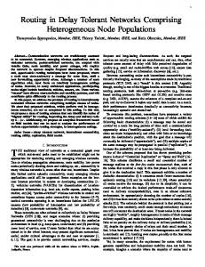
= 2 · (1 + p)log2+2p N = 2 · N log2+2p (1+p) So, min CW P DF < CW P DF (n) = 2 · N log2+2p (1+p) = O(N log2+2p (1+p) ). Since p ∈ (0, 1), log2+2p (1 + p) < So,

1 2

(see Fig. 1).

√ 2 · N log2+2p (1+p) < 2 N = min CW DF . Therefore,

Taylor & Francis and I.T. Consultant

8

0.5

f(p)=log(1+p)/log(2+2p)

0.4

f(p)

0.3 0.2 0.1 0 0

0.1 0.2 0.3 0.4 0.5 0.6 0.7 0.8 0.9

1

p

Figure 1. Curve of f (p)

min CW P DF < min CW DF Hence we see that if p ∈ (0, 1), probability delegation forwarding can further reduce the number of copies.

4.3

Cost of TPDF

In the TPDF algorithm, if a node meets a higher quality node which makes xjk −τik > T H, then it will forward immediately if the higher quality node does τik not have the message, which is equivalent to the DF algorithm; otherwise, if the quality is not that high but still higher than the node’s level, forward or not will depend on the PDF algorithm. Therefore, there are two cases here. We assume the probability of picking the DF algorithm is t(0 ≤ t ≤ 1) according to the threshold. So the probability of picking the PDF algorithm is (1 − t). Since nodes meet according to rates that are independent of node quality, the node is equally likely to meet a node with any particular quality value, E[Gn ] = 2gn still holds. We define the set B = {i|xi ≥ 1 − 2gn } as the target set, and the subtree with all the nodes whose gap < 2gn as the target-stopped tree. Therefore, the total number of copies generated can be calculated as:

CT P DF (n) = [t · 2 + (1 − t) · (1 + p)]n +

Ng 2n

In the worst case, g = 1. So,

CT P DF (n) ≤ CW T P DF = [t · 2 + (1 − t) · (1 + p)]n +

N N = [1 + t + p − tp]n + n (3) 2n 2

In Eq. (3), if t = 0, CW T P DF (n) = (1 + p)n + 2Nn = CW P DF , which is the worst case of PDF. However, if t = 1, CW T P DF (n) = 2n + 2Nn = CW DF , which is the worst case of DF. The minimum value min CT P DF of CT P DF (n) can be obtained by making its derivative equal to 0. ′ n −n ln 2 = 0 CW T P DF (n) = [1 + t + p − tp] ln[1 + t + p − tp] − N · 2

Parallel, Emergent and Distributed Systems

9

So, n = log[2+2t+2p−2tp]

N ln 2 ln[1 + t + p − tp]

Therefore,

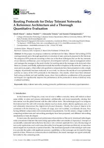
min CW T P DF = [1 + t + p − tp]log[2+2t+2p−2tp] N ln 2/ ln[1+t+p−tp] + =

30

2

log[2+2t+2p−2tp] [1+t+p−tp]

+

30

N=50 N=100 N=150 N=200

20

15

N N ln 2 ln[1+t+p−tp]

log[2+2t+2p−2tp] 2

N=50 N=100 N=150 N=200

25

f(t)

25

f(t)

N ln 2 ln[1 + t + p − tp]

N log[2+2t+2p−2tp] N ln 2/ ln[1+t+p−tp]

20

15

10

10 0

0.1 0.2 0.3 0.4 0.5 0.6 0.7 0.8 0.9 t

(a) p = 80%

1

0

0.1 0.2 0.3 0.4 0.5 0.6 0.7 0.8 0.9

1

t

(b) p = 90%

Figure 2. The curves of f (t) = min CW T P DF with different N and p

We can see that for a particular probability p, min CW T P DF is a function of t. So we denote min CW T P DF = f (t) and draw the curve of the function. If we set p = 80% and 90% and N = 50, 100, 150 and 200 respectively, as shown in Figures 2(a) and 2(b), f (t) is a monotonically increasing function. When t = 0, it is the case of P DF and when t = 1, it is DF . Therefore, the number of copies of TPDF satisfies: min CW P DF ≤ min CW T P DF ≤ min CW DF

5.

Simulations

In this section, we conduct simulations to compare the performance of DF, PDF and TPDF. We use real traces posted on [1]. The data sets consist of contact traces between short-range Bluetooth enabled devices (iMotes [4]) carried by individuals in conference environments, namely Content 2006 and Infocom 2006. In short, we call them Content trace and Info trace. In the simulations, we use three metrics as follows. • Delivery Ratio: it is defined as the fraction of generated messages that are correctly delivered to the final destination within a given time period. • Latency: it is the time between when a message is generated and when it is received. Minimizing latency lowers the time messages spend in the network, reducing contention for resources. So lowering latency indirectly improves delivery ratio.

Taylor & Francis and I.T. Consultant

10 102

100

DestFreq DestLastContact Freq LastContact

95

Delivery ratio (%)

101

Delivery ratio (%)

100

DestFreq DestLastContact Freq LastContact

99 98 97

90 85 80 75 70 65

96

60 80

85

90

95

100

80

85

Probability (%)

(a) Delivery ratio with full observation time 120k

25k

100

DestFreq DestLastContact Freq LastContact

20k

Latency

Latency

80k

95

(b) Delivery ratio with half observation time

DestFreq DestLastContact Freq LastContact

100k

90 Probability (%)

60k

15k 10k

40k 5k

20k 0

0 80

85

90

95

100

80

85

Probability (%)

DestFreq DestLastContact Freq LastContact

98

95

100

(d) Delivery latency with half observation time # of copies/DF’s # of copies (%)

# of copies/DF’s # of copies

(c) Delivery latency with full observation time 100

90 Probability (%)

96 94 92 90

DestFreq DestLastContact Freq LastContact

100 98 96 94 92 90

80

85

90

95

100

Probability (%)

(e) Ratio of PDF’s and DF’s copies with full observation time

80

85

90

95

100

Probability (%)

(f) Ratio of PDF’s and DF’s copies with half observation time

Figure 3. Comparison of DF and PDF using Content trace

• Copies: it is the number of copies of a message that a protocol generates in routing. It is an approximate measure of the computational resources required, as there is some processing required for each message. Also it is also an approximate measure of power consumption, bandwidth and buffer usages as more copies will use more of these resources. This is what we call cost in the paper. The quality of each node in DF and PDF can be decided using different forwarding algorithms as follows: • Frequency (Freq) [6]: Node ui forwards mk to node uj if uj has more total contacts with all other nodes than does ui . This algorithm is destination independent. • Last Contact (LastContact) [7]: Node ui forwards mk to node uj if uj has contacted any node more recently than has ui . This algorithm is destination independent. Destination Frequency (DestFreq) [7] : Node ui forwards mk to node uj if uj • has contacted mk ’s destination more often than has ui . • Destination Last Contact (DestLastContact) [5]: Node ui forwards mk to node uj if uj has contacted mk ’s destination more recently than has ui .

Parallel, Emergent and Distributed Systems 102

100

DestFreq DestLastContact Freq LastContact

100

Delivery ratio (%)

Delivery ratio (%)

102

DestFreq DestLastContact Freq LastContact

101

99 98 97

98 96 94 92

96 95

90 80

85

90

95

100

80

85

Probability (%)

25k

95

100

(b) Delivery ratio with half observation time 16k

DestFreq DestLastContact Freq LastContact

20k

90 Probability (%)

(a) Delivery ratio with full observation time

DestFreq DestLastContact Freq LastContact

14k 12k

15k

Latency

Latency

11

10k

10k 8k 6k 4k

5k

2k 0

0 80

85

90

95

100

80

85

Probability (%)

DestFreq DestLastContact Freq LastContact

98

95

100

(d) Delivery latency with half observation time # of copies/DF’s # of copies (%)

# of copies/DF’s # of copies

(c) Delivery latency with full observation time 100

90 Probability (%)

96 94 92 90

DestFreq DestLastContact Freq LastContact

100 98 96 94 92 90

80

85

90

95

100

Probability (%)

(e) Ratio of PDF’s and DF’s copies with full observation time

80

85

90

95

100

Probability (%)

(f) Ratio of PDF’s and DF’s copies with half observation time

Figure 4. Comparison of DF and PDF using Info trace

5.1

Comparison of DF and PDF

We first compare DF and PDF. Actually DF can be treated as a special case of PDF with a probability of 100%. So in the simulations, the results for probability 100% are actually for algorithm DF and the results for probabilities less than 100% are for PDF algorithm with different probabilities. For each of the two traces in the data sets, it has a start time and an end time. If we consider the whole lifespan of each trace, it is called the observation with full time. If we just observe a trace in half time, it is the observation with half time. The purpose to vary the length of the observation time is to see the performance of the algorithms in different time duration. We randomly generate a source and a destination. We try different probabilities starting from 80% to 100% with an increase step of 5%. We start probability from 80% because we want to save cost but at the same time, we do not want to affect delivery ratio too much. Obviously, if the probability is very small, the delivery ratio will be low during the observation time. For each source and destination pair, under a certain probability, we use all the forwarding algorithms above on both traces. We record delivery ratio, latency and the number of copies used for each set of data. The process is repeated for

Taylor & Francis and I.T. Consultant

12

50k

Freq

Latency

48k 46k 44k 42k 40k 80

85

90

95

100

Probability (%)

Figure 5. Latency of the Frequency algorithm using Content trace with full observation time

10, 000 pairs of randomly generated source and destination pairs. The results are averaged and shown in figures. Fig. 3 and 4 show the comparison of DF and PDF using the Content trace and Info trace respectively. In each trace, the three subfigures on the left column show the delivery ratio, latency and ratio of PDF’s and DF’s copies with full observation time, while the three subfigures on the right column present delivery ratio, latency and ratio of PDF’s and DF’s copies with half observation time. From the results in both traces shown in Fig. 3(a), 3(b), 4(a) and 4(b), we can see that if we use a probability above 80%, the curves in the delivery ratio are almost flat. That means, PDF has similar delivery ratio as that in DF as long as p is not too small. However, there is a slight increase in delivery latency. If we look at the Frequency algorithm using Content trace with full observation time specifically (in Fig. 3(c)) and enlarge its latency graph as in Fig. 5, we can see that DF (with probability 100% in the figure) has the lowest latency, and with the decrease of probability, the latency increases. In other words, the latency can be increased with the decrease of probability. For the number of copies, we know that DF uses the most number of copies from the analysis. Suppose the number of copies used by DF is CDF and the number DF of copies used by PDF with probability p is CP DF , we calculate ratio CCPDF . Since DF is the baseline, its ratio is 100%. As the results of both traces in Fig. 3(e), 3(f), 4(e) and 4(f) show, more and more copies can be saved with the decrease of probability. This matches our analysis in the previous section.

5.2

Comparison of DF, PDF and TPDF

Next we compare TPDF, PDF and DF. DF is PDF with a probability of 100% and PDF is TPDF without the threshold. In our simulations, we set T H to be 0.05, 0.1, 0.25 and 0.5, and the probability to be 80% for the Content trace and 85% for the Info trace. We use full observation time for the comparison of the three. We still look at the three metrics: delivery ratio, latency and number of copies. For the delivery ratio, we try Freq, LastContact, DestFreq and DestLastContact algorithms using both traces. The results are shown in Fig. 6(a) and 6(b). From the figures, the delivery ratios of DF and TPDF with T H = 0.05, 0.1, 0.25 and 0.5 are almost the same, and PDF’s is close to them. For the delivery latency, to show clearly, we just use Freq and DestLastContact algorithms as examples. In the Freq algorithm, we set the probability to be 80% and use the Content trace while in the DestLastContact algorithm, we set the probability to be 85% and use the Info trace. The results are shown in Fig. 6(c)

Parallel, Emergent and Distributed Systems

Delivery ratio (%)

101

102

DestFreq DestLastContact Freq LastContact

101.5 101

Delivery ratio (%)

102 101.5

100.5 100 99.5 99

100 99.5 99 98.5

TH=0.05

0.1

0.25

0.5

98 DF

PDF

Different thresholds

TH=0.05

0.1

0.25

0.5

PDF

Different thresholds

(a) Delivery ratio using Content trace with full observation time (p = 80%) 50k

DestFreq DestLastContact Freq LastContact

100.5

98.5 98 DF

13

(b) Delivery ratio using Info trace with full observation time (p = 85%) 20.8k

Freq

DestLastContact

20.7k 20.6k

46k

20.5k

Latency

Latency

48k

44k

20.4k 20.3k 20.2k

42k

20.1k 40k DF

TH=0.05

0.1

0.25

0.5

20.0k DF

PDF

Different thresholds

101

Freq

99 98 97 96 95 94 93 92 DF

TH=0.05

0.1

0.25

0.25

0.5

PDF

(d) Latency of DestLastContact algorithm using Info trace with full observation time (p = 85%) # of copies/DF’s # of copies

# of copies/DF’s # of copies

100

0.1

Different thresholds

(c) Latency of Freq algorithm using Content trace with full observation time (p = 80%) 101

TH=0.05

0.5

PDF

Different thresholds

(e) Ratio of Freq’s and DF’s copies using Content trace with full observation time (p = 80%)

DestLastContact

100 99 98 97 96 95 DF

TH=0.05

0.1

0.25

0.5

PDF

Different thresholds

(f) Ratio of DestLastContact’s and DF’s copies using Info trace with full observation time (p = 85%)

Figure 6. Comparison of TPDF, PDF and DF

and 6(d). In both figures, PDF has the highest latency and DF has the lowest. TPDF with T H = 0.05, 0.1, 0.25 and 0.5 can close the latency gap between PDF and DF. For the number of copies, again we use Freq and DestLastContact algorithms with the same setting. We use DF’s copy number CDF as the baseline and calculate . The results in Fig. 6(e) and 6(f) show that DF has the most ratio CotherCalgorithm DF number of copies and PDF has the least. TPDF with some threshold has a copy number between the two. This also confirms our analysis result in the previous section. From the results we know that DF, PDF and TPDF have similar delivery ratio. And the selection of a good threshold T H is important to saving more copies at a cost of slight increase in latency. For example, in the Freq algorithm as shown in Fig. 6(c) and 6(e), setting T H = 0.10 can decrease the number of copies by 5.9% from PDF at an expense of increasing latency by 1.7% from DF. And in the DestLastContact algorithm as shown in Fig. 6(d) and 6(f), setting T H = 0.05 can

REFERENCES

14

bring down the number of copies by 3.45% from PDF at a cost of increasing latency by only 0.28% from DF.

6.

Conclusion

In this paper, we enhanced the delegation forwarding (DF) scheme by putting forward a probability delegation forwarding (PDF) scheme and a threshold-based probability delegation forwarding (TPDF) scheme. PDF improves DF in reducing message copies by inserting a probability to decide whether to forward or not whereas TPDF combines DF and PDF by introducing a threshold T H. Analysis showed that the cost of PDF is less than that of DF and the cost of TPDF is between the two. Simulations demonstrated that both PDF and TPDF can achieve similar delivery ratio as the DF scheme if p is not too small. The delivery latency in PDF increases a little compared with DF. But that increase can be reduced by the TPDF scheme. If a threshold is set properly, TPDF can achieve similar latency as DF at a lower cost.

Acknowledgments

This research was supported in part by NSF grants CNS 0835834, CNS 0531410 and CNS 0626240.

References [1] CRAWDAD: A community resource for archiving wireless data at dartmoutn. Available at http://crawdad.cs.dartmouth.edu. [2] X. C. Chen and A. L. Murphy, Enabling Disconnected Transitive Communication in Mobile Ad Hoc Networks, Proc. of the Workshop on Principles of Mobile Computing (POMC), August, 2001, pp. 21-27. [3] A. Broder, A. Kirsh, R. Kumar, M. Mitzenmacher, E. Upfal and S. Vassilvitskii, The hiring problem and lake wobegon strategies, Proc. of ACM-SIAM SODA, 2008. [4] A. Chaintreau, P. Hui, J. Crowcroft, C. Diot, R. Gass, and J. Scott, Impact of human mobility on opportunistic forwarding algorithms, IEEE Transaction on Mobile Computing 6, 6 (2007), p. 606-620. [5] H. Dubois-Ferriere, M. Grossglauser, and M. Vetterli, Age matters: efficient route discovery in mobile ad hoc networks using encounter ages, Proc. of ACM MobiHoc, 2003. [6] V. Erramilli, A. Chaintreau, M. Crovella, and C. Diot, Diversity of forwarding paths in pocket switched networks, Proc. of ACM/SIGCOMM IMC, 2007, p. 41-50. [7] V. Erramilli, M. Crovella, A. Chaintreau and C. Diot, Delegation Forwarding, Proc. of MobiHoc, May 2008, p. 251-259. [8] J. Ghosh, S. J. Philip, and C. Qiao, Sociological orbit aware location approximation and routing (SOLAR) in MANET, Proc. of ACM MobiHoc, 2005. [9] S. Jain, K. Fall, and R. Patra, Routing in a delay tolerant network, Proc. of ACM SIGCOMM, 2004. [10] E. P. C. Jones and P. A. S. Ward, Routing Strategies for Delay-Tolerant Networks, Proc. of ACM SIGCOMM, 2004. [11] P. Juang, H. Oki, Y. Wang, M. Martonosi, L. S. Peh, and D. Rubenstein, Energy-efficient computing for wildlife tracking: design tradesoffs and early experiences with zebranet, Proc. of ASPLOS-X, 2002, pp. 96-107. [12] J. Leguay, T. Friedman, and V. Conan, DTN routing in a mobility pattern space, Proc. of ACM SIGCOMM Workshop on Delay-Tolerant Networking, 2005. [13] A. Lindgren, A. Doria, and O. Schelen, Probabilistic routing in intermittently connected networks, Lecture Notes in Computer Science, 3126:239-254, August 2004. [14] C. Liu and J. Wu, Routing in a Cyclic MobiSpace, Proc. of the 9th ACM International Symposium on Mobile Ad Hoc Networking and Computing (MobiHoc), 2008. [15] C. Liu and J. Wu, An Optimal Probabilistically Forwarding Protocol in Delay Tolerant Networks, Proc. of 10th ACM International Symposiumon Mobile Ad Hoc Networking and Computing (MobiHoc), 2009. [16] S. Merugu, M. Ammar, and E. Zegura, Routing in space and time in network with predictable mobility, Technical report: GIT-CC-04-07, College of Computing, Georgia Tech, 2004. [17] T. Spyropoulos, K. Psounis, and C. S. Raghavendra, Single-copy routing in intermittently connected mobile networks, Proc. of IEEE Secon, 2004.

REFERENCES

15

[18] T. Spyropoulos, K. Psounis, and C. S. Raghavendra, Spray and Focus: Efficient Mobility-Assisted Routing for Heterogeneous and Correlated Mobility, Proc. of the Fifth IEEE International Conference on Pervasive Computing and Communications Workships (PERCOMW) 2007, 2007. [19] M. M. B. Tariq, M. Ammar, and E. Zegura, Message ferry route design for sparse ad hoc networks with mobile nodes, Proc. of ACM MobiHoc, 2005. [20] J. Wu, S. Yang, and F. Dai, Logarithmic store-carry-forward routing in mobile ad hoc networks, IEEE Transactions on Parallel and Distributed Systems, 18(6), June 2007. [21] A. Vahdat, and D. Becker, Epidemic routing for partially connected ad hoc networks, Techical Report CS-200006, Duke University, 2000.