or positive programs, whose answer set semantics can be used to defined the semantics of the original programs. ..... The key idea that makes this possible is the general- ization of the ...... person(P), table(T), not not at(P, T) not at(P, T) ...
arXiv:cs/0605038v1 [cs.SE] 9 May 2006
An Unfolding-Based Semantics for Logic Programming with Aggregates Tran Cao Son, Enrico Pontelli, Islam Elkabani Computer Science Department New Mexico State University Las Cruces, NM 88003, USA {tson,epontell,ielkaban}@cs.nmsu.edu
Abstract The paper presents two equivalent definitions of answer sets for logic programs with aggregates. These definitions build on the notion of unfolding of aggregates, and they are aimed at creating methodologies to translate logic programs with aggregates to normal logic programs or positive programs, whose answer set semantics can be used to defined the semantics of the original programs. The first definition provides an alternative view of the semantics for logic programming with aggregates described in [32, 34]. In particular, the unfolding employed by the first definition in this paper coincides with the translation of programs with aggregates into normal logic programs described in [33]. This indicates that the approach proposed in this paper captures the same meaning as the semantics discussed in [32, 34]. The second definition is similar to the traditional answer set definition for normal logic programs, in that, given a logic program with aggregates and an interpretation, the unfolding process produces a positive program. The paper shows how this definition can be extended to consider aggregates in the head of the rules. These two approaches are very intuitive, general, and do not impose any syntactic restrictions on the use of aggregates, including support for use of aggregates as heads of program rules. The proposed views of logic programming with aggregates are simple and coincide with the ultimate stable model semantics [32, 34], and with other semantic characterizations for large classes of program (e.g., programs with monotone aggregates and programs that are aggregate-stratified). Moreover, it can be directly employed to support an implementation using available answer set solvers. The paper describes a system, called ASPA , that is capable of computing answer sets of programs with arbitrary (e.g., recursively defined) aggregates. The paper also presents an experimental comparison of ASPA with another system for computing answer sets of programs with aggregates, DLVA .
1
Contents 1 Background and Motivation
3
2 A Logic Programming Language with Aggregates
5
3 Aggregate Solutions and Unfolding 3.1 Solutions of Aggregates . . . . . . 3.2 ASPA Answer Sets . . . . . . . . . 3.3 Properties of ASPA -Answer Sets . 3.4 Implementation . . . . . . . . . . . 3.4.1 Computing the Solutions . 3.4.2 The ASPA System . . . . . 3.4.3 Some Experimental Results
Semantics . . . . . . . . . . . . . . . . . . . . . . . . . . . . . . . . . . . . . . . . . . . . . . . . .
. . . . . . .
. . . . . . .
. . . . . . .
. . . . . . .
. . . . . . .
. . . . . . .
. . . . . . .
. . . . . . .
. . . . . . .
. . . . . . .
. . . . . . .
. . . . . . .
. . . . . . .
. . . . . . .
. . . . . . .
. . . . . . .
. . . . . . .
. . . . . . .
. . . . . . .
. . . . . . .
. . . . . . .
. . . . . . .
. . . . . . .
. . . . . . .
. . . . . . .
. . . . . . .
. . . . . . .
. . . . . . .
. . . . . . .
. . . . . . .
. . . . . . .
8 8 10 12 14 14 16 17
4 An Alternative Semantical Characterization 20 4.1 Unfolding with respect to an Interpretation . . . . . . . . . . . . . . . . . . . . . . . . . . . . . . . . . 20 4.2 Aggregates in the Head of Rules . . . . . . . . . . . . . . . . . . . . . . . . . . . . . . . . . . . . . . . 23 5 Related Work 5.1 Pelov’s Approximation Semantics for Logic Program with Aggregates 5.2 ASPA -Answer Sets and Minimality Condition . . . . . . . . . . . . . . 5.3 Logic Programs with Abstract Constraint Atoms . . . . . . . . . . . . 5.4 Answer Sets for Propositional Theories . . . . . . . . . . . . . . . . . . 5.5 Logic Programs with Weight Constraints . . . . . . . . . . . . . . . . . 5.6 Stratified Programs . . . . . . . . . . . . . . . . . . . . . . . . . . . . . 5.7 Monotone Programs . . . . . . . . . . . . . . . . . . . . . . . . . . . . 5.8 Other Proposals . . . . . . . . . . . . . . . . . . . . . . . . . . . . . .
. . . . . . . .
. . . . . . . .
. . . . . . . .
. . . . . . . .
. . . . . . . .
. . . . . . . .
. . . . . . . .
. . . . . . . .
. . . . . . . .
. . . . . . . .
. . . . . . . .
. . . . . . . .
. . . . . . . .
. . . . . . . .
. . . . . . . .
. . . . . . . .
. . . . . . . .
. . . . . . . .
25 25 26 28 30 31 33 34 36
6 Discussions 36 6.1 A Limitation of the Unfolding Transformation . . . . . . . . . . . . . . . . . . . . . . . . . . . . . . . . 36 6.2 Computational Complexity . . . . . . . . . . . . . . . . . . . . . . . . . . . . . . . . . . . . . . . . . . 37 7 Conclusions and Future Work
37
2
1
Background and Motivation
The handling of aggregates in Logic Programming (LP) has been the subject of intense studies in the late 80’s and early 90’s [20, 28, 36, 42, 43]. Most of these proposals focused on the theoretical foundations and computational properties of aggregate functions in LP. The recent development of the answer set programming paradigm, whose underlying theoretical foundation is the answer set semantics [14], has renewed the interest in the treatment of aggregates in LP, and led to a number of new proposals [5, 6, 10, 12, 13, 16, 26, 32–34, 39]. Unlike many of the earlier proposals, these new efforts provide a sensible semantics for programs that makes a general use of aggregates, including the presence of recursion through the aggregates and the ability to use non-monotone aggregate functions. Most of these new efforts build on the spirit of answer set semantics for LP, and some have found their way in concrete implementations. For example, the current release (built BEN/Jan 13 2006)1 of DLVA handles aggregate-stratified programs [5], and the system described in [10] supports recursive aggregates according to the semantics described in [20]. A prototype of the ASET-Prolog system, capable of supporting recursive aggregates, has also been developed [18]. Answer set semantics for LP [14] has been one of the most widely adopted semantics for normal logic programs—i.e., logic programs that allow negation as failure in the body of the rules. It is a natural extension of the minimal model semantics of positive logic programs to the case of normal logic programs. Answer set semantics provides the theoretical foundation for the recently emerging programming paradigm called answer set programming [23, 27, 29] which has proved to be useful in several applications [1, 2, 23]. A set of atoms S is an answer set of the program P if S is the minimal model of the positive program P S (the reduct of P with respect to S), obtained by (i) removing from P all the rules whose body contains a negation as failure literal not b which is false in S (i.e., b ∈ S); and (ii) removing all the negation as failure literals from the remaining rules. The above transformation is often referred to as the Gelfond-Lifschitz transformation. This definition of answer sets satisfies several important properties. In particular, answer sets are (Pr1 ) closed, i.e., if an answer set satisfies the body of a rule r then it also satisfies its head; (Pr2 ) supported—i.e., for each member p of an answer set S there exists a rule r ∈ P such that p is the head of the rule and the body of r is true in S; (Pr3 ) minimal—i.e., no proper subset of an answer set is also an answer set. It should be emphasized that the properties (Pr1 )-(Pr3 ) are necessary but not sufficient conditions for a set S to be an answer set of a program P . For example, the set {p} is not an answer set of the program {p ← p, q ← not p}, even though it satisfies the three properties. Nevertheless, these properties constitute the main principles that guided several extensions of the answer set semantics to different classes of logic programs, such as extended and disjunctive logic programs [15], programs with weight constraint rules [30], and programs with aggregates (e.g., [5, 20]). It should also be mentioned that, for certain classes of logic programs (e.g., programs with weight 1
http://www.dbai.tuwien.ac.at/proj/dlv
3
constraints and choice rules [30] or with nested expressions [24]), (Pr3 ) is not satisfied. It is, however, generally accepted that (Pr1 ) and (Pr2 ) must be satisfied by any answer set definition for any extension of logic programs. As evident from the literature, a straightforward extension of the Gelfond-Lifschitz transformation to programs with aggregates leads to the loss of some of the properties (Pr1 )-(Pr3 ) (e.g., presence of non-minimal answer sets [20]). Sufficient conditions, that characterize classes of programs with aggregates for which the properties (Pr1 )-(Pr3 ) of answer sets hold, have been investigated, such as aggregate-stratification and monotonicity (e.g., [28]). Alternatively, researchers have either accepted the loss of some of the properties (Pr1 )-(Pr3 ) (e.g., acceptance of non-minimal answer sets [10, 16, 20]) or have explicitly introduced minimality or analogous properties as requirements in the definition of answer sets for programs with aggregates (e.g., [12, 13]). The various approaches for defining answer set semantics for logic programs with arbitrary aggregates differ from each other in both the languages that are considered and in the treatment of aggregates. Some proposals accept languages in which aggregates, or atoms representing aggregates (e.g., the weight constraints in Smodels-notation), are allowed to occur in the head of programs’ rules or as facts in [13, 26, 30], while this has been disallowed in other proposals [5, 6, 10, 12, 16, 32, 34]. The advantage of allowing aggregates in the head can be seen in the use of choice rules and weight constraints in generate and test programs. Allowing aggregates in the head can make the encoding of a problem significantly more declarative and compact. Similarly, some proposals do not consider negation-as-failure literals with aggregates [10, 16]. The recent approaches for defining answer sets for logic programs with arbitrary aggregates can be roughly divided into three different groups. The first group can be viewed as a straightforward generalization of the work in [14], by treating aggregates in the same way as negation-as-failure literals. Belonging to this group are the proposals in [10, 16, 20]. A limitation of this approach is that it leads to the acceptance of unintuitive answer sets, in presence of recursion through aggregates. Another line of work is to replace aggregates with equivalent formulae, according to some notion of equivalence, and to reduce programs with aggregates to programs for which the semantics has already been defined [10, 13, 33]. A third direction is to make use of novel semantic constructions [6, 12, 26, 32, 34, 39]. The objective of this paper is to investigate an alternative characterization of the semantics of logic programs with unrestricted use of aggregates. In this context, aggregates are simply viewed as a syntactic sugar, representing a collection of constraints on the admissible interpretations. The proposed characterization is designed to maintain the positive properties of the most recent proposals developed to address this problem (e.g., [12, 13, 32]), and to meet the following requirements: • It should apply to programs with arbitrary aggregates (e.g., no syntactic restrictions in the use of aggregates as well as no restrictions on the types of aggregates that can be used). In particular, we wish the approach to naturally support aggregates as facts and as heads of rules. • It should be as intuitive as the traditional answer set semantics, and it should extend traditional answer set semantics—i.e., it should behave as traditional answer set semantics for programs without aggregates. It should also naturally satisfy the basic properties (Pr1 )-(Pr3 ) of answer sets. • It should offer ways to implement the semantic characterization by integrating, with minimal modifications, the definition in state-of-the-art answer set solvers, such as Smodels [31], 4
dlv [9], Cmodels [21], ASSAT [22], etc. In particular, it should require little more than the addition of a module to determine the “solutions” of an aggregate,2 without substantial modifications of the mechanisms to compute answer sets. We achieve these objectives by defining a transformation, called unfolding, from logic programs with aggregates to normal logic programs. The key idea that makes this possible is the generalization of the supportedness property of answer sets to the case of aggregates. More precisely, our transformation ensures that, if an aggregate atom is satisfied by a model M , then M supports at least one of its solutions. Solutions of aggregates can be precomputed, and an answer set solver for LP with aggregates can be implemented using standard answer set solvers. The notion of unfolding has been widely used in various areas of logic programming (e.g., [35, 37, 41]). The inspiration for the approach used in handling aggregates in this paper comes from the methodology proposed in various works on constructive negation (e.g., [4, 7, 40])—in particular, from the idea of unfolding intensional sets into sets of solutions, employed to handle intensional sets in [3, 7]. The approach developed in this paper is the continuation and improvement of the approach in [10]. It offers an alternative view of the semantics for LP with aggregates developed in [32]. In particular, the two characterizations provide the same meaning to program with aggregates, although our approach does not require the use of approximation theory. We provide two ways of using unfolding. The first is similar to the notion of transformation explored in [33]. The second is closer to the spirit of the original definition of answer sets [14], and it allows us to naturally handle more general use of aggregates (e.g., aggregates in the heads). The characterization proposed in this paper also captures the same meaning as the proposals in [12, 13, 26] for large classes of programs (e.g., stratified programs and programs with monotone aggregates). Observe that, in this work, we do not directly address the problem of negated aggregates. This problem can be tackled in different ways (e.g. [13, 26]). Our approach to aggregates can be easily extended to accommodate any of these approaches [38]. The rest of this paper is organized as follows. Section 2 presents the syntax of our logic programming language with aggregates. Section 3 describes the first definition of answer sets for programs with aggregates that do not allow for aggregates to occur in the head of rules. The definition is based on an unfolding transformation of programs with aggregates into normal logic programs. It also contains a discussion of properties of answer sets and describes an implementation. Section 4 introduces an alternative unfolding, which is useful for extending the use of aggregates to the head of program rules. Section 5 compares our approach with the relevant literature. Section 6 discusses some issues related to our approach to providing semantics of aggregates. Finally, Section 7 presents the conclusions and the future work.
2
A Logic Programming Language with Aggregates
Let us consider a signature ΣL = hFL ∪ FAgg , V ∪ Vl , ΠL ∪ ΠAgg i, where • FL is a collection of constants (program constants), • FAgg is a collection of unary function symbols (aggregate functions), 2
This concept is formalized later in the paper.
5
• V and Vl are denumerable collections of variables, such that V ∩ Vl = ∅, • ΠL is a collection of arbitrary predicate symbols (program predicates), and • ΠAgg is a collection of unary predicate symbols (aggregate predicates). In the rest of this paper, we will assume that Z is a subset of FL —i.e., there are distinct constants representing the integer numbers. We will refer to ΣL as the ASP signature. We will also refer to ΣP = hFP , V ∪ Vl , ΠP i as the program signature, where • FP ⊆ FL , • ΠP ⊆ ΠL , and • FP is finite. We will denote with HP the ΣP -Herbrand universe, containing the ground terms built using symbols of FP , and with BP the corresponding ΣP -Herbrand base. We will refer to an atom of the form p(t1 , . . . , tn ), where ti ∈ FP ∪V and p ∈ ΠP , as an ASP-atom. An ASP-literal is either an ASP-atom or the negation as failure (not A) of an ASP-atom. Definition 1 An extensional set has the form {t1 , . . . , tk }, where ti are terms of ΣP . An extensional multiset has the form {{t1 , . . . , tk }} where ti are (possibly repeated) terms of ΣP . Definition 2 An intensional set is of the form {X | p(X1 , . . . , Xk )} where X ∈ Vl is a variable, Xi ’s are variables or constants, {X1 , . . . , Xk } ∩ Vl = {X}, and p is a k-ary predicate in ΠP . An intensional multiset is of the form {{X | ∃Z1 , . . . , Zr . p(Y1 , . . . , Ym )}} where {Z1 , . . . , Zr , X} ⊆ Vl , Y1 , . . . , Ym are variables or constants (of FP ), {Y1 , . . . , Ym } ∩ Vl = {X, Z1 , . . . , Zr }, and X ∈ / {Z1 , . . . , Zr }. We call X and p the collected variable and the predicate of the set/multiset, respectively. Intuitively, we are collecting the values of X that satisfy the atom p(Y1 , . . . , Ym ), under the assumption that the variables Zj are locally and existentially quantified. For example, if p(X, Z) is true for X = 1, Z = 2 and X = 1, Z = 3, then the multiset {{X | ∃Z.p(X, Z)}} corresponds to {{1, 1}}. Definition 2 can be extended to allow more complex types of sets, e.g., sets collecting tuples as elements, sets with conjunctions of literals as property of the intensional construction, and intensional sets with existentially quantified variables. Observe also that the variables from Vl are used exclusively as collected or local variables in defining intensional sets or multisets, and they cannot occur anywhere else. Definition 3 An aggregate term is of the form f (s), where s is an intensional set or multiset, and f ∈ FAggr . An aggregate atom has the form p(α) where p ∈ ΠAgg and α is an aggregate term. 6
This notation for aggregate atoms is more general than the one used in some previous works, and resembles the abstract constraint atom notation presented in [26]. In our examples, we will focus on the “standard” aggregate functions and predicates, e.g., Count, Sum, Min, Max, Avg applied to sets/multisets and predicates such as =, 6=, ≤, etc. Also, for the sake of readability, we will often use a more traditional notation when dealing with the standard aggregates; e.g., instead of writing ≤7 (Sum({X |p(X)})) we will use the more common format Sum({X | p(X)}) ≤ 7. Given an aggregate atom ℓ, with k-ary collected predicate p, we denote with H(ℓ) the following set of ASP-atoms: H(ℓ) = {p(a1 , . . . , ak ) | {a1 , . . . , ak } ⊆ HP } Definition 4 An ASPA rule is an expression of the form A ← C1 , . . . , Cm , A1 , . . . , An , not B1 , . . . , not Bk
(1)
where A, A1 , . . . , An , B1 , . . . , Bk are ASP-atoms, and C1 , . . . , Cm are aggregate atoms (m ≥ 0, n ≥ 0, k ≥ 0).3 An ASPA program is a collection of ASPA rules. For an ASPA rule r of the form (1), we use the following notations: ◦ head(r) denotes the ASP-atom A, ◦ agg(r) denotes the set {C1 , . . . , Cm }, ◦ pos(r) denotes the set {A1 , . . . , An }, ◦ neg(r) denotes the set {B1 , . . . , Bk }, ◦ body(r) denotes the right hand side of the rule r. For a program P , lit(P ) denotes the set of all ASP-atoms present in P . The syntax has been defined in such a way that collected and local variables of an aggregate atom ℓ have a scope that is limited to ℓ. Thus, given an ASPA rule, it is possible to rename these variables apart, so that each aggregate atom Ci in the body of a rule makes use of different collected and local variables. Observe also that the collected and the local variables are the only occurrences of variables from Vl , and these variables will not appear in any of head(r), pos(r), and neg(r). Definition 5 Given a term (atom, literal, rule) β, we denote with f vars(β) the set of variables from V present in β. We will refer to these as the free variables of β. The entity β is ground if f vars(β) = ∅. In defining the semantics of the language, we will need to consider all possible ground instances of programs. A ground substitution θ is a set {X1 /a1 , . . . , Xk /ak }, where the Xi are distinct elements of V and the elements aj are constants from FP . Given a substitution θ and an ASP-atom (or an aggregate atom) p, the notation pθ describes the atom obtained by simultaneously replacing each occurrence of Xi (1 ≤ i ≤ k) with ai . The resulting element pθ is the instance of p w.r.t. θ. Given a rule r of the form (1) with f vars(r) = {X1 , . . . , Xn }, and given a ground substitution θ = {X1 /a1 , . . . , Xn /an }, the ground instance of r w.r.t. θ is the rule obtained from r by simultaneously replacing every occurrence of Xi (i = 1, . . . , n) in r with ai . 3
For methods to handle negated aggregate atoms, the reader is referred to [38].
7
We will denote with ground(r) the set of all the possible ground instances of a rule r that can be constructed in ΣP . For a program P , we S will denote with ground(P ) the set of all ground instances of all rules in P , i.e., ground(P ) = r∈P ground(r). Observe that a ground logic program with aggregates differs from a ground logic program, in that it might still contain some local variables, which are members of Vl , and they occur only in aggregate atoms. Example 1 Let V = {Y }, Vl = {X}, FP = {1, 2, −2}, and ΠP = {p, q}. Let r be the rule q(Y ) ← Sum({X | p(X, Y )}) ≥ 0. ground(r) will contain the following rules: q(1) ← Sum({X | p(X, 1)}) ≥ 0. q(2) ← Sum({X | p(X, 2)}) ≥ 0. q(−2) ← Sum({X | p(X, −2)}) ≥ 0. Furthermore, for the aggregate atom ℓ = Sum({X | p(X, 1)}) ≥ 0, we have that H(ℓ) = {p(1, 1), p(2, 1), p(−2, 1)}. 2
3
Aggregate Solutions and Unfolding Semantics
In this section, we develop our first characterization of the semantics of program with aggregates, based on answer sets, study some of its properties, and investigate an implementation based on the Smodels system.
3.1
Solutions of Aggregates
Let us start by developing the notion of interpretation, following the traditional structure [25]. Definition 6 (Interpretation Domain) The domain D of an interpretation is the set D = HP ∪ 2HP ∪ M(HP ), where 2HP is the set of all (finite) subsets of HP , while M(HP ) denotes the set of all finite multisets built using elements from HP . Definition 7 (Interpretation) An interpretation I is a pair hD, (·)I i, where (·)I is a function that maps ground terms to elements of D and ground atoms to truth values. The interpretation function (·)I is defined as follows: • if c is a constant, then cI = c • if s is a ground intensional set {X | q}, then sI is the set {a1 , . . . , ak } ∈ 2HP , where (q{X/b})I is true if and only if b ∈ {a1 , . . . , ak }. ¯ }, then sI is the multiset {{a1 , . . . , ak }} ∈ • if s is a ground intensional multiset {{X | ∃Z.q} M(HP ), where, for each i = 1, . . . k, there exists a ground substitution ηi for Z¯ such that ( q(ηi ∪ {X/ai }) )I is true, and no other element has such property. 8
• given an aggregate term f (s), then f (s)I is equal to f I (sI ), where f I : 2HP ∪ M(HP ) → FP • if p(a1 , . . . , ak ) is a ground ASP-atom or a ground aggregate atom, then p(a1 , . . . , ak )I is pI (aI1 , . . . , aIk ), where pI : D k → {true, f alse}. In the characterization of the aggregate functions, in this work we will mostly focus on functions that maps sets/multisets to integer numbers in Z. We will also assume that the traditional aggregate functions and predicates are interpreted in the usual manner. E.g., SUMI is the function that sums the elements of a set/multiset, and ≤I7 is the predicate that is true if its argument is an element of Z no greater than 7. Given a literal not p, its interpretation (not p)I is true (false) iff pI is false (true). For the sake of simplicity, given an atom (literal, aggregate atom) p, we will denote with I |= p the fact that pI is true. Definition 8 (Rule Satisfaction) Let I be an interpretation and r an ASPA rule. I satisfies the body of the rule (I |= body(r)) if I |= q for each q ∈ body(r). We say that I satisfies r if I |= head(r) whenever I |= body(r). Finally, we can define the concept of model of a program. Definition 9 (Model of a Program) An interpretation I is a model of a program P if M satisfies each rule r ∈ ground(P ). In the rest of this work, we will assume that the interpretation of the aggregate functions and predicates is fixed—i.e., it is the same in all the interpretations. This allows us to keep the “traditional” view of interpretations as subsets of BP [25]. Definition 10 (Minimal Model) An interpretation I is a minimal model of P if I is a model of P and there is no proper subset of I which is also a model of P . We will now present the notion of solution of an aggregate. One of the guiding principles behind this concept is the following observation. The satisfaction of an ASP-atom p is monotonic, in the sense that if I |= p and I ⊆ I ′ , then we have that I ′ |= p. This property does not hold any longer when we consider aggregate atoms. Furthermore, the truth value of an aggregate atom ℓ depends on the truth value of certain atoms belonging to H(ℓ). For example, if we consider the aggregate atom ℓ = SUM({X | p(X)}) ≤ 1 in the program with H(ℓ) = {p(1), p(2), p(−1)}, we can observe that {p(1)} |= SUM({X | p(X)}) ≤ 1 {p(1), p(2)} 6|= SUM({X | p(X)}) ≤ 1 and ℓ is true if p(2) is false or p(−1) is true. These two observations lead to the following definition. Definition 11 (Aggregate Solution) Let ℓ be a ground aggregate atom. A solution of ℓ is a pair hS1 , S2 i of disjoint subsets of H(ℓ) such that, for every interpretation I, if S1 ⊆ I and S2 ∩ I = ∅ then I |= ℓ. We will denote with SOLN (ℓ) the set of all the solutions of the aggregate atom ℓ. 9
Let S = hS1 , S2 i be the solution of an aggregate ℓ; we denote with S.p and S.n the two components S1 and S2 of the solution. Example 2 Let c be the aggregate atom Sum({X | p(X)})6=5 in a language where H(c) = {p(1), p(2), p(3)}. This aggregate atom has a total of 19 solutions of the form hS1 , S2 i such that S1 , S2 ⊆ {p(1), p(2), p(3)}, S1 ∩ S2 = ∅, and (i) either p(1) ∈ S1 ; or (ii) {p(2), p(3)} ∩ S2 6= ∅. These solutions are listed below. h{p(1)}, ∅i h{p(1)}, {p(2), p(3)}i h{p(1), p(3)}, ∅i h{p(2)}, {p(3), p(1)}i h{p(1), p(2), p(3)}, ∅i h∅, {p(1), p(2)}i h∅, {p(1), p(2), p(3)}i
h{p(1)}, {p(2)}i h{p(1), p(2)}, ∅i h{p(1), p(3)}, {p(2)}i h{p(3)}, {p(2)}i h∅, {p(2)}i h∅, {p(1), p(3)}i
h{p(1)}, {p(3)}i h{p(1), p(2)}, {p(3)}i h{p(2)}, {p(3)}i h{p(3)}, {p(2), p(1)}i h∅, {p(3)}i h∅, {p(2), p(3)}i 2
Let ℓ be an aggregate atom. The following properties hold: Observation 3.1 (i) If there is at least one interpretation I such that I |= ℓ, then SOLN(ℓ) 6= ∅. (ii) If Sℓ is a solution of ℓ then, for every set S ′ ⊆ H(ℓ) with S ′ ∩ (Sℓ .p ∪ Sℓ .n) = ∅, we have that hSℓ .p, Sℓ .n ∪ S ′ i and hSℓ .p ∪ S ′ , Sℓ .ni are also solutions of ℓ. The first property holds since the pair hI ∩ H(ℓ), H(ℓ) \ Ii is a solution of ℓ. The second property is trivial from the definition of a solution.
3.2
ASPA Answer Sets
We will now define the unfolding of an aggregate atom, of V a ground rule,Vand of a program. For simplicity, we use S (resp. not S) to denote the conjunction a∈S a (resp. b∈S not b) when S 6= ∅; ∅ (not ∅) stands for ⊤ (⊥).4 Definition 12 (Unfolding of an Aggregate Atom) Given a ground aggregate atom ℓ and a solution S ∈ SOLN(ℓ), the unfolding of ℓ w.r.t. S, denoted by ℓ(S), is S.p ∧ not S.n. Definition 13 (Unfolding of a Rule) Let r be a ground rule A ← C1 , . . . , Cm , A1 , . . . , An , not B1 , . . . , not Bk ′ where hCi im i=1 are aggregate atoms. A ground rule r is an unfolding of r if there exists a sequence of aggregate solutions SC1 , . . . , SCm such that
1. SCi is a solution of the aggregate atoms Ci (i = 1, . . . , m), 2. head(r ′ ) = head(r), S 3. pos(r ′ ) = pos(r) ∪ m i=1 SCi .p,
4
We follow the convention of denoting true with ⊤ and f alse with ⊥.
10
4. neg(r ′ ) = neg(r) ∪ 5. agg(r ′ ) = ∅.
Sm
i=1 SCi .n,
and
We say that r ′ is an unfolding of r with respect to hSCi im i=1 . The set of all possible unfoldings of a rule r is denoted by unf olding(r). For an ASPA program P , unf olding(P ) denotes the set of the unfoldings of the rules in ground(P ). It is easy to see that unf olding(P ) is a normal logic program. The answer sets of ASPA programs are defined as follows. Definition 14 A set of atoms M is an ASPA -answer set of P iff M is an answer set of unf olding(P ). Example 3 Let P1 be the program:5 p(a) ← Count({X | p(X)}) > 0 p(b) ← not q q ← not p(b) The aggregate atom Count({X | p(X)}) > 0 has five aggregate solutions: h{p(a)}, ∅i
h{p(b)}, ∅i
h{p(a), p(b)}, ∅i h{p(a)}, {p(b)}i
h{p(b)}, {p(a)}i
The unfolding of P1 is the program p(a) p(a) p(b) p(a)
← ← ← ←
p(a) ← p(b) p(a) ← p(a), not p(b) q ← not p(b)
p(a) p(a), p(b) not q p(b), not p(a)
M1 = {q} and M2 = {p(b), p(a)} are the two answer sets of unf olding(P1 ), thus ASPA -answer sets of P1 . 2 Example 4 Let P2 be the program p(1) p(2) p(3) p(5) q
← ← ← ← q ← Sum({X | p(X)}) > 10
The only aggregate solution of Sum({X | p(X)}) > 10 is h{p(1), p(2), p(3), p(5)}, ∅i and unf olding(P2 ) contains: p(1) ← p(2) ← p(3) ← p(5) ← q q ← p(1), p(2), p(3), p(5) which has M1 = {p(1), p(2), p(3)} as its only answer set. Thus, M1 is the only ASPA -answer set of P2 . 2 5
We would like to thank Vladimir Lifschitz for suggesting this example.
11
The next program with aggregates does not have answer sets, even though it does not contain any negation as failure literals. Example 5 Consider the program P3 : p(2) ← p(1) ← Min({X | p(X)}) ≥ 2 The unique aggregate solution of the aggregate atom Min({X | p(X)}) ≥ 2 with respect to BP3 = {p(1), p(2)} is h{p(2)}, {p(1)}i. The unfolding of P3 consists of the two rules: p(2) ← p(1) ← p(2), not p(1) and it does not have any answer sets. As such, P3 does not have any ASPA -answer sets.
2
Observe that, in creating unf olding(P ), we use every solution of c in SOLN(c). Since the number of solutions of an aggregate atom can be exponential in the size of the Herbrand base, the size of unf olding(P ) can be exponential in the size of P . Fortunately, as we will show later (Theorem 2), this process can be simplified by considering only minimal solutions of each aggregate atom (Definition 16). In practice, for most common uses of aggregates, we have observed a small number of elements in the minimal solution set (typically linear or quadratic in the extension of the predicate used in the intensional set).
3.3
Properties of ASPA -Answer Sets
It is easy to see that the notion of ASPA -answer sets extends the notion of answer sets of normal logic programs. Indeed, if P does not contain aggregate atoms, then unf olding(P ) = ground(P ). Thus, for a program without aggregates P , M is an ASPA -answer set of P if and only if M is an answer set of P with respect to the Gelfond-Lifschitz definition of answer sets. We will now show that ASPA -answer sets satisfies the same properties of minimality, closedness, and supportedness as answer sets for normal logic programs. Lemma 1 Every model of unf olding(P ) is a model of P . Proof. Let M be a model of unf olding(P ), and let us consider a rule r ∈ ground(P ) such that M satisfies the body of r. This implies that there exists a sequence of solutions hSc ic∈agg(r) for the aggregate atoms occurring in r, such that Sc ∈ SOLN (c), Sc .p ⊆ M , and Sc .n ∩ M = ∅. Let r ′ be the unfolding of r with respect to hSc ic∈agg(r) . We have that pos(r ′ ) ⊆ M and neg(r ′ ) ∩ M = ∅. In other words, M satisfies the body of r ′ ∈ unf olding(P ). This implies that head(r ′ ) ∈ M , i.e., head(r) ∈ M . 2 Lemma 2 Every model of P is a model of unf olding(P ). Proof. Let M be a model of P , and let us consider a rule r ′ ∈ unf olding(P ) such that M satisfies the body of r ′ . Since r ′ ∈ unf olding(P ), there exists r ∈ ground(P ) and a sequence of aggregate solutions hSc ic∈agg(r) for the aggregate atoms in r such that M satisfies Sc .p∧not Sc .n (for c ∈ agg(r)) and r ′ is the unfolding of r with respect to hSc ic∈agg(r) . This means that pos(r) ⊆ M , neg(r) ∩ M = ∅, and M |= c for c ∈ agg(r). In other words, M satisfies body(r). Since M is a model of ground(P ), we have that head(r) ∈ M , which means that head(r ′ ) ∈ M . 2 12
Theorem 1 Let P be a program with aggregates and M be an ASPA -answer set of P . Then, M is closed, supported, and a minimal model of ground(P ). Proof. Since M is an ASPA -answer set of P , Lemma 1 implies that M is a model of ground(P ). Minimality of M follows from Lemma 2 and from the fact that M is a minimal model of unf olding(P ). Closedness is immediate from Lemma 1. Supportedness can be derived from the fact that each atom p in M is supported by M (w.r.t. unf olding(P )) since M is an answer set of unf olding(P ). Thus, if p were not supported by M w.r.t. ground(P ), then this would mean that no rule in unf olding(P ) supports p, which would contradict the fact that M is an answer set of unf olding(P ). 2 Observe that the converse of the above theorem does not hold, as illustrated by the following example. Example 6 Let P4 be the program p(1) p(2) q q
← ← q ← Sum({X | p(X)}) ≥ 2 ← Sum({X | p(X)}) < 2
It is easy to see that M = {p(1), p(2), q} is a minimal model of this ground program—i.e., M is a minimal set of atoms, closed under the rules of ground(P4 ) and each atom of M is supported by a rule of ground(P4 ). On the other hand, unf olding(P4 ) consists of the following rules p(1) p(2) q q q
← ← ← ← ←
q p(2) p(1), not p(2) not p(2)
q ← p(1), p(2) q ← p(2), not p(1) q ← not p(1), not p(2)
M is not an answer set of unf olding(P4 ). We can easily check that this program does not have an answer set. Thus, P4 does not have an answer set according to Definition 14. 2 Remark 1 The above result might seem counterintuitive, and it deserves some discussion. One might argue that, in any interpretation of the program P4 , either Sum({X | p(X)}) ≥ 2
or
Sum({X | p(X)}) < 2
will be true. As such, q would appear to be true, and hence M should be an answer set of the program. While this is a possible way to deal with aggregates, in this example, this line of reasoning might lead to circular justifications of atoms in M . In fact, observe that the rules that support p(2) and q in M are p(2) ← q and q ← Sum({X | p(X)})≥2, respectively. In the context of the program, Sum({X | p(X)}) ≥ 2 can be true only if p(2) is true. This is equivalent to say that p(2) is true because q is true, and q is true because p(2) is true. In other words, the answer set contains two elements whose truth values depend on each other. The traditional answer set definition in [14] does not allow such type of justifications—in that it does not consider {a} as an answer set of the program {a ← a}. 13
Example 6 shows that our approach to defining the semantics of logic programs with aggregates is closer to the spirit of the traditional answer set definition. We should also observe that most of the recent approaches to handling aggregates (e.g., [12, 13, 32]) yield the same result on this example. Moreover, if we encode P4 in Smodels (using weight constraints) as p(1).
p(2).
q:- 2[p(1)=1, p(2)=2].
q:-[p(1)=1, p(2)=2]1.
we obtain an Smodels program that does not have any answer sets.
3.4
Implementation
In spite of the number of proposals dealing with aggregates in logic programming, only few implementations have been described. Dell’Armi et al. [5] describe an implementation of aggregates in the dlv engine, based on the semantics described in Section 5.8 (the current distribution is limited to aggregate-stratified programs6 ). Elkabani et al. [10] describe an integration of a Constraint Logic Programming engine (the ECLiPSe engine) and the Smodels answer set solver; the integration is employed to implement aggregates, with respect to the semantics of Section 5.8. Some more restricted forms of aggregation, characterized according to the semantics of Section 5.8 have also been introduced in the ASET-Prolog system [16]. Efficient algorithms for bottom-up computation of the perfect model of aggregate-stratified programs have been described in [19, 43]. In this section, we will describe an implementation of a system for computing ASPA -answer sets based on the computation of the solutions of aggregate atoms, unfolding of the program, and computation of the answer sets using an off-the-shelf answer set solver. We begin with a discussion of computing solutions of aggregate atoms. 3.4.1
Computing the Solutions
As we have mentioned before, the size of the program unf olding(P ) can become unmanageable in some situations. One way to reduce the size of unf olding(P ) is to find a set of “representative” solutions for the aggregate atoms occurring in P , whose size is—hopefully—smaller than the size of the SOLN (ℓ). Interestingly, in several situations, the number of representative solutions of an aggregate atom is small [39]. We say that a set of solutions is complete if it can be used to check the satisfiability of the aggregate atom in every interpretation of the program. First, we define when a solution covers another solution. Definition 15 A solution S of an aggregate atom ℓ covers a solution T of ℓ, denoted by T �ℓ S, if, for all interpretations I, ( I |= (T.p ∧ not T.n) ) ⇒ ( I |= (S.p ∧ not S.n) ) This can be used to define a complete and minimal sets of solutions of an aggregate atom. Definition 16 A set S(ℓ) of solutions of an aggregate atom ℓ is complete if for every solution Sℓ of ℓ, there exists Tℓ ∈ S(ℓ) such that Sℓ �ℓ Tℓ . A solution set S(ℓ) is reducible if there are two distinct solutions S and T in S(ℓ) such that T �ℓ S. The set of solutions S(ℓ) \ {T } is then called a reduction of S(ℓ). A solution set S(ℓ) is minimal if it is complete and not reducible. 6
The concept of aggregate stratification is discussed in Subsection 5.6.
14
By definition, we have that SOLN (ℓ) is complete. Because of the transitivity of the covering relationship, we can conclude that any minimal solution set of ℓ is a reduction of SOLN (ℓ). Given a ground program P , let c1 , . . . , ck be the aggregate atoms present in P , and let us denote with ζ(P, [c1 /S(c1 ), . . . , ck /S(ck )]) the unfolding of P where ci has been unfolded using only the solution set S(ci ). Theorem 2 Given a ground program P containing the aggregate atoms c1 , . . . , ck , and given a complete solution set S(ci ) for each aggregate atom ci , we have that M is an ASPA -answer set of P iff M is an answer set of ζ(P, [c1 /S(c1 ), . . . , ck /S(ck )]). Proof. For an interpretation M , let Q1 = (ζ(P, [c1 /S(c1 ), . . . , ck /S(ck )]))M and Q2 = (ζ(P, [c1 /SOLN (c1 ), . . . , ck /SOLN (ck )]))M = (unf olding(P ))M . We have that M is an ASPA answer set of P iff M is an answer set of Q2 . Furthermore, Q1 ⊆ Q2 , and for each rule r ∈ Q2 there is a rule r ′ ∈ Q1 with head(r) = head(r ′ ) and body(r ′ ) ⊆ body(r). Using this information, we can show that M is an answer set of Q1 iff M is an answer set of Q2 , which proves the theorem. 2 The above theorem shows that we can use any complete solution set (e.g., a minimal one) to unfold an aggregate atom. We make use of the following observation to compute a complete solution set: Observation 3.2 Let ℓ be an aggregate atom and let hS1 , S2 i, hT1 , T2 i be solutions of ℓ. Then hT1 , T2 i �ℓ hS1 , S2 i iff S1 ⊆ T1 and S2 ⊆ T2 . The abstract algorithm in Figure 1 computes a complete solution set S(ℓ) for a given aggregate atom—when called with Find Solution(ℓ, h∅, ∅i) and with initially S(ℓ) = ∅. This algorithm is generic—i.e., can be used with arbitrary aggregate predicates, as long as a mechanism to perform the test in line 3 is provided. The test is used to check whether the current hT, F i represents a solution of ℓ. Observe also that more effective algorithms can be provided for specific classes of aggregates, by using properties of the aggregate predicates used in the aggregate atoms [39]. 1: Procedure Find Solution (ℓ, hT, F i) 2: { assume T = {t1 , . . . , tk } and F = {f1 , . . . , fh } } 3: if t1 ∧ · · · ∧ tk ∧ ¬f1 ∧ · · · ∧ ¬fh |= ℓ then 4: Add hT, F i to S(ℓ); 5: return 6: endif 7: if T ∪ F = BP then return; 8: endif 9: forall (p ∈ BP \ (T ∪ F )) 10: Find Solution(ℓ, hT ∪ {p}, F i); 11: Find Solution(ℓ, hT, F ∪ {p}i); 12: endfor
Figure 1: Algorithm to compute solution set of an aggregate Given a program P containing the aggregate atoms c1 , . . . , ck , we can replace P with P ′ = ζ(P, [c1 /S(c1 ), . . . ck /S(ck )]). The program P ′ is a normal logic program without aggregates, whose answer sets can be computed using a standard answer set solver. The algorithm has been implemented in an extended version of lparse—using an external constraint solver to compute line 3. Note that the forall in line 9 is a non-deterministic choice of p. 15
3.4.2
The ASPA System
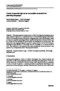
We will now describe the prototype we have constructed, called ASPA , for computing answer sets of programs with aggregates. The computation is performed following the semantics given in Definition 14, simplified by Theorem 2. In other words, to compute the answer set of a program P , we 1. Compute a complete (and possibly minimal) solution set for each aggregate atom occurring in P ; 2. Unfold P using the computed solution sets; 3. Compute the answer sets of the unfolded program unf olding(P ) using a standard answer set solver (in our case, both Smodels and Cmodels). The overall structure of the system is shown in Figure 2. ASP A Program
ground program with aggregates
Preprocessor
Lparse pipe
unfolded ground normal logic program
Transformer pipe
simplified ground normal logic program
Lparse pipe
pipe
Answer Sets
ASP Solver (Smodels, Cmodels, ...)
Figure 2: Overall System Structure
The computation of answer sets is performed in five steps. In the first step, a preprocessor performs a number of simple syntactic transformations on the input program, which are aimed at rewriting the aggregate atoms in a format acceptable by lparse. For example, the aggregate atom Sum({X | p(X)}) ≥ 40 is rewritten to “$agg”(sum, “$x”, p(“$x”), 40, geq) and an additional rule 0 {‘‘$agg’’(sum,‘‘$x’’, p(‘‘$x’’), 40, geq)} 1 is added to the program. The rewritten program is then grounded and simplified using lparse, in which aggregate atoms are treated like standard (non-aggregate) literals. The ground program is processed by the transformer module, detailed in Figure 3, in which the unfolded program is computed. This module performs the following operations: 1. Creation of the atom table, the aggregate table, and the rule table, used to store the ground atoms, aggregate atoms, and rules of the program, respectively. This is performed by the Reader component in Figure 3. 2. Identification of the dependencies between aggregate atoms and the atoms contributing to such atoms (done by the Dependencies Analyzer);
16
GROUND ASP PROGRAM
A
READER
ATOMS TABLE
AGGREGATES TABLE
AGGREGATES DEPENDENCIES
COMPLETE SOLUTION SET
AGGREGATE CONSTRAINT
DEPENDENCIES ANALYZER
RULES TABLE
AGGREGATE SOLVER
RULES EXPANDER
GROUND ASP PROGRAM
Figure 3: Transformer Module 3. Computation of a complete solution set for each aggregate atom (done by the Aggregate Solver—as described in the previous subsection); 4. Creation of the unfolded program (done by the Rule Expander). Note that the unfolded program is passed one more time through lparse, to avail of the simplifications and optimizations that lparse can perform on a normal logic program (e.g., expansion of domain predicates and removal of unnecessary rules). The resulting program is a ground normal logic program, whose answer sets can be computed by a system like Smodels or Cmodels. 3.4.3
Some Experimental Results
We have performed a number of tests using the ASPA system. In particular, we selected benchmarks with aggregates presented in the literature. The benchmarks, drawn from various papers on aggregation, are: • Company Control: Let owns(X, Y, N ) denotes the fact that company X owns a fraction N of the shares of the company Y . We say that a company X controls a company Y if the sum of the shares it owns in Y together with the sum of the shares owned in Y by companies
17
controlled by X is greater than half of the total shares of Y : control shares(X, Y, N ) ← owns(X, Y, N ) control shares(X, Y, N ) ← control(X, Z), owns(Z, Y, N ) control(X, Y ) ← Sum({{ M | control shares(X, Y, M ) }}) > 50 We explored different instances, with varying numbers of companies. • Shortest Path: Suppose a weight-graph is given by relation arc, where arc(X, Y, W ) means that there is an arc in the graph from node X to node Y of weight W . We represent the shortest path (minimal weight) relation spath using the following rules path(X, Y, C) ← arc(X, Y, C) path(X, Y, C) ← spath(X, Z, C1), arc(Z, Y, C2), C = C1 + C2 spath(X, Y, C) ← Min({{ D | path(X, Y, D) }}) = C The instances explored make use of graphs with varying number of nodes. • Party Invitations: The main idea of this problem is to send out party invitations considering that some people will not accept the invitation unless they know that at least k other people from their friends accept it too. f riend(X, Y ) coming(X) coming(X) come f riend(X, Y )
← ← ← ←
f riend(Y, X) requires(X, 0) requires(X, K), Count({ Y | come f riend(X, Y ) }) ≥ K f riend(X, Y ), coming(Y )
The instances explored in our experiments have different numbers of people invited to the party. • Group Seating: In this problem, we want to arrange the sitting of a group of n people in a restaurant, knowing that the number of tables times the number of seats on each table equals to n. The number of people that can sit at a table cannot exceed the number of chairs at this table, and each person can sit exactly at one table. In addition, people who like each other must sit together at the same table and those who dislike each other must sit at different tables. at(P, T ) ← person(P ), table(T ), not not at(P, T ) not at(P, T ) ← person(P ), table(T ), not at(P, T ) ← table(T ), nchairs(C), Count({ P | at(P, T ) }) > C ← person(P ), Count({ T | at(P, T ) }) 6= 1 ← like(P 1, P 2), at(P 1, T ), not at(P 2, T ) ← dislike(P 1, P 2), at(P 1, T ), at(P 2, T ) The benchmark makes use of 16 guests, 4 tables, each having 4 chairs. • Employee Raise: Assume that a manager decides to select at most N employees to give them a raise. An employee is a good candidate for the raise if he has worked for at least K hours
18
per week. A relation emp(X, D, H) denotes that an employee X worked H hours during the day D. raised(X) ← empN ame(X), not notraised(X) notraised(X) ← empN ame(X), not raised(X) notraised(X) ← empN ame(X), nHours(K), Sum({{H | emp(X, D, H) }}) < K ← maxRaised(N ), Count({X | raised(X)}) > N The different experiments conducted are described by the two parameters M/N , where M is the number of employees and N the maximum number of individuals getting a raise. • NM1 and NM2 : these are two synthetic benchmarks that compute large aggregates that are recursive and non-monotonic. NM1 has its core in the following rules: q(K) p(X) a(X) b(X)
← ← ← ←
r(X), w(K), max(X | p(X)) = K q(K), r(X), w(K) notb(X), p(X), r(X) nota(X), p(X), r(X)
The program NM2 relies on the following set of rules: q(K) ← r(X), w(K), min(X | p(X)) > K p(X) ← q(K), r(X), w(K) The code for the benchmarks can be found at: www.cs.nmsu.edu/~ielkaban/asp-aggr.html. Table 1 presents the results obtained. The columns of the table have the following meaning: • Program is the name of the benchmark. • Instance describes the specific instance of the benchmark used in the test. • Smodels Time is the time (in seconds) employed by Smodels to compute the answer sets of the unfolded program. • Cmodels Time is the time (in seconds) employed by Cmodels to compute the answer sets of the unfolded program. • Transformer Time is the time (in seconds) to preprocess and ground the program (i.e., compute the solutions of aggregates and perform the unfolding—this includes the complete pipeline discussed in Figure 2). • DLVA is the time employed by the DLVA system to execute the same benchmark (where applicable, otherwise marked N/A)—observe that the current distribution of this system does not support recursion through aggregates. All computations have been performed on a Pentium 4, 3.06 GHz machine with 512MB of memory under Linux 2.4.28 using GCC 3.2.1. The system is available for download at www.cs.nmsu.edu/ ~ielkaban/asp-aggr.html. As we can see from the table, even this relatively simple implementation of aggregates can efficiently solve all benchmarks we tried, offering a coverage significantly larger than other existing implementations. Observe also that the overhead introduced by the computation of aggregate solutions is significant in very few cases. 19
Program
Instance
Smodels Time
Cmodels Time
Transformer Time
DLVA Time
(Preprocessor, Lparse, Transformer, and Lparse) Company Control Company Control Company Control Company Control Shortest Path Shortest Path Shortest Path Shortest Path (All Pairs) Party Invitations Party Invitations Party Invitations Seating Seating Employee Raise Employee Raise Employee Raise NM1 NM1 NM2 NM2
20 40 80 120 20 30 50 20 40 80 160 9/3/3 16/4/4 15/5 21/15 25/20 125 150 125 150
0.010 0.020 0.030 0.040 0.220 0.790 3.510 6.020 0.010 0.020 0.050 0.04 11.40 0.57 2.88 3.42 1.10 1.60 1.44 2.08
0.00 0.00 0.00 0.030 0.05 0.13 0.51 1.15 0.00 0.01 0.02 0.03 3.72 0.87 1.75 8.38 0.07 0.18 0.23 0.34
0.080 0.340 2.850 12.100 0.740 2.640 13.400 35.400 0.010 0.030 0.050 0.01 0.330 0.140 1.770 5.20 1.00 1.30 0.80 1.28
N/A N/A N/A N/A N/A N/A N/A N/A N/A N/A N/A 0.03 4.337 2.750 6.235 3.95 N/A N/A N/A N/A
Table 1: Computing Answer Sets of Benchmarks with Aggregates
4
An Alternative Semantical Characterization
The main advantage of the previously introduced definition of ASPA -answer sets is its simplicity, which allows an easy computation of answer sets of programs with aggregates using currently available answer set solvers. Following this approach, all we need to do to compute answer sets of a program P is to compute its unfolded program unf olding(P ) and then use an answer set solver to compute the answer sets of unf olding(P ). One disadvantage of this method lies in the fact that the size of the program unf olding(P ) can be exponential in the size of P —which could potentially become unmanageable. Theoretically, this is not a surprise, as the problem of determining the existence of answer sets for propositional programs with aggregates can be very complex, depending on the types of aggregates (i.e., aggregate functions and comparison predicates) present in the program (see [39] and Chapter 6 in [32] for a thorough discussion of these issues). In what follows, we present an alternative characterization of the semantics for programs with aggregates, whose underlying principle is still the unfolding mechanism. This new characterization allows us to compute the answer sets of a program by using a generate-and-test procedure. The key difference is that the unfolding is now performed with respect to a given interpretation.
4.1
Unfolding with respect to an Interpretation
Let us start by specializing the notion of solution of an aggregate to the case of a fixed interpretation. Definition 17 (M -solution) For a ground aggregate atom ℓ and an interpretation M , its M -
20
solution set is SOLN ∗ (ℓ, M ) = {Sℓ | Sℓ ∈ SOLN (ℓ), Sℓ .p ⊆ M, Sℓ .n ∩ M = ∅} . Intuitively, SOLN ∗ (ℓ, M ) is the set of solutions of ℓ which are V true in M . For a solution Sℓ ∈ SOLN ∗ (ℓ, M ), the unfolding of ℓ w.r.t. Sℓ is the conjunction a∈Sℓ .p a. We say that ℓ′ is an unfolding of ℓ with respect to M if ℓ′ is an unfolding of ℓ with respect to some Sℓ ∈ SOLN ∗ (ℓ, M ). When SOLN ∗ (ℓ, M ) = ∅, we say that ⊥ is the only unfolding of ℓ in M . We next define the unfolding of a program with respect to an interpretation M . Definition 18 (Unfolding w.r.t. an Interpretation) Let M be an interpretation of the program P . The unfolding of a rule r ∈ ground(P ) w.r.t. M is a set of rules, denoted by unf olding∗ (r, M ), defined as follows: 1. If neg(r) ∩ M 6= ∅, or if there is a c ∈ agg(r) such that ⊥ is the unfolding of c in M , then unf olding∗ (r, M ) = ∅; 2. If neg(r) ∩ M = ∅ and, for every c ∈ agg(r) ⊥ is not the unfolding of c, then r ′ ∈ unf olding∗ (r, M ) if (a) head(r ′ ) = head(r) (b) there exists a sequence of aggregate solutions hSc ic∈agg(r) of aggregate atoms S in agg(r) ∗ ′ such that Sc ∈ SOLN (c, M ) for every c ∈ agg(r) and pos(r ) = pos(r) ∪ c∈agg(r) Sc .p.
The unfolding of P w.r.t. M , denoted by unf olding∗ (P, M ), is defined as follows: [ unf olding∗ (P, M ) = unf olding∗ (r, M ) r∈ground(P )
Observe that unf olding∗ (P, M ) is a definite program. Similar to the definition of an answer set in [14], we define answer sets as follows. Definition 19 M is an ASPA -answer set of P iff M is an answer set of unf olding∗ (P, M ). In the next example, we illustrate the above definitions. Example 7 Consider the program P1 (Example 3) and consider the interpretation M {p(a), p(b)}. Let ℓ be the aggregate atom Count({X | p(X)}) > 0. We have that
=
SOLN ∗ (ℓ, M ) = {h{p(a)}, ∅i, h{p(b)}, ∅i, h{p(a), p(b)}, ∅i} The unf olding∗ (P1 , M ) is: p(a) ← p(a) p(a) ← p(a), p(b)
p(a) ← p(b) p(b) ←
Observe that M is indeed an answer set of unf olding∗ (P1 , M ).
21
2
Example 8 Consider the program P2 from Example 4, and let us consider M = {p(1), p(2), p(3), p(5), q}. Observe that, if we consider the aggregate atom ℓ of the form Sum({X | p(X)}) > 10 then SOLN ∗ (ℓ, M ) = {h{p(1), p(2), p(3), p(5)}, ∅i} Then, unf olding∗ (P2 , M ) is: p(1) ← p(3) ← q ← p(1), p(2), p(3), p(5)
p(2) ← p(5) ← q
This program has the unique answer set {p(1), p(2), p(3)} which is different from M ; thus M is not an answer set of P2 according to Definition 19. 2 The next theorem proves that this new definition is equivalent to the one in Section 3. Theorem 3 For any ASPA program P , an interpretation M of P is an answer set of unf olding(P ) iff M is an answer set of unf olding∗ (P, M ). Proof. Let R = unf olding∗ (P, M ) and Q = (unf olding(P ))M . We have that R and Q are definite programs. We will prove by induction on k that if M is an answer set of Q then TQ ↑ k = TR ↑ k for every k ≥ 0.7 The equation holds trivially for k = 0. Let us consider the case for k > 0, assuming that TQ ↑ l = TR ↑ l for 0 ≤ l < k. • Consider p ∈ TQ ↑ k. This means that there exists some rule r ′ ∈ Q such that head(r ′ ) = p and body(r ′ ) ⊆ TQ ↑ k − 1. From the definition of the Gelfond-Lifschitz reduction and the definition of the unfolded program, we can conclude that there exists some rule r ∈ ground(P ) and a sequence of aggregate solutions hSc ic∈agg(r) S for the aggregate atoms in body(r) such that S pos(r ′ ) = pos(r) ∪ c∈agg(r) Sc .p, and (neg(r) ∪ c∈agg(r) Sc .n) ∩ M = ∅. In other words, r ′ is the Gelfond-Lifschitz reduction with respect to M of the unfolding of r with respect to hSc ic∈agg(r) . These conditions imply that r ′ ∈ R. Together with the inductive hypothesis, we can conclude that p ∈ TR ↑ k. • Consider p ∈ TR ↑ k. Thus, there exists some rule r ′ ∈ R such that head(r ′ ) = p and body(r ′ ) ⊆ TR ↑ k − 1. From the definition of R, we can conclude that there exists some rule r ∈ ground(P ) and a sequence of aggregate solutions hSc ic∈agg(r) for S the aggregate atoms in S ′ body(r) such that pos(r ) = pos(r) ∪ c∈agg(r) Sc .p, and (neg(r) ∪ c∈agg(r) Sc .n) ∩ M = ∅. Thus, r ′ ∈ Q. Together with the inductive hypothesis, we can conclude that p ∈ TQ ↑ k. This shows that, if M is an answer set of Q, then M is an answer set of R. Similar arguments can be used to show that if M is an answer set of R, TQ ↑ k = TR ↑ k for every k ≥ 0, which means that M is an answer set of Q. 2 The above theorem shows that we can compute answer sets of aggregate programs in the same generate–and–test order as in normal logic programs. Given a program P and an interpretation M , instead of computing the Gelfond-Lifschitz’s reduct P M we compute the unf olding∗ (P, M ). This method of computation might yield better performance but requires modifications of the answer set solver. Another advantage of this alternative characterization is its suitability to handle aggregate atoms as heads of program rules, as discussed next. 7
TR denotes the traditional immediate consequence operator and TR ↑ k is the kth upward iteration of TR .
22
4.2
Aggregates in the Head of Rules
As in most earlier proposals, with the exception of the weight constraints of Smodels [30], logic programs with abstract constraint atoms [26], and answer sets for propositional theories [13], the language discussed in Section 2 does not allow aggregate atoms as facts (or as head of a rule). To motivate the need for aggregate atoms as rule heads, let us consider the following example. Example 9 Let us have a set of three students who have taken an exam, and let us assume that at least two got ’A’. This can be encoded as the Smodels program with the set of facts about students and the weight constraint 2{gotA(X) : student(X)} If aggregate atoms were allowed in the head, we could encode this problem as the following ASPA program Count({X | gotA(X)}) ≥ 2 along with a constraint stating that if gotA(X) is true then student(X) must be true as well—which can be encoded using the constraint ⊥ ← gotA(X), not student(X) This program should have four answer sets, each representing a possible grade distribution, in which either one of the students does not receive the ’A’ grade or all the three students receive ’A’. 2 The above example suggests that aggregate atoms in the head of a rule are convenient for certain knowledge representation tasks. We will now consider logic programs with aggregate atoms in which each rule is an expression of the form D ← C1 , . . . , Cm , A1 , . . . , An , not B1 , . . . , not Bk
(2)
where A1 , . . . , An , B1 , . . . , Bk are ASP-atoms, C1 , . . . , Cm are aggregate atoms (m ≥ 0, n ≥ 0, k ≥ 0), and D can be either an ASP-atom or an aggregate atom. An ASPA program is now a collection of rules of the above form. The notion of a model can be straightforwardly generalized to program with aggregates in the head. It is omitted here for brevity. As it turns out, the semantics presented in the previous subsection can be easily extended to allow for aggregate atoms in the head of rules. It only requires an additional step, in order to convert programs with aggregates in the head to programs without aggregates in the head. To achieve that, we introduce the following notation. Definition 20 Let P be a program with aggregates in the head, M be an interpretation of P , and r be one of the rules in ground(P ) such that head(r) is an aggregate atom. We define r ⊥ = {⊥ ← body(r)} and r M = {p ← body(r) | p ∈ H(head(r)) ∩ M }. Definition 21 Let P be a program with aggregates in the head and let M be an interpretation of P . The aggregate-free head reduct of P with respect to M , denoted by P (M ), is the program obtained from P by replacing each rule r ∈ ground(P ) whose head is an aggregate atom with (a) r ⊥ if SOLN ∗ (head(r), M ) = ∅; or (b) r M if SOLN ∗ (head(r), M ) 6= ∅. 23
For each rule r, whose head is an aggregate atom, we first check whether head(r) is satisfied by M (i.e., SOLN ∗ (head(r), M ) = ∅ by Observation 3.1). If it is not satisfied, then this means that we intend the rule’s body to not be satisfied—and we encode this with a rule of the type r ⊥ . Otherwise, M provides us with a solution of the aggregate atom head(r)—i.e., hM ∩ H(head(r)), H(head(r)) \ M i—and we intend to use this rule to “support” such solution; in particular, the rules in r M provides support for all the elements in M ∩ H(head(r)). We are now ready to define the notion of answer sets for program with aggregates in the head. Definition 22 A set of atoms M is an ASPA -answer set of P iff M is an answer set of unf olding∗ (P (M ), M ). Observe that, because of aggregates in the head, an ASPA -answer set might be non minimal. Nevertheless, the following holds. Observation 4.1 Every ASPA -answer set of a program P is a model of P . Example 10 Consider the program P5 : student(a) student(b) student(c) Count({X | gotA(X)}) ≥ 2 ⊥ Let us compute some answer sets of P5 . gotA(X)}) ≥ 2.
← ← ← ← ← gotA(X), not student(X) Let ℓ denote the aggregate atom Count({X |
• Let M1 = {student(a), student(b), student(c), gotA(a)}. We can check that ℓ is not satisfied by M1 , and hence, the unfolding of the fourth rule of P5 is the set of rules {⊥}, i.e., unf olding∗ (P5 (M1 ), M1 ) is the following program: student(a) student(b) student(c) ⊥ ⊥
← ← ← ← gotA(X), not student(X)
This program does not have any answer set. Thus, M1 is not an ASPA -answer set of P5 (according to Definition 22). • Consider M2 = {student(a), student(b), student(c), gotA(a), gotA(b)}. We have that ℓ is satisfied by M2 . Hence, unf olding∗ (P5 (M2 ), M2 ) is obtained from P5 by replacing its fourth rule with the two rules gotA(a) ← gotA(b) ← unf olding∗ (P5 (M2 ), M2 ) has M2 as an answer set. Therefore, M2 is an ASPA -answer set of P5 . 24
Similar to the second item, we can show that M3 = {student(a), student(b), student(c), gotA(a), gotA(c)} M4 = {student(a), student(b), student(c), gotA(b), gotA(c)} M5 = {student(a), student(b), student(c), gotA(a), gotA(b), gotA(c)} are answer sets of P5 .
5
2
Related Work
In this section, we relate our definition of ASPA -answer sets to several formulations of aggregates proposed in the literature. We begin with a comparison of our unfolding approach with the two most recently proposed semantics for LP with aggregates, i.e., the ultimate stable model semantics [32–34], the minimal answer set semantics [12, 13], and the semantics for abstract constraint atoms [26]. We then relate our work to earlier proposals, such as perfect models of aggregate-stratified programs (e.g., [28]), the fixpoint answer set semantics of aggregate-monotonic programs [20], and the semantics of programs with weight constraints [30]. Finally, we briefly discuss the relation of ASPA -answer sets to other proposals.
5.1
Pelov’s Approximation Semantics for Logic Program with Aggregates
The doctoral thesis of Pelov [32] contains a nice generalization of several semantics of logic programs to the case of logic programs with aggregates. The key idea in his work is the use of approximation theory in defining several semantics for logic programs with aggregates (e.g., two-valued semantics, ultimate three-valued stable semantics, three-valued stable model semantics). In particular, in [32], the author describes a fixpoint operator, called Φappr , operating on 3-valued interpretations and P parameterized by the choice of approximating aggregates. The results presented in [39] allow us to conclude the following result. Proposition 1 Given a program with aggregates P , M is a ASPA answer set of P if and only if . denotes the first component of Φaggr (·, M ), where Φaggr,1 M is the least fixpoint of Φaggr,1 P P P The work of Pelov includes also a translation of logic programs with aggregates to normal logic programs, denoted by tr, which was first given in [33] and then in [32]. The translation in [33] (independently developed) and the unfolding proposed in Section 2 have strong similarities8 . For the completeness of the paper, we will review the basics of the translation of [33], expressed using our notation. Given a logic program with aggregates P , tr(P ) denotes the normal logic program obtained after the translation. The translation begins with the translation of each aggregate atom W H(s) ℓ = P(s) into a disjunction tr(ℓ) = F(s1 ,s2 ) where H(s) is the set of atoms of p—the predicate of H(s)
s—in BP , (s1 , s2 ) belongs to an index set, s1 ⊆ s2 ⊆ H(s), and each F(s1 ,s2) is a conjunction of the form ^ ^ not l l∧ l∈s1
l∈s\s2
8
We would like to thank a reviewer of an earlier version of this paper who provided us with the pointers to these works.
25
The construction of tr(ℓ) considers only pairs (s1 , s2 ) satisfying the following condition: every interpretation I such that s1 ⊆ I and s\s2 ∩I = ∅ also satisfies ℓ. tr(P ) is then created by rewriting rules with disjunction in the body by a set of rules in a straightforward way. For example, the rule a ← (b ∨ c), d is replaced by the two rules a ← b, d a ← c, d We can prove a lemma that connects unf olding(P ) and tr(P ). H(s)
Lemma 3 For every aggregate atom ℓ = P(s), S is a solution of ℓ if and only if F(S.p,S.p∪(H(s)\S.n)) is a disjunct in tr(ℓ). Proof. The result is a trivial consequence of the definition of a solution and the definition of tr(ℓ). 2 This lemma allows us to prove the following relationship between unf olding(P ) and tr(P ). Corollary 5.1 For every program P , A is an ASPA -answer set of P if and only if A is an exact stable model of P with respect to [34]. Proof. The result is a trivial consequence of the fact that unf olding(P ) = tr(P ) and tr(P ) has the same set of partial stable models as P [33]. 2
5.2
ASPA -Answer Sets and Minimality Condition
In this subsection, we investigate the relationship between ASPA -answer sets and the notion of answer set defined by Faber et al. in [12]. The notion of answer set proposed in [12] is based on a new notion of reduct, defined as follows. Given a program P and a set of atoms S, the reduct of P with respect to S, denoted by S P , is obtained by removing from ground(P ) those rules whose body is not satisfied by S. In other words, S
P = {r | r ∈ ground(P ), S |= body(r)}.
The novelty of this reduct is that it does not remove aggregate atoms and negation-as-failure literals satisfied by S. Definition 23 (FLP-answer set, [12]) For a program P , S is a FLP-answer set of P iff it is a minimal model of S P . Observe that the definition of an answer set in this approach explicitly requires answer sets to be minimal, thus requiring the ability to determine minimal models of a program with aggregates. In the following propositions, we will show that ASPA -answer sets of a program P are FLP-answer sets and that FLP-answer sets of P are minimal models of unf olding(P ), but not necessary ASPA answer sets. Theorem 4 Let P be a program with aggregates. If M is an ASPA -answer set, then M is a FLPanswer set of P . If M is a FLP-answer set of P then M is a minimal model of unf olding(P ). 26
Proof. • Let Q = unf olding(P ). Since M is an ASPA -answer set, we have that M is an answer set of Q. Lemma 2 shows that M is a model of ground(P ) and hence is a model of R = M (ground(P )). Let us assume that M is not a minimal model of R. This means that there exists M ′ ( M such that M ′ is a model of M (P ). We will show that M ′ is a model of Q′ = QM where QM is the result of the Gelfond-Lifschitz transformation of the program Q with respect to M . Consider a rule r2 ∈ Q′ such that M ′ |= body(r2 ), i.e., pos(r2 ) ⊆ M ′ . From the definition of the Gelfond-Lifschitz transformation, we conclude that there exists some r ′ ∈ Q such that pos(r ′ ) = pos(r2 ) and neg(r ′ ) ∩ M = ∅. This implies that there is a rule r ∈ ground(P ) and a sequence of solutions hSc ic∈agg(r) of aggregates in r such that r ′ is the unfolding of r with respect to hSc ic∈agg(r) and for every c ∈ agg(r), Sc .p ⊆ M ′ and Sc .n ∩ M = ∅. Since M ′ ⊆ M , we can conclude that M |= body(r), i.e., r ∈ R. Furthermore, M ′ |= body(r) because pos(r) ⊆ pos(r ′ ) = pos(r2 ) ⊆ M ′ , neg(r) ⊆ neg(r ′ ) and neg(r ′ ) ∩ M = ∅, and for every c ∈ agg(r), Sc .p ⊆ M ′ and Sc .n ∩ M ′ = ∅. Since M ′ is a model of R, we have that head(r) ∈ M ′ . Since head(r2 ) = head(r ′ ) = head(r), we have that M ′ satisfies r2 . This holds for every rule of Q′ . Thus, M ′ is a model of Q. This contradicts the fact that M is an answer set of Q. • Let M be a FLP-answer set of P . Clearly, M is a model of ground(P ) and hence of unf olding(P ). If M is not a minimal model of unf olding(P ), there exists some M ′ ( M which is a model of unf olding(P ). Lemma 1 implies that M ′ is a model of ground(P ) and hence is a model of M P . This is a contradiction with the assumption that M is a FLP-answer set of P . Thus, we can conclude that M is a minimal model of unf olding(P ). 2 The next example shows that FLP-answer sets might not be ASPA -answer sets.9 Example 11 Consider the program P6 where p(1) ← Sum({X | p(X)}) ≥ 0 p(1) ← p(−1) p(−1) ← p(1) The interpretation M = {p(1), p(−1)} is a FLP-answer set of P6 . We will show next that P6 does not have an answer set according to our definition. It is possible to show10 that the aggregate atom Sum({X | p(X)}) ≥ 0 has the following solutions with respect to BP = {p(1), p(−1)}: h∅, {p(−1)}i, h∅, {p(1), p(−1)}i, h{p(1)}, {p(−1)}i, h{p(1)}, ∅i, and h{p(1), p(−1)}, ∅i. The unfold9 10
We would like to thank an anonymous reviewer of an earlier version of this paper who suggested this example. We follow the common practice that the sum of an empty set is equal to 0.
27
ing of P6 , unf olding(P6 ), consists of the following rules: p(1) p(1) p(1) p(1) p(1) p(1) p(−1)
← ← ← ← ← ← ←
not p(−1) not p(1), not p(−1) p(1), not p(−1) p(1) p(1), p(−1) p(−1) p(1)
It is easy to see that unf olding(P6 ) does not have answer sets. Thus, P6 does not have ASPA -answer sets. 2 Remark 2 If we replace in P6 the rule p(1) ← Sum({X | p(X)}) ≥ 0 with the intuitively equivalent Smodels weight constraint rule p(1) ← 0[p(1) = 1, p(−1) = −1]. we obtain a program that does not have answer sets in Smodels. The above example shows that our characterization of programs with aggregates differs from the proposal in [12]. Apart from the lack of support for aggregates in the heads of rules, the semantics of [12] might accept answer sets that are not ASPA -answer sets. Observe that the two semantical characterizations coincide for large classes of programs (e.g., for programs that have only monotone aggregates).
5.3
Logic Programs with Abstract Constraint Atoms
A very general semantic characterization of programs with aggregates has been proposed by Marek and Truszczy´ nski in [26]. The framework offers a model where general aggregates can be employed both in the body and in the head of rules. The authors introduce the notion of abstract constraint atom, (X, C), where X is a set of atoms (the domain of the aggregate) and C is a subset of 2X (the solutions of the aggregate). For an abstract constraint atom A = (X, C), we will denote X with AD and C with AC . In [26], the focus is only on monotone constraints, i.e., constraints (X, C), where if Y ∈ C then all supersets of Y are also in C. A program with monotone constraints is a set of rules of the form B0 ← B1 , . . . , Bn , not Bn+1 , . . . , not Bn+m where each Bi (i ≥ 0) is an abstract constraint atom. Abusing the notation, for a rule r of the above form, we use head(r), pos(r), neg(r), and body(r) to denote B0 , {B1 , . . . , Bn }, {Bn+1 , . . . , Bn+m }, and {B1 , . . . , Bn , notBn+1 , . . . , notBn+m}, respectively. The semantics of this language is developed as a generalization of answer set semantics for normal logic programs. To make the paper selfcontained, we briefly review the notion of a stable model for a program with monotone constraints. An interpretation M satisfies A = (X, C), denoted by M |= A, if X ∩M ∈ C (or AD ∩M ∈ AC ). M |= not A if M 6|= A. For a set of literals S, M |= S if M |= B for each B ∈ S. For a program with monotone constraints P , hset(P ) denotes the set ∪r∈P head(r)d . Given a set of atoms S, a rule r is applicable in S if S |= body(r). The set of applicable rules in S is denoted by P (S). A set S ′ is 28
nondeterministically one-step provable from S by means of P if S ′ ⊆ hset(P (S)) and S ′ |= head(r) for every r ∈ P (S). The nondeterministic one-step provability operator TPnd is a function from 2A A to 22 , where A denotes the Herbrand base of P , such that for every S ⊆ A, TPnd (S) consists of all sets S ′ that are nondeterministically one-step provable from S by means of P . A sequence t = (Xn )n=0,1,2,... is called a P-computation if X0 = ∅ and for every non-negative integer n, (i) Xn ⊆ Xn+1 , and (ii) Xn+1 ∈ TPnd (Xn ). St = ∪ ∞ n=0 Xi is called the result of the computation t. A set of atoms S is a derivable model of P if there exists a P -computation t such that S = St . For a monotone program P and a set of atoms M , the reduct of P with respect to M , denoted by P M , is obtained from P by (i) removing from P every rule containing in the body a literal not A such that M |= A; and (ii) removing all literals of the form not A from the remaining rules. A set of atoms M is an stable model of a monotone program P if M is a derivable model of the reduct P M . Observe that each aggregate atom ℓ in our notation can be represented by an abstract constraint atom (H(ℓ), Cℓ ), where Cℓ = {S | S ⊆ H(ℓ), S |= ℓ}. Furthermore, an atom a can be represented as an abstract constraint atom ({a}, {{a}}). Thus, each program P , as a set of rules of the form (2), could be viewed as a program with abstract constraint atoms PA , where PA is obtained from P by replacing every occurrence of an aggregate atom ℓ or an atom a in P with (H(ℓ), Cℓ ) or ({a}, {{a}}) respectively. The monotonicity of an abstract constraint atom implies the following: Observation 5.1 Let ℓ be an aggregate atom and M be a set of atoms such that Cℓ (H(ℓ)) is a monotone constraint and M |= Cℓ (H(ℓ)). Then, hM ∩ H(ℓ), ∅i is a solution of ℓ. Using this observation, we can related the notions of ASPA -answer set and of stable models for programs with monotone atoms as follows. Theorem 5 Let P be a program with monotone aggregates. M is an ASPA answer set of P iff M is a stable model of PA according to [26]. Proof. For each rule r ∈ P , let rA be the rule in PA which is obtained from r by the translation from P to PA . “⇐=” Let usS assume M is a stable model of PA according to [26]. A result in [26] shows that M= ∞ 0 Xi where X0 = ∅ Xi+1 = M ∩ hset(P (Xi )) We will show that M is a ASPA answer set of P by proving that lf p(TQ ) = M where Q = unf olding∗ (P ′ , M ) and P ′ the aggregate-free head reduct of P with respect to M (Definition 21). Let us start by showing that Xi ⊆ TQ ↑ i for i ≥ 0, using induction on i. The result is obvious for i = 0. Let us assume the result to hold for i ≤ k and let us consider the case of Xk+1 . By the definition of Xi ’s, p ∈ Xk+1 implies that p ∈ M ∩ hset(PA (Xk )). This means that there is a rule A ← B1 , . . . , Bn ∈ PAM (3) 29
such that Xk |= Bi for i = 1, . . . , n, AD ∩M ∈ AC , and p ∈ AD ∩M . From Xk ∩(Bi )D ∈ (Bi )C , Xk ∩(Bi )D ⊆ TQ ↑ k∩(Bi )D , and the monotonicity of Bi , we have that TQ ↑ k∩(Bi )D ∈ (Bi )C . From Observation 5.1 and the monotonicity of the aggregates, we can infer that there is a rule in Q with head(r) = p and TQ ↑ k |= body(r). Thus, p ∈ TQ ↑ (k + 1). The inductive step is proved. This allows us to conclude that M ⊆ lf p(TQ ). On the other hand, we can easily show that M is a model of Q, thus lf p(TQ ) ⊆ M . This allows us to conclude that M = lf p(TQ ). Together with M ⊆ lf p(TQ ), we have that M is an ASPA answer set of P . “=⇒” Let M be an ASPA answer set of P and Q = unf olding∗ (P ′ , M ) where P ′ is the aggregate-free head reduct of P with respect to M . Thus, M = lf p(TQ ). We will prove that M is a stable model of P by showing that the sequence Xi = TQ ↑ i, for i ≥ 0, is a P-computation. Obviously, we have that (i.) X0 = ∅ and (ii) Xi ⊆ Xi+1 for i ≥ 0. It remains to be shown that (iii) Xi+1 ∈ TPnd (Xi ) for i ≥ 0. In order to prove the property (iii) we need to show that (iv) Xi+1 ⊆ hset(PA (Xi )) and (v) Xi+1 |= head(r) for each rA in PA (Xi ). Let us consider p ∈ Xi+1 = TQ ↑ i + 1. This means that there exists some rule r ′ in Q such that body(r ′ ) ⊆ Xi and head(r ′ ) = p. Let r be the rule in P such that r ′ is obtained from r (as specified in Definitions 21-18). This implies neg(r) ∩ M = ∅, pos(r) ⊆ Xi , and Xi |= c for every c ∈ agg(r). From the monotonicity of aggregates in P , we can conclude that rA ∈ PA (Xi ) and p ∈ head(rA )D . This holds for every p ∈ Xi+1 . Hence, we have that Xi+1 ⊆ hset(PA (Xi )), i.e., (iv) is proved. Now let us consider a rule rA ∈ PA (Xi ). This implies that the rule r, from which rA is obtained, satisfies that neg(r) ∩ M = ∅, pos(r) ⊆ Xi , and Xi |= c for every c ∈ agg(r). Again, the monotonicity of aggregates in P implies that M |= c for every c ∈ agg(r). By the definition of Q, we have that for each p ∈ head(rA )D ∩ M , there exists a rule rp ∈ Q such that p = head(rp ) and body(rp ) ⊆ Xi . As such, head(rA )D ∩ M ⊆ Xi+1 . This means that Xi+1 |= head(rA ), i.e., (v) is proved. 2
5.4
Answer Sets for Propositional Theories
The proposal of Ferraris [13] applies a novel notion of reduct and answer sets, developed for propositional theories, to the case of aggregates containing arbitrary formulae. The intuition behind the notion of satisfaction of an aggregate relies on translating aggregates to propositional formulae that guarantee that all cases where the aggregate is false are ruled out. In particular, for an aggregate of the form F ({α1 = w1 , . . . , αk = wk }) ⊙ R, where αi are propositional formulae, wj and R are real numbers, F is a function from multisets of real numbers to R ∪ {+∞, −∞}, and ⊙ is a relational operator (e.g., ≤, 6=), the transformation leads to the propositional formula: ! _ ^ ^ αi αi ⇒ I ⊆ {1, . . . , k} F ({wi | i ∈ I}) 6 ⊙R
i∈I
30
i∈{1,...,k}\I
The results in [13] show that the new notion of reduct, along with this translation for aggregates, applied to the class of logic programs with aggregates of [12], captures exactly the class of FLPanswer sets.
5.5
Logic Programs with Weight Constraints
Let us consider the weight constraints employed by Smodels and let us describe a translation method to convert them into our language with aggregates. We will focus on weight constraint that are used in the body of rules (see Sect. 4.2 for aggregates in the heads of rules). For simplicity, we will also focus on weight constraints with non-negative weights (the generalization can be obtained through algebraic manipulations, as described in [30]). A ground weight constraint c has the form:11 L ≤ {p1 =w1 , . . . , pn =wn , not r1 =v1 , . . . , not rm =vm } ≤ U where pi , rj are ground atoms, and wi , vj , L, U are numeric constants. pi ’s and not rj ’s are called literals of c. lit(c) denotes the set of literals of c. The local weight function of a constraint c, w(c), returns the weight of its literals. For example, w(c)(pi ) = wi and w(c)(not ri ) = vi . The weight of a weight constraint c in a model S, denoted by W (c, S), is given by X X w(c)(p) + w(c)(not p). W (c, S) = p∈lit(c), p∈S
not q∈lit(c), q ∈S /
We will now show how weight constraints in Smodels can be translated into aggregates in our language. For each weight constraint c, let aggc+ and aggc− be two new predicates which do not belong to the language of P . Let r(c) be the set of following rules: aggc+ (1, w1 ) ← p1 . aggc− (1, v1 ) ← r1 .
··· ···
aggc+ (n, wn ) ← pn . aggc− (m, vm ) ← rm .
Intuitively, aggc+ , aggc− assign a specific weight to each literal originally present in the weight constraint. The weight constraint itself is replaced by a conjunction τ (c): � Sum({{X | ∃Y.aggc+ (Y, X)}}) = S +P∧ Sum({{X | ∃Y.aggc− (Y, X)}}) = S − ∧ τ (c) = − L ≤ S+ + m i=1 vi − S ≤ U
where Sum is an aggregate function with its usual meaning. Given an Smodels program P , let τ (P ) be the program obtained from P by replacing every ) = S weight constraint c in P with τ (c) and adding the set of rules r(P ) to P where r(P ˆ = S ∪ Tr(P ) (S).12 We r(c). For each set of atoms S, let us denote with S c is a weight constraint in P have that S ∪ {aggc+ (i, wi ) | c is a weight constraint in P, pi = wi ∈ c, pi ∈ S} Sˆ = ∪ {aggc− (i, vi ) | c is a weight constraint in P, not qi = vi ∈ c, qi ∈ S}. This implies the following lemma. 11 12
Note that grounding removes Smodels’ conditional literals. Tr(P ) is the immediate consequence operator of program r(P ).
31
(4)
Lemma 4 Let S be a set of atoms and c be a weight constraint. For Sˆ = S ∪ Tr(P ) (S), ˆ
W (c, S) = Sum({{X | ∃Y.aggc+ (Y, X)}})S +
m X
ˆ
vi − Sum({{X | ∃Y.aggc− (Y, X)}})S
i=1
Proof. Follows directly from Equation 4 and the definition of W (c, S).
2
Corollary 5.2 Given a set of atoms S and a weight constraint c, S |= c iff Sˆ |= τ (c). The next theorem relates P and τ (P ). Theorem 6 Let P be a ground Smodels program with weight constraints only in the body and with no negative literals in the weight constraints. Let τ (P ) be its translation to aggregates. It holds that 1. if S is an Smodels answer set of P then Sˆ is an ASPA -answer set of τ (P ); 2. if Sˆ is an ASPA -answer set of τ (P ) then Sˆ ∩ lit(P ) is a minimal Smodels answer set of P . Proof. Since negation-as-failure literals can be replaced by weight constraints, without loss of generality, we can assume that P is a positive program with weight constraints. Let S be a set of atoms ˆ and R be the Smodels reduct of P with respect to S. Furthermore, let Q = (unf olding(τ (P )))S . Using Corollary 5.2, we can prove by induction on k that if S is an Smodels answer set of P (resp. Sˆ is an answer set of τ (P )) then 1. TQ ↑ k ⊆ (T\ R ↑ k) for k ≥ 0 2. TR ↑ k ⊆ (TQ ↑ k) ∩ lit(P ) for k ≥ 0 This proves the two items of the theorem.
2
The following example, used in [34] to show that Smodels-semantics for weight constraints is counter-intuitive in some cases, indicates that the equivalence does not hold when negative literals are allowed in the weight constraint. Example 12 Let us consider the Smodels program P7 p(0) ← {not p(0) = 1}0 According to the semantics described in [30], we can observe that, for S = ∅, the reduct P7S is ∅ making it an answer set of P7 . For S = {p(0)}, the reduct P7S is p(0) ← thus making {p(0)} an answer set of P7 . On the other hand, the intuitively equivalent program using aggregates (we make use of the obvious extension that allows negations in the aggregate) is: p(0) ← Count({X | not p(X)}) ≤ 0. The unfolding of this program is p(0) ← p(0). which has the single answer set ∅.
2 32
5.6
Stratified Programs
Various forms of stratification (e.g., lack of recursion through aggregates) have been proposed to syntactically identify classes of programs that admit a unique minimal model, e.g., local stratification [28], modular stratification [28], and XY-stratification [43]. Efficient evaluation strategies for some of these classes have been investigated (e.g., [17, 19]). Let us show that the simpler notion of aggregate stratification leads to a unique ASPA answer set. The program with aggregates P is aggregate-stratified if there is a function lev : ΠP 7→ N such that, for each rule H ← L1 , . . . , Lk in P, • lev(pred(H)) ≥ lev(pred(Li )) if Li is an ASP-atom; • lev(pred(H)) > lev(pred(Ai )) if Li is the ASP-literal not Ai ; and • lev(pred(H)) > lev(p) if Li = P(s) is an aggregate atom with p as the predicate of s. The notion of perfect model is defined as follows. Definition 24 (Perfect Model, [28]) The perfect model of an aggregate-stratified program P is the minimal model M such that • if M ′ is another model of P , then the extension of each predicate p of level 0 in M is a subset of the extension of p in M ′ • if M ′ is another model of P such that M and M ′ agree on the predicates of all levels up to i, then the extension of each predicate at level i + 1 in M is a subset of the extension of the same predicate in M ′ From [20, 28] we learn that each aggregate-stratified program has a unique perfect model. We will show next that ASPA -answer sets for aggregate-stratified programs are perfect models. Theorem 7 Let P be an aggregate-stratified program P . The following holds: 1. If M is an ASPA -answer set of P then M is the perfect model of P . 2. The perfect model of P is an ASPA -answer set of P . Proof. Let Pi be the set of rules in P whose head has the level i and M (i) be the set of atoms in M whose level is i. 1. Let M be an ASPA -answer set of P . Let Q = (unf olding(P ))M . By the definition of answer sets, we know that M = TQ ↑ ω where TQ is the immediate consequence operator for Q. Since M is an ASPA -answer set of P , we know that M is also a model of P (Theorem 1). Assume that M is not the perfect model of P , i.e., the perfect model of P is M ′ and M 6= M ′ . We have that • P0 is a definite program. Thus, M (0) = TP0 ↑ ω. This means that M (0) is the least model of P0 , which implies that M ′ (0) = M (0). • Let us assume that M and M ′ agree on the levels up to k and let us assume p ∈ M (k + 1) \ M ′ (k + 1). In particular, let us consider the first atom p with such property introduced in M by the iterations of TQ . This means that there exists a rule r2 ∈ Q such that head(r2 ) = p and body(r2 ) ⊆ M (0) ∪ · · · ∪ M (k). Because r2 ∈ Q we can 33
conclude that there exists some r ′ ∈ unf olding(P ) such that pos(r ′ ) = pos(r2 ) and neg(r ′ ) ∩ M = ∅. This implies that there exists a rule r ∈ P and a sequence of aggregate solutions hSc ic∈agg(r) such that Sc .p ⊆ M and Sc .n ∩ M = ∅ for c ∈ agg(r) and r ′ is the unfolding of r with respect to hSc ic∈agg(r) . Since M and M ′ agree on the levels up to k, this implies that M ′ |= c for every c ∈ agg(r), pos(r) ⊆ M ′ , and neg(r) ∩ M ′ = ∅. Thus, M ′ |= body(r). Because M ′ is a model of P , we have that p = head(r) = head(r2 ) ∈ M ′ . This contradicts the fact that p 6∈ M ′ , i.e., M is the perfect model of P . 2. Let M be the perfect model of P . We will show that M is an ASPA -answer set of P . Lemma 1 implies that M is a model of unf olding(P ), and in particular M is a model of Q = (unf olding(P ))M . Assume that M is not an ASPA -answer set. This means that it is not the minimal model of Q, i.e., there exists M ′ ( M which is the minimal model of Q. We will show that the existence of M ′ violates the minimality nature of the perfect model. We have that • P0 is a collection of definite clauses. Thus, M (0) is the least model of P0 . Since M ′ (0) is a model of P0 then we must have M ′ (0) = M (0). • Let M and M ′ agree on the levels up to k; if we consider the program Pk+1 with the interpretation of all predicates of levels ≤ k fixed, we are left with a definite program, whose least model is M (k + 1) from definition. As M ′ (k + 1) is also a model, we have that it must coincide with M (k + 1). This proves the second part of the theorem.
2
The following corollary follows directly from the fact that an aggregate-stratified program has a unique perfect model and the above theorem. Corollary 5.3 Every aggregate-stratified program admits a unique ASPA -answer set. We believe that this equivalence can be easily proved for other forms of aggregate-stratification.
5.7
Monotone Programs
The notion of monotone programs has been introduced in [28], and later elaborated by other researchers (e.g., [20, 36]), as another class of programs for which the existence of a unique intended model is guaranteed, even in presence of recursion through aggregation. The notion of monotone programs, defined only for programs with aggregates and without negation, is as follows. Definition 25 (Monotone Programs, [20]) Let F be a collection of base predicates and B be an interpretation of F . A program P is monotone with respect to B if, for each rule r in ground(P ) where pred(head(r)) ∈ / F , and for all interpretations I and I ′ , where B ⊆ I ⊆ I ′ , we have that I |= body(r) implies I ′ |= body(r). We will follow the convention used in [36] of fixing the set of base predicates F to be equal to the set of EDB predicates, i.e., it contains only predicates which do not occur in the head of rules of P . This will also mean that B is fixed and B is true in every interpretation of the program P . As such, instead of saying that P is monotone with respect to B, we will often say that P is monotone whenever there is no confusion. 34
For a monotone program P with respect to the interpretation B of a set of base predicates F , the fixpoint operator, denoted by TPB , is extended to include B as follows: TPB (I) = {head(r) | r ∈ ground(P ), pred(head(r)) ∈ / F, I ∪ B |= body(r)}. It can be shown that TPB is monotone and hence has a unique least fixpoint, denoted by lf p(TPB ). We will next prove that monotonicity also implies uniqueness of ASPA -answer sets. First, we prove a simple observation characterizing aggregate solutions in monotone programs. Proposition 2 Let P be a monotone program with respect to B and r be a rule in ground(P ). Assume that c ∈ agg(r) and Sc is a solution of c. Then, hSc .p, ∅i is also a solution of c. Proof. Due to the monotonicity of P we have that M |= c for every interpretation M satisfying the condition Sc .p ⊆ M . This implies that hSc .p, ∅i is a solution of c. 2 Theorem 8 Let P ′ be a monotone program w.r.t. B and let P = P ′ ∪ B. Then lf p(TPB ) is an ASPA -answer set of P . Proof. Let M = lf p(TPB ), Q = (unf olding(P ))M , and M ′ = TQ ↑ ω. We will prove that M = M ′ . First of all, observe that B ⊆ M ∩ M ′ , since the elements of B are present as facts in P . Since the predicates used in B do not appear as head of any other rule in P ′ , in the rest we can focus on the elements of M, M ′ which are distinct from B. • M ′ ⊆ M : we prove by induction on k that TQ ↑ k ⊆ M . The result is obvious for k = 0. Assume that TQ ↑ k ⊆ M and consider p ∈ TQ ↑ k + 1. This implies that there is a rule r ′ ∈ Q such that p = head(r ′ ) and pos(r ′ ) ⊆ TQ ↑ k ⊆ M . This means that there exists a rule r ∈ ground(P ) and a sequence of aggregate solutions hSc ic∈agg(r) such that r ′ is obtained from r ′′ , which is the unfolding of r with respect to hSc ic∈agg(r) , by removing neg(r ′′ ) from its body, i.e., neg(r ′′ ) ∩ M = ∅. This implies that – head(r) = head(r ′ ) S – pos(r ′ ) = pos(r ′′ ) = pos(r) ∪ c∈agg(r) Sc .p and pos(r ′ ) ⊆ TQ ↑ k ⊆ M S – neg(r ′′ ) = neg(r) ∪ c∈agg(r) Sc .n and neg(r ′′ ) ∩ M = ∅.
This implies that M |= c for every c ∈ agg(r), pos(r) ⊆ M , and neg(r) ∩ M = ∅. This allows us to conclude that M |= body(r). By the definition of TPB′ , we have that p = head(r) ∈ M . • M ⊆ M ′ : we will show that TPB ↑ k ⊆ M ′ for k ≥ 0. We prove this by induction on k. The result is obvious for k = 0. Assume that TPB ↑ k ⊆ M ′ . Consider p ∈ TPB ↑ k + 1. This implies the existence of a rule r ∈ ground(P ) such that head(r) = p and TPB ↑ k |= body(r). This means that pos(r) ⊆ TPB ↑ k ⊆ M ′ and TPB ↑ k |= c for every c ∈ agg(r). From Proposition 2, we know that there exists a sequence of aggregate solutions hSc ic∈agg(r) such that Sc .n = ∅ and Sc .p ⊆ TPB ↑ k. This implies that r ′ , the unfolding of r with respect to hSc ic∈agg(r) , is a rule in Q and body(r ′ ) ⊆ M ′ . Hence, p = head(r) = head(r ′ ) ∈ M ′ . The above results allow us to conclude that M = M ′ . Since
lf p(TPB )
is unique, we have the following.
Corollary 5.4 Every monotone program admits exactly one ASPA -answer set. 35
2
5.8
Other Proposals
Another semantic characterization of aggregates that has been adopted by several researchers [5, 10, 16, 20] can be simply described as follows. Given a program P and an interpretation M , let G(M, P ) be the program obtained by: (i) removing all the rules with an aggregate atom or a negation-as-failure literal which is false in M ; and (ii) removing all the remaining aggregate atoms and negation-as-failure literals. M is a stable set of P if M is the least model of G(M, P ). We can prove the following result. Theorem 9 Let P be a program with aggregates. If M is an ASPA -answer set of P , then M is a stable set of P . Proof: Let Q = unf olding(P )M and let us denote with R = G(M, P ). Let us show that lf p(TQ ) = lf p(TR ). First, let us show that lf p(TQ ) ⊆ lf p(TR ); we will accomplish this by showing TQ ↑ k ⊆ lf p(TR ) by induction on k. For k = 0, the result is obvious. Let us assume that TQ ↑ k ⊆ lf p(TR ) and let us consider p ∈ TQ ↑ k + 1. This means that there is a rule p ← pos(r), S.p in Q such that pos(r) ⊆ TQ ↑ k ⊆ lf p(TR ) and S.p ⊆ TQ ↑ k ⊆ lf p(TR ). This means that there is a rule p ← pos(r), not neg(r), S.p, not S.n in unf olding(P ), M ∩ S.n = ∅ and M ∩ neg(r) = ∅. In turn, there is a rule p ← pos(r), not neg(r), agg(r) in P such that S.p ∧ not S.n is an unfolding of agg(r). Since M ∩ S.n = ∅ and S.p ⊆ TQ ↑ k ⊆ M , then M |= c. This implies that p ← pos(r) is in R; since pos(r) ⊆ lf p(TR ) then p ∈ lf p(TR ). Second, let us show that lf p(TR ) ⊆ lf p(TQ ); we will accomplish this by showing that TR ↑ k ⊆ lf p(TQ ) by induction on k. The result is obvious for k = 0. Let us consider TR ↑ k ⊆ lf p(TQ ) and let us now consider p ∈ TR (TR ↑ k). This means that there is a rule p ← pos(r) in R such that pos(r) ⊆ TR ↑ k ⊆ lf p(TQ ). This means that there is a rule p ← pos(r), not neg(r), agg(r) in P such that M |= agg(c) and M ∩ neg(r) = ∅. This means that there is an unfolding of this rule of the form p ← pos(r), not neg(r), S.p, not S.n and S.p ⊆ M and M ∩ S.n = ∅. This implies that p ← pos(r), S.p is in Q, pos(r) ⊆ lf p(TQ ) and S.p ⊆ lf p(TQ ), and finally p ∈ lf p(TQ ). 2 The converse is not true in general, since stable sets could be not minimal with respect to set inclusion. For example, the program P2 in Example 4 has {p(1), p(2), p(3), p(5), q} as a stable set.
6
Discussions
In this section, we present a program with aggregates in which the unfolding transformation (as well as the translation discussed in [32]) is not applicable. We also briefly discuss the computational complexity issues related to the class of logic programs with aggregates.
6.1
A Limitation of the Unfolding Transformation
The key idea of our approach lies in that, if an aggregate atom is satisfied in an interpretation, one of its solutions must be satisfied. Since our main interest is in the class of programs whose answer sets can be computed by currently available answer set solvers, we are mainly concerned 36
with finite programs and aggregate atoms with finite solutions. Here, by a finite solution we mean a solution S whose components S.p and S.n are finite sets of atoms. Certain modifications to our approach might be needed to deal with programs with infinite domains which can give raise to infinite solutions. For example, consider the program P8 which consists of the rules: q ← Sum(X | p(X)) ≥ 2. p(X/2) ← p(X). p(0). p(1). It is easy to see that the aggregate atom c = Sum(X | p(X)) ≥ 2 has two aggregate solutions, S = hQ, ∅i and T = hQ \ {p(0)}, ∅i, where Q = {p(1/(2i )) | i = 0, 1, . . . , } ∪ {p(0)}. Both solutions are infinite. As such, the unfolded version of program P8 is no longer a normal logic program—in the sense that it contains some rules whose body is not a finite set of ASP-literals. Presently, it is not clear how the unfolding approach can be employed in this type of situations. In [39], we provide an alternative definition of ASPA answer sets which utilizes the notion of solutions but does not employ the unfolding transformation. This semantics yields the intuitive answer for P8 .
6.2
Computational Complexity
Our main goal in this paper is to develop a framework for dealing with aggregates in Answer Set Programming. As we have demonstrated in Section 3.4, the proposed semantics can be easily integrated to existing answer set solvers. In [39], we proved that the complexity of checking the existence of an answer set of a program with aggregates depends on the complexity of evaluating aggregate atoms and on the complexity of checking aggregate solutions. In particular, we proved that there are large classes of programs, making use of the standard aggregate functions (e.g., Sum, Min), for which the answer set checking problem is tractable and the problem of determining the existence of an answer set is in NP. These results are in line with similar results presented in [32].
7
Conclusions and Future Work
In this paper, we presented two equivalent definitions of answer sets for logic programs with arbitrary aggregates, and discussed an implementation of an answer set solver for programs with aggregates. Our definitions are based on a translation process, called unfolding, which reduces programs with aggregates to normal logic programs. The translation builds on the general idea of unfolding of intensional sets [3, 7], explored in our previous work to handle intensional sets in constraint logic programming. Key to our definitions is the notion of a solution of an aggregate atom. Our first definition can be viewed as an alternative characterization of the semantics of logic programs with arbitrary aggregates developed in [33]. In fact, the first form of unfolding used in characterizing the semantics of LP with aggregates corresponds to an independently developed translation approach proposed in [33], which captures the same meaning as the semantics—based on approximation theory—described in [32]. To allow aggregate atoms in the head, we developed a second translation scheme, which unfolds a program with aggregates w.r.t. a provisional answer set. The result of this process is a positive program which can be used to verify whether or not the provisional answer set is indeed an answer 37
set of the original program. We discussed how the second unfolding can be extended to deal with programs with aggregate atoms as heads of rules. We discussed the basic components of an implementation based on off-the-shelf answer set solvers, and we described ASPA , a system capable of computing answer sets of program with aggregates. We related the semantics for logic programs with aggregates defined in this paper to other proposals in the literature. We showed that it coincides with various existing proposals on large classes of programs (e.g., stratified programs and programs with monotone aggregates). We also noticed that there are some subtle differences between distinct semantic characterizations recently proposed for logic programming with aggregates. As future work, we propose to investigate formalizations of semantics of aggregates that can be parameterized in such a way to cover the most relevant existing proposals. Our future work includes also an investigation of whether our alternative characterization for answer sets, based on unfolding w.r.t. a given interpretation, can be used to improve the performance of our implementation.
Acknowledgments We would like to thank Vladimir Lifschitz and Michael Gelfond for the numerous discussions, related to the topics of this paper. We also wish to thank the anonymous referees of a preliminary version of this work, for their helpful comments. The authors have been supported by the NSF grants CNS-0220590, CNS-0454066, and HRD-0420407. The description of the system ASPA has been presented in [11].
References [1] Baral, C. Knowledge Representation, reasoning, and declarative problem solving with Answer sets. Cambridge University Press, 2003. [2] Special Issue on Answer Set Programming, Eds. C. Baral, A. Provetti, and T. C. Son. Theory and Practice of Logic Programming, 3:4-5, 2003. [3] P. Bruscoli, A. Dovier, E. Pontelli, G. Rossi. Compiling Intensional Sets in CLP. In International Conference on Logic Programming, MIT Press, pp. 647–661, 1994. [4] D. Chan. An Extension of Constructive Negation and its Application in Coroutining. In North American Conference on Logic Programming, pages 477–493. MIT Press, 1989. [5] T. Dell’Armi, W. Faber, G. Ielpa, N. Leone, and G. Pfeifer. Aggregate Functions in Disjunctive Logic Programming: Semantics, Complexity, and Implementation in DLV. In Proceedings of the 18th International Joint Conference on Artificial Intelligence (IJCAI), pages 847–852, 2003. [6] M. Denecker, N. Pelov, and M. Bruynooghe. Ultimate Well-founded and Stable Semantics for Logic Programs with Aggregates. In International Conference Logic Programming, pages 212–226. Springer Verlag, 2001. [7] A. Dovier, E. Pontelli, and G. Rossi. Constructive Negation and Constraint Logic Programming with Sets. New Generation Computing, 19(3):209–256, 2001. 38
[8] A. Dovier, E. Pontelli, and G. Rossi. Intensional Sets in CLP. In International Conference on Logic Programming, pages 284–299. Springer Verlag, 2003. [9] T. Eiter, N. Leone, C. Mateis, G. Pfeifer, and F. Scarcello. The KR System dlv: Progress Report, Comparisons, and Benchmarks. In Int. Conf. on Principles of Knowledge Representation and Reasoning, pages 406–417, Morgan Kaufmann, 1998. [10] I. Elkabani, E. Pontelli, and T. C. Son. Smodels with CLP and its Applications: a Simple and Effective Approach to Aggregates in ASP. In International Conference on Logic Programming, pages 73–89. Springer Verlag, 2004. [11] I. Elkabani, E. Pontelli, and T. C. Son. SmodelsA – A System for Computing Answer Sets of Logic Programs with Aggregates. In Logic Programming and Non-Monotonic Reasoning, pages 427–431. Springer Verlag, 2005. [12] W. Faber, N. Leone, and G. Pfeifer. Recursive Aggregates in Disjunctive Logic Programs: Semantics and Complexity. In JELIA, Springer Verlag, pages 200–212, 2004. [13] P. Ferraris. Answer Sets for Propositional Theories. In Logic programming and Non-Monotonic Reasoning, Springer Verlag, pp. 119–131, 2005. [14] M. Gelfond and V. Lifschitz. The Stable Model Semantics for Logic Programming. In International Conf. and Symp. on Logic Programming, MIT Press, pages 1070–1080, 1988. [15] M. Gelfond and V. Lifschitz. Classical Negation in Logic Programs and Disjunctive Databases. New Generation Computing, 9:365–387, 1991. [16] M. Gelfond. Representing Knowledge in A-Prolog. In Computational Logic: Logic Programming and Beyond, Springer Verlag, pages 413–451, 2002. [17] S. Greco. Dynamic Programming in Datalog with Aggregates. IEEE TKDE, 11(2):265–283, 1999. [18] M. Heidt. Developing an Inference Engine for ASET-Prolog. Master Thesis, University of Texas at El Paso, 2001. [19] D. B. Kemp and K. Ramamohanarao. Efficient Recursive Aggregation and Negation in Deductive Databases. IEEE TKDE, 10(5):727–745, 1998. [20] D. B. Kemp and P. J. Stuckey. Semantics of Logic Programs with Aggregates. In International Logic Programming Symposium, MIT Press, pages 387–401, 1991. [21] Y. Lierler and M. Maratea. Cmodels-2: SAT-based Answer Set Solver Enhanced to Nontight Programs. In Logic Programming and Non-Monotonic Reasoning, Springer Verlag, pages 346–350, 2004. [22] F. Lin and Y. Zhao. ASSAT: Computing Answer Sets of A Logic Program By SAT Solvers. In AAAI, 112–117, 2002. [23] V. Lifschit. Answer set programming and plan generation. Artificial Intelligence 138, 1-2, 39–54, 2002. 39
[24] V. Lifschitz, L. R. Tang and H. Turner. Nested expressions in logic programs. Annals of Mathematics and Artificial Intelligence 25, 369-389, 1999. [25] J.W. Lloyd. Foundations of Logic Programming. Springer Verlag, 1987. [26] V.W. Marek and M. Truszczynski. Logic Programs with Abstract Constraint Atoms. In AAAI, pp. 86–91, 2004. [27] V. Marek and M. Truszczy´ nski. Stable models and an alternative logic programming paradigm. In The Logic Programming Paradigm: a 25-year Perspective. 375–398, 1999. [28] I. S. Mumick, H. Pirahesh, and R. Ramakrishnan. The Magic of Duplicates and Aggregates. In 16th International Conference on Very Large Data Bases, pages 264–277. Morgan Kaufmann, 1990. [29] I. Niemel¨a. Logic programming with stable model semantics as a constraint programming paradigm. Annals of Mathematics and Artificial Intelligence 25, 3,4, 241–273, 1999. [30] I. Niemel¨a and P. Simons. Extending the Smodels System with Cardinality and Weight Constraints. In Logic-based Artificial Intelligence, pages 491–521. Kluwer Academic Publishers, 2000. [31] I. Niemel¨a and P. Simons. Smodels - An Implementation of the Stable Model and Well-founded Semantics for Normal Logic Programs. In Logic Programming and Non-Monotonic Reasoning, Springer Verlag, pages 420–429, 1997. [32] N. Pelov. Semantic of Logic Programs with Aggregates. PhD thesis, Katholieke Universiteit Leuven, 2004. [33] N. Pelov, M. Denecker, and M. Bruynooghe. Translation of Aggregate Programs to Normal Logic Programs. In ASP 2003, Answer Set Programming: Advances in Theory and Implementation), vol 78, CEUR Workshop, pages 29–42, 2003. [34] N. Pelov, M. Denecker, and M. Bruynooghe. Partial Stable Models for Logic Programs with Aggregates. In International Conference on Logic Programming and Non-monotonic Reasoning, pages 207–219. Springer Verlag, 2004. [35] A. Pettorossi and M. Proietti. Transformation of Logic Programs. In Handbook of Logic in Artificial Intelligence, pages 697–787. Oxford University Press, 1998. [36] K. A. Ross and Y. Sagiv. Monotonic Aggregation in Deductive Database. J. Comput. Syst. Sci., 54(1):79–97, 1997. [37] A. Roychoudhury, K. Kumark, C.R. Ramakrishnan, and I.V. Ramakrishnan. An Unfold/Fold Transformation Framework for Definite Logic Programs. ACM Transactions on Programming Languages and Systems, 26(3):464–509, 2004. [38] T. C. Son, E. Pontelli, and P. H.Tu. Answer Sets for Logic Programs with Arbitrary Abstract Constraint Atoms. AAAI’06.
40
[39] T. C. Son and E. Pontelli. A Constructive Semantic Characterization of Aggregates in Answer Set Programming. To Appear in TPLP as a Technical Note. [40] P.J. Stuckey. Negation and Constraint Logic Programming. Information & Computation, 118(1):12–33, 1995. [41] H. Tamaki and T. Sato. Unfold/Fold Transformations of Logic Programs. In International Conference on Logic Programming, pages 127–138, 1984. [42] A. Van Gelder, K. Ross, and J. Schlipf. The Well-founded Semantics for General Logic Programs. Journal of ACM, 38(3):620–650, 1991. [43] C. Zaniolo, N. Arni, and K. Ong. Negation and Aggregates in Recursive Rules: the LDL++ Approach. In DOOD, ACM Press, pages 204–221, 1993.
41