An unsupervised support vector method for ... - Semantic Scholar

An Unsupervised Support Vector Method for Change Detection F. Bovoloa, G. Camps-Vallsb, L. Bruzzonea a Dept. of Information and Communication Technology, University of Trento, Italy. b Dpt. Enginyeria Electrònica, Universitat de València, Spain. ABSTRACT This paper formulates the problem of distinguishing changed from unchanged pixels in remote sensing images as a minimum enclosing ball (MEB) problem with changed pixels as target class. The definition of the sphere shaped decision boundary with minimal volume that embraces changed pixels is approached in the context the support vector formalism adopting a support vector domain description (SVDD) one-class classifier. The SVDD maps the data into a high dimensional feature space where the spherical support of the high dimensional distribution of changed pixels is computed. The proposed formulation of the SVDD uses both target and outlier samples for defining the MEB, and is included here in an unsupervised system for change detection. For this purpose, nearly certain examples for the classes of both targets (i.e., changed pixels) and outliers (i.e., unchanged pixels) for training are identified based on thresholding the magnitude of spectral change vectors. Experimental results obtained on two different multitemporal and multispectral remote sensing images pointed out the effectiveness of the proposed method. Keywords: Unsupervised Change Detection, Change Vector Analysis, Support Vector Domain Description, Kernel Methods, Bayesian Thresholding, Remote Sensing.

1. INTRODUCTION In the remote-sensing literature, two kinds of approaches to change detection in multitemporal remote sensing images can be identified: the supervised and the unsupervised approach. The former requires ground truth information for the set up of the system parameters, whereas the latter does not. Although supervised approaches result in higher changedetection accuracies, unsupervised techniques are more appealing as the ground truth information is not available in many change-detection applications. In the literature several unsupervised change-detection methods have been proposed.1-9 Among them, one of the simplest (yet effective) and most widely used techniques is the change vector analysis (CVA).1-3 CVA is typically applied to multispectral images acquired by passive sensors, by using all the spectral channels that contain useful information with respect to the considered kind of change. The CVA technique is based on three steps: i) image comparison by vector subtraction; ii) magnitude of the spectral change vectors computation (sometimes also the direction of SCVs is computed);2 and iii) thresholding. The first step computes the vector difference of spectral feature vectors associated with couples of corresponding pixels in two images acquired on the same geographical area at two different times, and results in a multispectral difference image. Each pixel in this image is associated with a multidimensional vector named spectral change vector (SCV). In the second step the magnitude of each SCV is computed. This operation results in a 1-dimensional image usually referred as difference image. Finally, thresholding is applied to the difference image in order to obtain the desired change-detection map. Due to the statistical behaviors of multispectral images, and to the properties of the magnitude operator, it is possible to assert that pixels showing a magnitude higher than a given threshold value are changed, while pixels showing a magnitude lower than the threshold value are unchanged.1-3 A major drawback of using the magnitude of SCVs is that the magnitude operator is not biunique and results in a decrease of information with respect to the SCVs feature space. Nonetheless, if no ground truth is available, the magnitude operator allows one to establish a relatively simple criterion (based on thresholding) for identifying nearly certain pixels belonging to either the class of changed pixels or the class of unchanged pixels.2,5 In this paper, in order to take advantage of the large amount of information present in the multispectral difference image, we formulate the change-detection problem in the higher dimensional SCVs feature space. The unsupervised analysis of SCVs requires the application of clustering algorithms in the context of an ill-posed problem. In order to address this Corresponding author: Francesca Bovolo, Dept. of Information and Communication Technology, University of Trento, Via Sommarive, 14. 38050 Povo, Italy. E-mail: [email protected], http://www.dit.unitn.it/rslab, Phone: +39-0461882056 - Fax: +39-0461882093.

Image and Signal Processing for Remote Sensing XIII, edited by Lorenzo Bruzzone, Proc. of SPIE Vol. 6748, 674809, (2007) · 0277-786X/07/$18 · doi: 10.1117/12.737764

Proc. of SPIE Vol. 6748 674809-1

problem, we reformulate the unsupervised change-detection problem in the multispectral difference image as a data domain description problem, also known as one-class classification. Among, the different methods for data domain description (or outlier detection) present in the literature,10,11 here the Support Vector Data Description (SVDD) method12,13 is adopted. This method aims at mapping the data into a high dimensional feature space where a hypersphere that encloses most of the patterns belonging to the class of interest (target class) and penalizes the other patterns (outlier class) can be defined. As all kernel methods, SVDD shows some interesting advantages over other techniques, like intrinsic regularization and robustness.16-19 SVDD was recently introduced in the remote sensing literature14,15 and demonstrated to be effective in solving classification and change-detection problems when ground truth information is available. In both Ref. 14 and 15 SVDD is used as a supervised one-class classifier involving in the training phase only samples of the target class. In the present paper, the SVDD is included in a system for unsupervised change detection, that aims at separating pixels belonging to the class of change (target class) from all unchanged pixels (outlier class) without any ground truth information. In order to properly constrain the learning process in absence of ground truth information, an unsupervised procedure for identifying examples is adopted, which is based on a selective thresholding of the magnitude of SCVs.5 Thanks to the specific nature of the change-detection problem, this approach leads to the identification of both positive and negative examples. The outlier seeds are included in the training of the SVDD leading to a more effective description of the change-detection problem. The resulting OCC shows a higher capability in describing the target data.12,13,20 The paper is organized into four sections. In the next section the architecture of the proposed change-detection approach is presented and each of its components is described in detail. In section 3 experimental results obtained by applying the proposed technique to two different remote sensing data sets are presented. Finally, Section 4 draws the conclusion of this work.

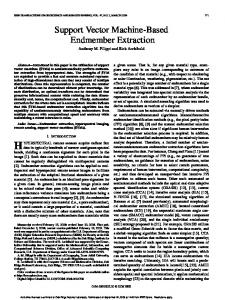
2. PROPOSED METHODOLOGY Let I1 and I2 be two co-registered multispectral images of size P×Q acquired over the same geographical area at different times t1 and t2. Let N be the number of spectral channels of each considered image and Ω = {ωn, ωc} the set of classes of unchanged and changed pixels to be identified. The proposed technique is based on a two-step procedure: i) an initialization step that exploits a Bayesian thresholding of the magnitude of SCVs; and ii) a Support Vector Data Description (SVDD) method that analyzes the multispectral difference image I∆ = I2 - I1 (see Fig. 1). Therefore, not only change information present in the magnitude of SVCs is considered, but also the high dimensional information present in the multispectral difference image. In the following, we analyze these steps in more detail.

I1

Initialization Vector difference

Magnitude operator

Iρ

Selective Bayesian Thresholding

ST, SO

SVDD Classifier Change Detection Map

I∆

I2

Fig. 1 Block scheme of the proposed system.

Proc. of SPIE Vol. 6748 674809-2

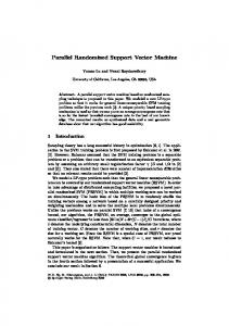
2.1 Bayesian Initialization The first step of the proposed unsupervised approach to change detection aims at identifying the sets ST and SO of target (unchanged pixels) and outlier (changed pixels) patterns to be used as seeds for initializing the support vector data description (SVDD) one-class classifier (OCC). Following the discussion in Ref. 5, these subsets should contain pixels that are associated with changed or unchanged areas on the ground. However, as in our problem no ground truth information is available, the ideal assumption is relaxed and replaced with the more realistic constraint that seeds included in the sets ST and SO are associated with a high probability to belong to changed or unchanged areas. According to the procedure described in Ref. 5, pixels with a high probability to belong to the change and no-change classes are identified by applying the CVA technique to I1 and I2, and by selectively thresholding the statistical distribution p(iρ) of the magnitude of SCVs in Iρ (iρ is the random variable associated with the magnitude of the spectral change vectors in Iρ). In the literature, several threshold-selection methods (e.g., see Ref. 3,9) have been proposed that can be used for identifying the threshold value T, which separates changed from unchanged pixels. Among them, we recall threshold-selection approaches based on the Bayesian decision theory, which showed to be effective in many change-detection scenarios. The application of the Bayesian theory to threshold selection requires the estimation of the class-statistical parameters, i.e., the class prior probabilities and the class-conditional probabilities. As we are dealing with an unsupervised change-detection problem, these statistical quantities are estimated from the data (without any prior information) according to the Expectation-Maximization (EM) algorithm.3 The estimated class-statistical parameters are then used with the Bayes decision rule for minimum error for identifying the decision threshold T that separates changed from unchanged patterns. However, if we apply the Bayesian threshold to Iρ, we obtain a change-detection map affected by the high uncertainty that characterizes patterns with a magnitude value close to the threshold. This problem arises from the loss of information associated with the magnitude operator. On the other hand, the threshold value T represents a reasonable reference point for identifying the subsets ST and SO. According to this observation and following Ref. 5, the desired sets of patterns with a high probability to be correctly assigned to one of the two classes are obtained by defining a margin around the minimum-error threshold. This margin conceptually separates uncertain from certain patterns. Patterns that fall outside the margin and show a high magnitude have a high probability to be changed pixels and are labeled as targets, whereas patterns that fall outside the margin and show a low magnitude have a high probability to be unchanged and are labeled as outliers. Therefore, the resulting sets ST and SO are defined as (see Fig. 2): ST = {x n ∈ℜ N | inρ ≥ T + δ 2 }n=1

P×Q

SO = {x n ∈ℜ N | inρ ≤ T − δ 2 }n=1

P×Q

and

(1)

where inρ is a 1-dimensional pattern in Iρ, and x n is a N- dimensional vector whose components are the spectral change vectors of the nth pattern in I∆. According to the standard classification setup, the n-th target pattern in ST is associated with a label yn = +1 whereas the nth outlier pattern in SO is associated with a label yn = −1 . It is worth noting that constants δ1 and δ2 should be selected in order to obtain a high probability that patterns in ST and SO are changed and unchanged, respectively.

p (i ρ ) SO

ST

δ1

δ2

T

iρ

Fig. 2 Example of distribution of the magnitude of SCVs p(iρ) and of definition of the targets and outliers subsets.

Proc. of SPIE Vol. 6748 674809-3

2.2 Change Detection based on SVDD with outlier information The second step of the proposed method aims at giving a description of the class of changed pixels (target) in the SCVs feature space by exploiting the information present in the target and outlier sets defined in the previous step. The higher dimensionality that characterizes the multispectral difference image allows integrating the incomplete information on targets and outliers extracted from the 1-dimensional magnitude of SCVs and achieving a better description of the target class. The problem of finding a description of the target class data is faced here by using a support vector data description (SVDD) technique.12,13 SVDD aims at distinguishing between targets and outliers defining a closed boundary around the target data.12,13 In greater detail, the SVDD defines a minimum volume hypersphere in the kernel space that includes all (or most) of the target patterns available in the training set by minimizing a cost function. Two different formulations of the cost function have been given in the literature. The first one involves only target examples in the definition of the cost function;12 whereas, the second one involves both targets and outliers.13 It has been shown13 that the joint use of both positive and negative examples in the training phase improves the data description. As in the considered data domain description problem it is possible to generate examples of both classes (as shown in the previous section), we adopt the second formulation for the definition of the minimum enclosing ball. Note that, depending on the size of the considered images, the cardinality of ST and SO can be high. To decrease the computational load, it is reasonable to randomly subsample both ST and SO. Therefore let us assume that after K subsampling the set of target pixels is made up of KT examples (i.e., ST = {xt }t =T1 ) whereas the set of outliers is made up of KO counterexamples (i.e., SO = {x o }o=O1 ). Following the notation in Ref. 13, let us assume that xo and xt in SO and ST, respectively, are column vectors. We can characterize the MEB with its center a and radius R (> 0), and define the problem of minimizing its volume as: K

2

min{R }

(1)

⎧⎪ φ ( x t ) − a 2 ≤ R 2 ∀t = 1, …, KT ⎨ 2 2 ⎪⎩ φ ( x o ) − a ≥ R ∀o = 1, …, K O

(2)

R ,a

subjected to

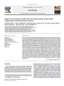
where φ (.) is a non-linear transformation that maps the data into a high dimensional Hilbert feature space H where targets data description can be achieved with a hypersphere. The first constraint in (2) comes from the assumption that positive examples should fall inside the sphere, while the second comes from the assumption that outliers should fall outside it (i.e., counterexamples should be rejected), see Fig. 3.

Hyperiphere in feature HilbertspaceH

• •

••

••

4'

4

Fig. 3 An example of hyperspherical boundary defined by SVDD: light grey samples (inside the sphere) are targets; and dark grey samples (outside the sphere) are outliers; and samples in the boundary are support vectors. Both target and outlier samples on the wrong side of the boundary are associated with slack variables to deal with errors.

Proc. of SPIE Vol. 6748 674809-4

As for standard SVMs, the cost function can be reformulated in order to allow a certain amount of errors in both the positive and negative samples sets. Let us introduce slack variables ξt (t = 1,…, Kt) and ξo (o = 1,…, Ko) associated with the target and outlier patterns, respectively (see Fig. 3). Accordingly, the error function to be minimized becomes:

⎧ R ,a ,ξt ,ξo ⎩

KT

KO

t =1

o =1

⎫ ⎭

min ⎨ R + CT ∑ ξ t + CO ∑ ξ o ⎬ 2

(3)

subjected to

⎧⎪ φ ( x t ) − a 2 ≤ R 2 + ξt , ξ t ≥ 0, ∀t = 1, …, K T ⎨ 2 2 ⎪⎩ φ ( x o ) − a ≥ R − ξ o , ξ o ≥ 0 ∀o = 1, …, K O

(4)

parameters CT and CO are two regularization parameters that control the trade-off between the volume of the hypersphere and the number of rejected patterns for the target and outlier classes, respectively. The primal function (3) is usually solved through its Lagrangian dual problem,13,19 which reduces to the solution of: KO KT ⎧ KT α φ ( x ), φ ( x ) − α φ ( x ), φ ( x ) − max ⎨ ∑ t ∑ o ∑ α tα u φ (xt ), φ ( xu ) t t o o α t ,α o ⎩ t =1 o =1 t ,u =1

(5)

⎫ +2 ∑ ∑ α oα p φ ( x o ), φ ( x p ) − ∑ α oα p φ ( x o ), φ ( x p ) ⎬ o =1 p =1 o , p =1 ⎭ K O KT

KO

constrained to KO

KT

∑ αt − ∑ αo = 1 t =1

o =1

KT

KO

t =1

o =1

a = ∑ α tφ ( xt ) − ∑ α oφ ( x o ) 0 ≤ α t ≤ CT ,

∀t = 1, …, KT

0 ≤ α o ≤ CO ,

∀o = 1, …, K O

(6)

The given data description always results in a closed boundary around the target class. The inner product of mapping functions φ (⋅) (which are in principle unknown) that appears in (5) can be replaced with a kernel function K (⋅, ⋅) : K ( x i , x j ) = φ ( x i ), φ ( x j )

with

i , j ∈ {o, t , p, u}

(7)

Substituting (7) into (5) we obtain

⎧ KT α t ,α o ⎩ t =1

KO

max ⎨ ∑ α t K ( x t , xt ) − ∑ α o K ( x o , x o ) − o =1

KT

K O KT

KO

t ,u =1

o =1 t =1

o , p =1

∑ α tα u K ( xt , xu ) + 2∑ ∑ α oα t K ( xo , xt ) − ∑

⎫ ⎭

α oα p K ( x o , x p ) ⎬

(8)

This allows us to construct a non-linear SVDD by defining only the kernel function, without needing to know the mapping φ (⋅) explicitly. After solving the dual problem, to decide whether any vector xn in I∆ belongs to the class of change (targets) or nochange (outliers) the distance to the center of the sphere should be evaluated. A pattern xn is classified as changed if it falls inside the sphere (i.e., its distance from the center of the sphere is lower than the radius), otherwise if the distance from the center of the sphere is higher than the radius, xn falls outside the boundary and it is marked as unchanged. The decision rules becomes as follows:

Proc. of SPIE Vol. 6748 674809-5

⎧⎪ωc

⇔

φ (x n ) − a

2

≤R

⎪⎩ωn

⇔

φ (xn ) − a

2

>R

xn ∈ ⎨

2

(9)

2

In other words, a vector xn is accepted as target if the following inequality is satisfied: φ ( x n )−a,φ ( x n ) −a = K ( x n , x n ) − 2

KO ⎡ KT ⎤ KT α K ( x n , x t ) − ∑ α o K ( x n , x o ) + ∑ α tα u K ( xt , x u ) ∑ t ⎢⎣ t =1 ⎥⎦ t ,u =1 o =1

KO KT

− 2∑ ∑ α oα t K ( x o , x t ) + o =1 t =1

KO

∑

o , p =1

α oα p K ( x o , x p ) ≤ R

(10)

2

otherwise it is rejected and identified as outlier.

3. EXPERIMENTAL RESULTS The proposed method has been tested on two multitemporal datasets made up of a pair of multispectral images acquired by the Thematic Mapper (TM) multispectral sensor of the Landsat 5 satellite. The first data set refers to an area in the Mexico, the second concerns the Sardinia Island (Italy). In the following subsections, we present the experimental setup and the results obtained on these data sets.

3.1 Experimental setup In all the experiments the initialization threshold value T was obtained according to a manual-trial-and-error procedure (MTEP). The use of this threshold leads to a change-detection map that shows the minimum overall error if compared to the reference map. This choice allowed us evaluating an “upper bound” of the performance of the proposed method without any bias due to human operator subjectivity or to the fact that the selection was made by an automatic thresholding algorithm. At an operational level, any automatic threshold-selection technique can be adopted (see Ref. 3 for more details about thresholding the magnitude image). The constants δ1 and δ2 were set equal to 10. In the learning of the SVDD three parameters should be defined: i) the width σ of the employed Gaussian kernel function10; ii) the regularization parameters CT for wrong pixels in the target class; and iii) the regularization parameters CO for wrong pixels in the outlier class. In our experiments, for convenience, we assumed that CT = CO. The modelselection was based on the available reference map according to a grid search strategy with values of the two free parameters in the following ranges: i) regularization parameters CT = CO = C ∈ [10−3 ,5] ; and ii) Gaussian kernel width σ ∈ [0.01,1] . The results obtained with the proposed method were compared with the ones obtained with a standard CVA algorithm applied to Iρ with manual trial-and-error thresholding procedure. The comparison is performed in terms of false alarms, missed alarms, overall errors and kappa coefficient of agreement evaluated according to the reference maps.

3.2 Results on the Mexico Data Set The Mexico data set is a section of 512×360 pixels of two co-registered multispectral images acquired by the TM sensor of the Landsat-5 satellite. The two images were acquired in April 2000 (I1) and May 2002 (I2) (Figs. 4 (a) and (b)). Between the two acquisitions, two wildfires occurred in this area. A reference map concerning their location was available (Fig. 4 (c)). This map includes 29506 changed pixels and 154814 unchanged pixels. A preliminary analysis pointed out that spectral channels 4 and 5 are the most relevant for discriminating the burned area on this data set. Accordingly, we used these channels in our trials. As can be seen from Fig. 5, this change-detection problem is a complex problem, as the target and outlier classes are significantly overlapped. In this critical situation the proposed technique resulted in higher change-detection accuracy than the standard technique (see Tab. 1). In greater detail, the proposed approach sharp increased the Kappa accuracy provided by the standard CVA from 0.844 to 0.9028. The improvement is associated to a sharp decrease of false alarms (from 3840 to 2031) and to a slight reduction of missed alarms (from 3879 to 3141).

Proc. of SPIE Vol. 6748 674809-6

(a) (b) (c) Fig. 4 Channel 4 of the Landsat-5 TM Images acquired on the Mexico in: (a) April 2000, and (b) May 2002. (c) Available reference map of the burned areas.

Numerical results are confirmed also by a qualitative comparison of the two change-detection maps reported in Fig. 6. As can be seen, the map obtained with the proposed technique shows less isolated changed pixels with respect to the map yielded with the CVA. Pixels affected by registration noise result in a high magnitude as changed pixels do, but they show different SCVs components, therefore they are properly classified as outliers in the higher dimensional feature space of the multispectral difference image, whereas they are not in the magnitude domain. Therefore, burned areas are better identified confirming the effectiveness of the proposed approach. Table 1 False alarms, missed alarms, overall errors and Kappa coefficient for the change detection maps obtained for identifying the burned areas (Mexico data set). Technique CVA Proposed

Missed Alarms False Alarms Overall Error Kappa Accuracy 3879 3840 7719 0.8440 3141 2031 5172 0.9028

/,

0.8 0.7 0.8 0.8 0.4 0.3

02

0

0

DI

02

03 04 08 08 07 08 08

Fig. 5 Distribution of the class of changed (dark grey) and unchanged (light grey) pixels in the 2-dimensional I∆ image according to the available reference map. The black line is the SVDD decision boundary (Mexico data set).

Proc. of SPIE Vol. 6748 674809-7

--

-

.. I,

(a) (b) Fig. 6 Change-detection maps obtained for the Mexico data set: (a) standard CVA; and (b) proposed technique.

3.3 Results on the Sardinia Data Set The second data set is made up of two multispectral co-registered images acquired by the Thematic Mapper (TM) multispectral sensor of the Landsat 5 satellite on the Island of Sardinia (Italy) in September 1995 (I1) and July 1996 (I2). A section of 412×300 pixels was selected for the experiments including Lake Mulargia. As an example of the images used in the experiments, Figs. 7 (a) and (b) show channel 4 of the September and July images, respectively. Between the two acquisition dates the lake surface registered an enlargement of the water surface resulting in a spectral change. A reference map of the analyzed site was defined according to a detailed visual analysis of both the available multitemporal images and the difference image. The obtained reference map contains 7480 changed pixels and 116120 unchanged pixels (see Fig. 7 (c)). In the experiments, we considered only the two spectral channels 4 and 7 of the TM, i.e. the near and the middle infrared, as they are the most reliable for detecting changed areas.

(a) (b) (c) Fig. 7 Images of the Lake Mulargia (Italy). (a) Channel 4 of the Landsat-5 TM image acquired in September 1995; (b) Channel 4 of the Landsat-5 TM image acquired in July 1996; (c) available reference map of changed areas.

In remote sensing images, the spectral signature of the water class significantly differs from the spectral signatures of all other natural classes. For this reason, SCVs associated with changes in the water class show smaller overlapping to unchanged SCVs than in the previous case in both the Iρ and I∆ images (see Fig. 8). Therefore detection of changes associated to the appearance (or disappearance) of water becomes a relatively simple problem. Under these conditions, the standard CVA performs well resulting in a high Kappa accuracy (i.e., 0.95) which is a result difficult to improve. Therefore, as expected, the proposed technique results in a similar Kappa accuracy (see Table 2). Nonetheless, it is worth observing that also in this case the CVA resulted in a slightly larger amount of false alarms (i.e., 369) than the proposed technique (i.e., 295). This behavior is related to the higher sensitivity of the standard CVA technique to the presence of residual noise.

Proc. of SPIE Vol. 6748 674809-8

Table 2 False alarms, missed alarms, overall errors and Kappa coefficient for the change detection maps obtained for identifying the burned areas (Sardinia data set). Missed Alarms False Alarms Overall Error Kappa statistic 335 369 704 0.9500 373 295 668 0.9527

••tr

*4

Technique CVA Proposed

Fig. 8 Distribution of the class of changed (dark grey color) and unchanged (light grey color) pixels in the 2-dimensional I∆ image according to the available reference map. The black line is the SVDD decision boundary (Sardinia data set).

4. DISCUSSION In this paper, a novel approach to unsupervised change detection based on CVA and SVDD has been proposed. The proposed method formulates the change-detection problem as a minimum enclosing ball problem with changed pixels as target objects. The MEB problem is solved after mapping spectral change vectors into a high dimensional Hilbert space. Once the minimum volume hypersphere is computed, it is mapped back into the original feature space where it results in a non-linear flexible boundary around target pixels. With respect to standard change vector analysis that considers only the 1-dimensional magnitude of SCVs, the proposed techniques takes advantage from the higher amount of information present in the multidimensional SCVs feature space. This results in a better identification of changed areas, particularly in problems with overlapping classes. Furthermore, focusing on the changed pixels, it allows reducing the impact of residual registration noise in the final change-detection map. As future developments of the proposed work we propose: i) to introduce in the system architecture an approach for performing the model selection of the SVDD in a complete unsupervised way; and ii) to define a semi-supervised strategy for the learning of the SVDD parameters in order involve in the SVDD learning phase also unlabeled pixels according to the cluster assumption.

ACKNOWLEDGMENTS This paper has been partially supported by the Italian and Spanish Ministries for Education and Science under grant ``Integrated Action Programme Italy-Spain''.

Proc. of SPIE Vol. 6748 674809-9

REFERENCES 1

2 3 4 5 6

7

8 9

10 11 12 13 14

15 16 17 18 19 20

A. Singh, “Digital change detection techniques using remotely-sensed data.” Int. J. Remote sensing, 10, 989-1003 (1989). F. Bovolo and L. Bruzzone, “A theoretical framework for unsupervised change detection based on change vector analysis in polar domain,” IEEE Trans. Geosci. Rem. Sens. 45(1), 218-236 (2007). L. Bruzzone, D. Fernández Prieto, “Automatic analysis of the difference image for unsupervised change detection”, IEEE Trans. Geosci. Rem. Sens., 38, 1171-1182 (2000). F. Bovolo and L. Bruzzone, “Unsupervised change detection in multitemporal SAR images,” in Signal and Image Processing for Remote Sensing, Washington, DC: Taylor & Francis, Ed: C. Chen (2006). F. Bovolo, L. Bruzzone and M. Marconcini, “An Unsupervised Change Detection Technique Based on Bayesian Initialization and Semisupervised SVM,” IEEE Int. Geosci. Rem. Sens. Symp. (IGRSS), Barcelona, Spain (2007). F. Bovolo and L. Bruzzone, “A Split-Based Approach to Unsupervised Change Detection in Large-Size Multitemporal Images: Application to Tsunami-Damage Assessment,” IEEE Trans. Geosci. Rem. Sens. 45(6), 16581670 (2007). S. Ghosh, L. Bruzzone, S. Patra, F. Bovolo, and A. Ghosh, “A Context-Sensitive Technique for Unsupervised Change Detection Based on Hopfield-Type Neural Networks,” IEEE Trans. Geosci. Rem. Sens. 45(3) 778-789 (2007). F. Bovolo and L. Bruzzone, “A detail-preserving scale-driven approach to change detection in multitemporal SAR images,” IEEE Trans. Geosci. Rem. Sens. 43(12), 2963 – 2972 (2005). Y. Bazi, L. Bruzzone, and F. Melgani, “An unsupervised approach based on the generalized Gaussian model to automatic change detection in multitemporal SAR images,” IEEE Trans. Geosci. Remote Sens., 43(4), 874-887 (2005). G. Ritter and M.T. Gallegos, “Outliers in statistical pattern recognition and an application to automatic chromosome classification,” Pattern Recognition Letters, 18, 525-539 (1997). L. Tarassenko, “Novelty detection for the identification of masses in mammograms”, Proc. 4th IEE Int. Conf. Artificial Neural Networks, 4, 442-447 (1995). D. Tax and R. P. Duin, “Support vector domain description,” Pattern Recognition Letters 20, 1191–1199 (1999). D. Tax and R. P. Duin, “Support vector data description,” Machine Learning, 54, 45-66 (2004). G. Camps-Valls, L. Gomez-Chova, J. Muñoz-Marí, L. Alonso, J. Calpe-Maravilla, and J. Moreno, “Multitemporal image classification and change detection with kernels,” in SPIE International Symposium Remote Sensing XII, 6365, Stockholm, Sweden, (2006). J. Muñoz-Marí, L. Bruzzone, and G. Camps-Valls, “Evaluation of one-class domain description methods in remote sensing data classification,” IEEE Trans. Geosci. Rem. Sens., 8, 2683-2692 (2007). B. Schölkopf, R. C. Williamson, A. Smola, and J. Shawe-Taylor, “Support vector method for novelty detection,” in Advances in Neural Information Processing Systems 12, NIPS , Denver, CO (1999). G. Camps-Valls, J. L. Rojo-Álvarez and M. Martínez-Ramón, Kernel Methods in Bioengineering, Signal and Image Processing. Idea Group Inc. (2006), Harshey, PA (USA). J. Shawe-Taylor and N. Cristianini, Kernel Methods for Pattern Analysis, Cambridge University Press (2004). B. Schölkopf and A. Smola, Learning with kernels-support vector machines, regularization, optimization and beyond. MIT Press (2002). A. Ben-Hur, D. Horn, H.T. Siegelmann, and V. Vapnik, “Support Vector Clustering,” J. Machine Learning Research, 2, 125-137 (2001).

Proc. of SPIE Vol. 6748 674809-10