Anisotropic Volume Rendering for Extremely Dense, Thin ... - CiteSeerX

Anisotropic Volume Rendering for Extremely Dense, Thin Line Data Greg Schussman∗ Stanford Linear Accelerator Center

Abstract Many large scale physics-based simulations which take place on PC clusters or supercomputers produce huge amounts of data including vector fields. While these vector data such as electromagnetic fields, fluid flow fields, or particle paths can be represented by lines, the sheer number of the lines overwhelms the memory and computation capability of a high-end PC used for visualization. Further, very dense or intertwined lines, rendered with traditional visualization techniques, can produce unintelligible results with unclear depth relationships between the lines and no sense of global structure. Our approach is to apply a lighting model to the lines and sample them into an anisotropic voxel representation based on spherical harmonics as a preprocessing step. Then we evaluate and render these voxels for a given view using traditional volume rendering. For extremely large line based datasets, conversion to anisotropic voxels reduces the overall storage and rendering for O(n) lines to O(1) with a large constant that is still small enough to allow meaningful visualization of the entire dataset at nearly interactive rates on a single commodity PC.

Kwan-Liu Ma† University of California at Davis visualization of very dense particle paths from the simulation of particle accelerator structures. Even in the 2D case, the paths become a tangled mess long before global patterns emerge. Another source of line data results from integrating a very large number of streamlines through CFD data to capture intricate structural details in velocity and vorticity fields. The visualization challenge is to convey, clearly and interactively, the global structure of the dark current particle paths, or to show their relationship with electric and magnetic fields. This is a more difficult problem than simple vector field visualization because each point in a vector field maps to exactly one vector, but for path data, a point may map to any number of paths. For vector field visualization using streamlines, the line density can be adjusted by changing the number and placement of seed points. However, for measured or simulated path data, all paths are potentially significant so no path can be automatically discarded to reduce path density.

Keywords: anisotropic lighting, line data, scientific visualization, vector field, volume rendering

This paper presents Anisotropic Volume Rendering (AVR), a new technique making possible the depiction of extremely dense, fine field lines. Our basic approach is to subdivide the region of interest into cubes, which have their line data sampled and converted into voxels with anisotropic radiance and opacity. Voxels are represented efficiently by non-linear approximation where only significant spherical harmonics coefficients from a truncated Laplace series are stored. Direct volume rendering is then performed on traditional voxels computed from the anisotropic voxels, each evaluated according to a given viewing direction. Interactive scaling of line thickness is possible. The resulting voxel data size has a fixed upper bound, thereby enabling an overview of extremely large data on a commodity PC.

1

2

CR Categories: I.3.3 [Computer Graphics]: Picture/Image Generation; I.3.7 [Computer Graphics]: ThreeDimensional Graphics and Realism; I.4.10 [Image Processing]: Image Representation—Volumetric.

Introduction

Many scientific investigations require the study of complex 3D or 4D vector fields such as fluid flow field, electric field, and magnetic field. Displaying the field lines directly is popular. However, when the field consists of a large number of dense, intertwined lines, it becomes very difficult to depict the spatial relationships between the lines and their intrinsic global and local structures. For example, one problem, known as the dark current problem, under study by the scientists at the Stanford Linear Accelerator Center (SLAC) for the design of National Linear Collider (NLC) requires ∗ [email protected] † [email protected],

http://www.cs.ucdavis.edu/˜ma

IEEE Visualization 2004 October 10-15, Austin, Texas, USA 0-7803-8788-0/04/$20.00 ©2004 IEEE

Previous Work

Spherical harmonics were first introduced into computer graphics in 1987 for representing bidirectional reflection functions from surface bump maps [Cabral et al. 1987]. In general, they are useful for sampling and reconstructing a scalar function on a sphere [Glassner 1995]. In particular, they have been used for representing BRDFs for material surfaces and directional intensity distributions for surfaces [Sillion et al. 1991] and, more recently, for real-time rendering using complex environment maps converted into the frequency domain [Ramamoorthi and Hanrahan 2001]. One approach to anisotropic function representation uses a nonlinear (discarding insignificant coefficients) wavelet lighting approximation [Ng et al. 2003] to be faster than linear spherical harmonics. However, one can obtain speed increases by discarding insignificant spherical harmonic coefficients in a similar way, which is what we do. So in the same sense, our approach would be classified as using a non-linear Laplace Series approximation. The use of spherical harmonics for capturing anisotropy has so far been limited to one-sided surfaces [Ramamoorthi and Hanrahan 2001; Sloan et al. 2002; Ng et al. 2003]. The illuminated line work most closely related to ours is that by [Stalling et al. 1997]. Their work uses 2D textures of precomputed illumination based on the work of [Banks 1994], which treats lines as 1-manifolds in 3-space. A consequence

107

of this is that, for any point on the curve, there is no clear surface and therefore no clear surface normal vector (rather, there are an infinite number of surface normals which are constrained to a plane). The diffuse term for the shading equation suffers from “excess brightness” which can be alleviated by exponentiating that term. Although values for this exponent are presented, we have found that some manual adjustment is needed in practice. Line primitives have some additional drawbacks. They do not provide the perspective depth cue. For extremely dense sets of lines, transparency is needed to prevent the rendering of an opaque mass. But transparency introduces its own set of difficulties. Limited precision in graphics hardware can cause severe quantization error for very transparent lines. Transparency also calls for back-to-front compositing of the line fragments, but this sorting can be prohibitively expensive for extremely large datasets. It is pointed out by [Stalling et al. 1997] that back-to-front compositing of approximately sorted segments (by an individual axis) yields only about 1% pixels with somewhat incorrect color, and that display lists of pre-sorted lines (along the major axes) speeds rendering. However line datasets too large to fit in memory preclude storing multiple sorted copies and the use of display lists. Furthermore, for very dense lines, approximate sorting can result in significant visual artifacts. Our approach is more closely related to what Banks refers to as promoting the manifold dimension; that is, we treat curves as tubes, so that normal vectors are cleanly defined, and there is a real surface with a visible side over which to integrate a shading equation. However our goal is to handle tubes projecting to have sub-pixel widths (consistent with averaging down a supersampling of shaded geometric tubes), so these integrated values are accumulated into floating point spherical harmonics coefficients for anisotropic voxels. This provides sub-pixel illumination consistent with multi-pixel illumination, correct depth ordering (except within an individual voxel), a fixed upper bound on memory requirements regardless of the line data size, and provides the perspective depth cue if the volume renderer renders in perspective. This also accumulates all line contributions to a voxel prior to entering graphics hardware, so that an individual voxel is not subject to accumulated quantization error in hardware. Volume haloing [Interrante and Grosch 1998], which requires more than one pixel of projected tube thickness, is not appropriate for what we intend to accomplish. The work most closely related to the volumetric aspect of ours uses three dimensional textures to render fur [Kajiya and Kay July 1989], and mentions the desirability of the Painter’s Illusion in which far more detail is suggested than is actually present on very close examination of a region of an image. Toward this end, they model teddy bear fur as a dense block, and tile this over the surface of the bear. The diffuse component of their lighting model is essentially the same as ours, but their specular model assumes uniformly dense fur and diffraction, which is not appropriate for the highly non-uniform density datasets which motivated AVR. They mention that the specular contribution can be derived using an approach similar to the diffuse contribution, but they admit that doing so is difficult and results in a model which is “quite complex”. A contribution of this paper is an efficiently computable, nearly analytical solution to this specular problem. Their representation is based on storing a density, a frame, and a reflectance function, where the reflectance function is common to the whole dataset. In contrast, the AVR representation uses Laplace Series coefficients to store anisotropic density and radiance, with the frame assumed to be common to the whole dataset. Their approach makes numerous assumptions about the teddy bear fur, but these do not hold for scientific datasets. The AVR approach only assumes that the fiber thickness is smaller than the voxel dimensions. Finally, they use ray tracing to producing nice shadowing effects during rendering. If global illumination were to be used with AVR, it would occur during pre-

108

processing, but could then be rendered as quickly as other lighting models. Light transport and illumination of micro geometry has also been an area of graphics research. In the work of [Daubert et al. 2003] visibility and illumination are precomputed for tiled repetitive micro-geometry by raycasting a tile. This allows efficient rendering with global illumination, but the preprocessing method is prohibitively expensive because our datasets are much larger and do not contain tiled repetitive patterns. By restricting our micro-geometry to tubes and using a nearly analytical function for precomputation of local illumination and occlusion for tubes, we are able to preprocess very large datasets in a fraction of the time that they take to generate. The work of [Sillion et al. 1991] also considers micro-geometry, but assumes the overall reflection properties do not vary over a surface. Recent research has also been done on light scattering from human hair [Marschner et al. 2003] where the hair is not opaque and light undergoes multiple scattering within a fiber. Their goal is match the visual qualities of real hair. In contrast, our goal is to match opaque supersampled tube geometry illuminated with a given shading model. We want a visual match for tubes so thin that supersampling is intractable (e.g., for sets of fibers which are orders of magnitude thinner and denser than human hair).

3

Anisotropic Volume Rendering

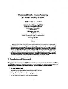
The AVR process, illustrated in Figure 1, consists of two phases, one for preprocessing, and the other for rendering. A traditional voxel has only an opacity and color, which are isotropic (independent of viewing direction). An AVR voxel has opacity and color intensity, but these are anisotropic.

Figure 1: Flowchart of AVR preprocessing (left) and rendering (right). The input for AVR consists of line data, where these lines or curves are represented as line segments. Each segment has a beginning and an ending point in 3D, and an associated radius and material properties. The first step in preprocessing is to partition the (presumably gigantic) line dataset into blocks which are of manageable size. Because the input data is too large to fit in memory, and the number of blocks to be saved can exceed the maximum allowable number of open files, we buffer the line segments in memory, and only

~ L

open and append to a file when more than a certain number of segments have accumulated for the corresponding block. This allows all line data to be partitioned in a single streaming pass without incurring significant penalty for opening and closing files. Once the data has been partitioned into blocks, the blocks can be voxelized in an embarrassingly parallel fashion. Voxelization consists of clipping line segments to voxel boundaries and accumulating spherical harmonic coefficients. Clipping is straightforward; each block corresponds to an n3 volume of voxels, so every line segment is clipped to the cubical boundaries of any voxel region through which it passes. The Laplace Series coefficients are then computed for the lighting contribution of the clipped subsegment, and accumulated in the corresponding AVR voxel. Lighting can be from multiple light sources, which can be any mixture of ambient and directional light sources, and the directional light sources can be either fixed in world space (e.g., the sun) or fixed in eye space (e.g., a headlight). Once all segments have been processed, insignificant coefficients are discarded. The details of these calculations are presented in Section 4. The final output of the preprocessed data is blocks of AVR voxels. In our implementation, each block is a 3D array of pointers which are null for empty (completely transparent) voxels, or point to an instance of an AVR voxel class. Each block stores the indices for its location within the entire volume, and thereby can “know” where it is located in 3D. An AVR voxel consists of a list of quantum numbers and an associated list of coefficients. Because these coefficients are accumulated in software, no quantization error is introduced prior to hardware rendering. If the addition were done in limited precision graphics hardware, a dense bundle of fine lines could have each individual line quantized to 0, even though collectively the bundle should be visible. The rendering phase takes as input blocks of AVR voxels, the eye position and viewing direction of an observer, and other viewing parameters such as transfer functions. These are used to evaluate a block of AVR voxels. When an AVR voxel is evaluated, the input is a viewing direction, and the output is an rgb color intensity and an opacity value. In effect, evaluating a block of AVR voxels produces a block of traditional voxels corresponding to the current view. Traditional volume rendering can then be performed in parallel to produce sub images which are composited to produce a final image. The opacity of AVR voxels is directly proportional to the corresponding segment radii, so the equivalent of interactively scaling the radii can be accomplished by scaling the opacity of an evaluated AVR voxel. If there are more than one input line type (for example electric field lines and magnetic field lines), these can be preprocessed independently, and can have their evaluated results scaled and combined interactively, also without further preprocessing. Opacity transfer functions can also be manipulated once the AVR voxel opacity has been evaluated.

4

Averaged Lighting Derivations

This section provides the mathematical details for implementation. There are two steps in execution. The first is to compute the averaged lighting for a single line segment from a single view with a single light source. This is repeated for any additional segments lying within the current voxel. This would also be repeated for additional light sources. For this specific view, the color and opacity are accumulated via a weighted average. The organization for this section is as follows. First we state

l

T~

r

T~

(a)

~ V (b)

Figure 2: Each segment has a radius r, length l, and unit tangent vector T~ (a). Input unit vectors consist of T~ , the ~ and view V ~ (b). light source L,

our assumptions and conventions, and describe our notation. Then we provide a starting point for deriving expressions for averaged lighting contribution of a generic light source which can be any shading function. This starting point is an integral for which an efficiently computable analytical or numerical solution is needed to make preprocessing of large datasets tractable. Next, special limits of integration for the specific case of a directional light source are given, followed by the weighted averaging equations for color and opacity. This section concludes with the solution of the averaged lighting integrals for the specific case of OpenGL’s Phong style lighting model.

4.1

Conventions and Notation

First, we make some simplifying assumptions. The mathematical formulation of intensity (as a function of view direction, curve tangent, and light direction) assumes orthographic projection during sampling. However, during visualization, the overall view uses perspective projection, and permits up-close viewing. The derivations in this section assume that the radius of any cylinder is less than the width of the surrounding voxel. The relative depth relationship of two line segments is not preserved within the same voxel but is preserved between separate voxels. ~ a view vecLighting parameters consist of a light vector, L, ~ , and light properties. Lines (curves) are composed of tor, V line segments which are modeled as cylinders. Each cylinder has radius r, and length l. A cylinder has material properties: ambient, diffuse, and specular coefficients for red, green, and blue color channels, and a shininess exponent. A unit vector T~ , which lies along the axis of the cylinder, can be thought of as a normalized version of the average tangent vector for this cylinder’s portion of the curve. Figure 2a shows these cylinder parameters in relation to one another. ~ and L ~ points toward the eye and a disThe unit vectors V tant light source, respectively, and are depicted in Figure 2b in relation to T~ . ~ . DisWe construct a 3D orthogonal basis from T~ and V regarding the special case where a cylinder is viewed “end on” (because there would be no visual contribution), T~ and ~ are linearly independent, and the orthogonal projection V ~ into the plane perpendicular to T~ is the unique vecof V ˛ ˛ ~p where 0 < ˛˛V ~p ˛˛ ≤ 1. The three basis vectors are T~ , tor V ~ , and B ~ N the latter two are “computed “ where ” ” according to ~ ~p , B ~ = T~ × N ~, V ~p = V ~ − V ~ · T~ T~ , where N deN =N V

~B ~ plane is perpendicular notes vector normalization. The N ~ to the T axis, effectively forming a cross-sectional slice of the ~ is the cylinder surface cylinder from Figure 2b. Note that N

109

normal which most closely points toward the eye. We define any other unit surface normal in terms of the angle θ, which ~B ~ plane, going clockwise about the is the rotation in the N T~ axis, so ~ cos θ + B ~ sin θ. ~n(θ) = N (1) The projected visible side of the cylinder corresponds to − π2 ≤ θ ≤ π2 .

4.2

Generic Initial Derivation

The initial portion of derivations for averaged lighting over a cylinder surface have a common starting point independent of the expression for the light source. Using F as a generic placeholder for a light contribution from any shading model, the generic averaged intensity, I¯F , is the shading intensity integrated over the projected visible cylinder surface divided by the projected area of the cylinder surface: Z . I¯F = F cos φ dSV L Areavis , (2)

4.3

Weighted Average within a Voxel

Averaged lighting expressions from Section 4.2 provide the lighting contribution of a single cylinder for a given view. This paper targets extremely dense line datasets where many line segments can lie within a single AVR voxel. We use a weighted average to combine the contributions of multiple segments for this view. For n cylinders numbered i ∈ {0, 1, . . . , n − 1}, we denote the rgb color triplet by Ci , the projected visible area (as computed in Equation 3) by Ai , and the final color and opacity for a voxel by C and O, respectively. The weighted averages are ,n−1 n−1 X X C = (Ci )(Ai ) Ai , (6) i=0

O

=

1−

i=0

n−1 Y„ i=0

1 − Ai

.S « c

4

.

(7)

where Sc is the surface area of the cube, and Sc /4 is the average visible surface area of a cube [Arvo and Kirk 1989].

SV L

Here, SV L denotes the projected area that is both visible and illuminated. Note that SV L depends on F, and that SV L ⊆ S, because S denotes all projected visible area, regardless of whether that area is illuminated. The limits of integration for θ (corresponding to SV L ) are not necessarily −π and π2 , 2 and depend on what F is. The projected visible area of a cylinder surface is “ ” ~ ·N ~ . Areavis = 2 rl V (3) Equation 2 can be partially evaluated, taking Equation 3 into account and using dS = r dθ dz from cylindrical coordinates. The simplified resulting expression concludes the initial derivation, and is now ready to accept F: Z θ1 I¯F = 21 F cos θ dθ. (4) θ0

The limits of integration for θ for the cylinder surface which is both visible to the eye and illuminated by a directional ~p denotes light source are illustrated in Figure 3, in which V ~ into the N ~B ~ plane, L ~ p denotes the prothe projection of V ~ into the N ~B ~ plane, and α is the angle between jection of L the projected view and projected light vectors. From this figure, the limits of integration for a directional light source are ` ´ ` ´ θ0 = max −π , α − π2 , θ1 = min π2 , α + π2 . (5) 2 ~ B

~ B

π 2

α+ π 2

0 −π 2

~p N ~ V

~ B

~p L α− π 2

θ1

α

~ N

~ N θ0

Figure 3: The portion of the cylinder surface visible to the eye (left) may not be the same as the portion of the surface illuminated (middle). Integrating only over the intersection of these two regions (right) simplifies the sampling equations for directional light sources.

110

4.4

Application to OpenGL Lighting

The mathematics of OpenGL’s lighting are given in Chapter 5 of the OpenGL Programming Guide (the “Red Book”) [Woo et al. 1999]. To summarize briefly, OpenGL uses the following (in slightly different notation) to produce the color I = Ia + Id + Is where I is the total intensity rgbα vector, and the a, d, and s subscripts correspond to ambient, diffuse, and specular, respectively. Denoting componentwise vector multiplication by ∗, Ia

=

Id

=

Is

=

(Am ∗ Al ),

“ ” ~ · ~n, 0 , (Dm ∗ Dl ) max L “ ”k ~ · ~n, 0 , (Sm ∗ Sl ) max H

(8) (9) (10)

where ~n is the surface normal vector, A, D, and S correspond to ambient, diffuse, and specular, respectively. The subscripts m and l correspond to material and “ light,”respec~ +V ~ . ~ =N L tively. The “halfway” unit vector is H

In this case, the average intensity I¯ = I¯a + I¯d + I¯s . The individual sub-expressions come from substituting Equations 8, 9, and 10 in place of F in Equation 4. The ambient term is simply I¯a = Am Al , and the easily obtained simplified diffuse term is »“ ”“ ” ~ ·N ~ sin 2θ1 − sin 2θ0 + 2(θ1 − θ0 ) L I¯d = Dm8Dl (11) “ ”“ ”– ~ ·B ~ cos 2θ1 − cos 2θ0 . − L Space constraints preclude showing the complete derivations here, but they are available in [Schussman 2003]. The specular expression is more challenging, so we provide a summarized derivation here. The main difficulty surrounding integration of the specular expression is the k exponent, which causes analytical solutions (for known k) to expand out to so many trigonometric terms as to be computationally impractical (even for preprocessing large datasets). Starting with Equation 4, and using F = Is from Equa-

tion 10 gives I¯s =

1 2

Z

θ1

Sm Sl θ0

“

~ · ~n(θ) H

”k

cos θ dθ.

(12)

Substituting Equation 1 into Equation 12, and distributing the dot product yields Z θ1 h“ ” “ ” ik ~ ·N ~ cos θ+ H ~ ·B ~ sin θ cos θ dθ. (13) I¯s = Sm Sl H 2

θ0

We now rearrange and split up this expression so that the part which does not have an analytical solution will at least lend itself to a precomputed numerical solution. Toward this ~ p and β; similar to L ~ and L ~ p in Figure 3, end, we introduce H ~ ~ ~ ~ Hp is the projection of H into the N B plane, so “ ” “ ” ~p = H ~ ·N ~ N ~ + H ~ ·B ~ B, ~ H (14)

~ p and the N ~ axis, which can be and β is the angle between“H ” ~ p ) · B, ~ N (H ~ p) · N ~ , where computed as: β = atan2 N (H atan2 is ISO 9899 ˛ ˛ compliant. The orthogonal projection of ˛~ ˛ ~ ~ ~ ~ Hp onto N is ˛H p ˛ cos β. Because Hp and H both have the ~ and B ~ components, the following equations result: same N ˛ ˛ ˛ ˛ ~ ·N ~ = ˛˛H ~ p ˛˛ cos β, ~ ·B ~ = ˛˛H ~ p ˛˛ sin β. H H (15) Substituting these into Equation 13, then substituting in a trigonometric angle addition identity, and using a change of variables where u = θ − β, and using another angle addition identity gives Z θ1 +β ˛ ˛k−1 “ ˛~ ˛ ~ ·N ~) I¯s = Sm2Sl ˛H (H cosk+1 u du p˛ θ0 +β

~ · B) ~ −(H

Z

θ1 +β

θ0 +β

(16)

” cos u sin u du . k

The second integral in Equation 16 has a clean, closed-form solution, but the first integral does not. The integral of cosk+1 u is an order k multivariate polynomial in cos u and sin u with k + 2 terms for even k, or k + 1 terms for odd k. If u is bounded below and above, (which we denote by umin and umax , respectively), the integral can be precomputed numerically and stored in a lookup table. From our change of variable and we obtain bounds for β, and then substitute back to get umin = −π ≤ u = (θ − β) ≤ π = umax . Because these bounds exist, a function F (u0 , u1 ), implemented in terms of the lookup table, can be used to replace the problematic integral, providing our final expression for the averaged specular contribution: ˛ ˛k−1 »“ ” ˛~ ˛ ~ ·N ~ F (θ0 + β, θ1 + β)+ I¯s = 21 Sm Sl ˛H H p˛ “

” „ cosk+1 (θ − β) − cosk+1 (θ − β) «– 1 0 ~ ~ H ·B , k+1

The sampling function only takes a view, a cylinder and a light source. It can be called multiple times, once for each light source, and the results can be combined. Light sources can have any direction, either held fixed in world space, or held fixed in eye space, or defined as some other function of viewing direction. Samples from different cylinders within the same voxel are combined as well. Once the compact representation is obtained, sampling need not be repeated unless the combined lighting functions are changed (examples include light sources being added or removed, a world space light being moved in world space, or a light direction being redefined as a different function of viewing direction). Spherical harmonic functions form the basis for the Laplace series in a way that is directly analogous to sine and cosine harmonics forming the basis for Fourier series. We adopt the spherical coordinates convention most commonly used in physics, as follows. The azimuthal angle, φ, lies in the XY plane, is measured from the X axis, is confined to the interval [0, 2π], and corresponds to longitude. The polar angle, θ, is measured from the Z axis, is confined to the interval [0, π], and corresponds to colatitude (where colatitude is 90◦ −latitude). Cartesian coordinates are obtained from spherical coordinates as (x, y, z) = (sin θ cos φ, sin θ sin φ, cos θ). The normalized spherical harmonics are typically denoted by Yl,m and defined in real form by 8 m>0 < Nl,m Pl,m cos θ , cos √ mφ, Yl,m (θ, φ) = Nl,0 Pl,0 (cos θ) / 2, m = 0 , (18) : Nl,m Pl,|m| (cos θ) sin |m| φ , m