Data-Parallel Volume Rendering Algorithms - CiteSeerX

1

Data-Parallel Volume Rendering Algorithms Roni Yagel and Raghu Machiraju Department of Computer and Information Science The Ohio State University Images generated from volumetric datasets are increasingly being used in many biomedical disciplines, archeology, geology, high energy physics, computational chemistry, computational fluid dynamics, meteorology, astronomy, computer aided design, environmental sciences, and many others. However, given the overwhelming amounts of computations required for accurate manipulation and rendering of 3D rasters, it is obvious that special purpose hardware, parallel processing or a combination of both are imperative. In this presentation we consider the image composition scheme for parallel volume rendering in which each processor is assigned a portion of the volume. A processor renders only its data by using any existing volume rendering algorithm. We describe one such parallel algorithm that also takes advantage of vector processing capabilities. The resulting images from all processors are then combined (composited) in visibility order to form the final image. The major advantage of this approach is that, as viewing and shading parameters change, only 2D partial images are communicated among processors and not 3D volume data. Through experimental results and performance analysis we show that our parallel algorithm is amenable to extremely efficient implementations on distributed memory MIMD (Multiple Instruction Multiple Data) vector-processor architectures. It is also very suitable for hardware implementation based on image composition architectures, it supports various volume rendering algorithms, and it can be extended to provide load-balanced execution and to support rendering of unstructured grids.

1. Introduction The last decade saw the rapid increase in the use of volumetric data in a growing number of disciplines due mainly to the enhanced capacity and power of affordable computers. Volumes are the natural extension of 2D rasters to the third dimension. In their simplest form, volumes are defined as a 3D raster made of small cubic cells (voxels) each representing a unit of space. The same way a pixel can hold a digital representation of an area unit, a voxel stores a collection of attributes pertaining to a unit of space. These attributes may consist of, for example, a scalar value representing material density or a vector representing flow direction. Biomedical applications have pioneered the utilization of volumes to represent and render data collected by a plethora of new acquisition technologies such as Computed Tomography (CT), Magnetic Resonance Imaging (MRI), Ultrasound, and others. Images generated from such datasets are being clinically used, across all the medical disciplines, in diagnosis, treatment planning, delivery of treatment, and the assessment of its effectivity. Many other disciplines in science and industry have joined this trend. Among the many examples are archeology,

2

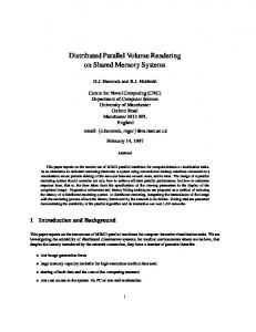
geology, high energy physics, computational chemistry, computational fluid dynamics (CFD), meteorology, astronomy, computer aided design (CAD), and environmental sciences. Direct volume rendering is now considered a viable method for visualizing volumetric scalar fields. The scalar field value assigned to each voxel can represent the tissue density as measured by CT machines, the pressure in a fluid as computed by CFD simulators, or an object tag as derived from 3D scan-conversion or voxelization of geometric objects. In direct volume rendering each voxel is first ascribed material and visual properties such as color, opacity, or reflectivity. This application dependent process is based on the classification of the raw data into displayable materials. We will assume that the volumes we deal with have been classified. Volumes can be obtained from sampling a real valued scalar function in three dimensional space at discrete grid points. Since the rendering process involves resampling, in order to reduce artifacts in the final image, the original function should be reconstructed before rendering. In the second phase of the rendering process, given user controlled viewing parameters (e.g., eye position, viewing direction), the data is scanned and resampled in visibility order. This viewing process determines which voxels are at least partially visible and what their contribution is to each screen pixel. In the third phase, given user controlled shading parameters (e.g, light source position and intensity) each voxel is mapped to a color or is shaded. In the last stage, the pixel’s final color and opacity is computed by compositing the collection of color contributions made by all voxels mapped to that pixel. Figure 1 shows a schematic view of a volume rendering algorithm. (a) Reconstruct

(b) View

(c) Shade

(d) Compose

FIGURE 1. The volume rendering pipeline: The volume is reconstructed (a) in preparation for resampling dictated by the viewing transformation (b). The volume is then shaded in screen space (c) and all colors along a line of sight are composited from back-to-front (d) to form the final image.

Volume traversal in visibility order (viewing) is achieved by a variety of methods which can be classified as data-order, image-order and hybrid. These methods vary from each other in the way the volume data is accessed. The initial space in which the volume lies is called the data-space while the effect of modelling transformations yields the image-space. In the forward or data-order methods each voxel goes through the viewing transformation that maps it to the screen and determines which pixels are influenced by the current voxel [9],[27]. Backward or image-order techniques, on the other hand, determine all the voxels of a volume which affect a given pixel on the screen by following a

3

sight ray from the pixel [11], [25]. The voxels the ray pierces as it penetrates the volume are mapped to the original pixel. Hybrid methods exist in which the volume is traversed in both object and image order [26]. These approaches also differ in the way reconstruction is achieved. In the data-order approach the data samples are convolved with a finite filter kernel to reconstruct an original signal [9], [27]. In the image-order approach the original signal is reconstructed by a trilinear interpolation from a neighborhood of voxel values [11]. A rendering algorithm integrates all of the above steps in some order. The exact order is determined usually by taking into account the trade-off between image quality and rendering efficiency. For example, some methods shade the volume before reconstruction and viewing, avoiding the need to reshade whenever viewing parameters change [11]. Sometimes shading can be delayed and performed after viewing [30]. In Section 3.1 we will see some data-order variations of the volume rendering pipeline. Considering the voluminous nature of 3D rasters and the overwhelming amounts of computations required for accurate reconstruction and rendering, it is obvious that special purpose hardware, parallel processing or a combination of both are imperative. In the following section we describe previous work conducted in parallel volume rendering.

1.1 Parallel Volume Rendering Volume rendering is a computationally intense problem. The sheer amount of data and the total amount of operations requires the use of parallel processors. For example, a volume of a modest resolution of 2563 contains 16 million voxels. Such large datasets tax the abilities of most computers to render volumes in real-time. The computational requirements increase by a few orders when images of high quality are required. Hence the need for parallel processing is mandatory for rendering volumes. There exists a growing amount of reported work on parallel volume rendering. Several researchers explored parallelization of the image order approach [3], [16], [19], [23], [24]. The reader is directed to published surveys of various methods [10], [14], [17], [28]. Most current implementations of image order methods are not inherently scalable and require a lot more data management, while data order methods scale better and require only limited data movement. However, reported implementation of data-order methods are fewer [2], [6], [8], [22], [29], since these methods are not very amenable to optimizations (such as adaptive sampling and early ray termination) and all voxels have to be considered to render the image. Elvins [6] and Machiraju and Yagel [14] used splatting as the reconstruction method of choice on MIMD (Multiple-Instruction-

4

Multiple-Data) machines. Elvins in his implementation took a functional approach to parallelization, wherein the tasks were mapped to processors based on functions of the pipeline and not on the volume data itself. The resulting implementation was not scalable since it required the communication of large amount of 3D volume data. It also suffered from the disadvantage of having computations and communication interspersed. The implementations by Schroeder and Salem [22], Vezina et al. [29], and Cameron and Underill [2] used the multi-pass method and were conducted on SIMD (Single-Instruction-Multiple-Data) machines. In these data parallel implementations communication and computations are conducted in separate phases. However, the communication is too fine grained, extensive, and frequent for an efficient implementation on MIMD machines. What is required is a technique which keeps communication to a minimum and enforces a separation between computation and communication phases. Image composition approaches allow the attainment of these goals. In this paper we consider a general scheme for parallel volume rendering, described in Section 2. We describe an algorithm in this paper that has an extremely efficient implementation on distributed memory MIMD architectures and is suitable for hardware implementation based on the image composition architectures [15]. This data parallel scheme assigns a portion of the volume to each processor which renders it with any one of the above mentioned rendering algorithms. The resulting images from all processors are then combined (composited) in visibility order to form the final image. As viewing and shading parameters change, 3D voxel data is not communicated between processors. Communication involves only 2D partial images. In Section 3 we report on specific rendering algorithms that can be executed in each processor to generate the image of the local subvolume. These algorithms take advantage of vector processing or pipelining capabilities available on some parallel machines (e.g., CRAY Y-MP, Intel Paragon, IBM Power Visualization System). Section 4 contains performance analysis and provides results of numerical experiments examining various aspects of the proposed algorithm and its variations, while Section 5 contains concluding remarks and future plans.

2. Volume Rendering by Parallel Image Composition Of late, image composition approaches are gaining attention from researchers. Molnar et al. proposed and built image composition architectures [15]. Although their efforts were not directed towards volumes and primarily targeted towards hardware implementations, a similar approach can be adopted in software to render volumes on any given parallel architecture. Figure 2 shows schematically the image composition approach applied to the rendering pipeline described in Section 1. Assuming we have a multiprocessor architecture with p processors, the entire volume is divided into p subvolumes. In the simplest scenario, explored in this paper, each processor is assigned N3/p voxels. In general, however, there is no restriction on the shape of the subvolume assigned to a processor or its size. The

5

only requirement is that those subvolumes should be depth sortable from any view point. This is trivially satisfied when the subvolumes are cuboids whose faces are parallel to a data-space major axis. The visibility order between subvolumes defines the order images produced by each processor are combined, namely, the processor visibility order. processor P0 Reconstruct

View

Shade

Compose

processor P1 Reconstruct

View

Shade

Compose

Final Image Combine

processor Pp-1 Reconstruct

View

Shade

Compose

FIGURE 2. Image composition approach: Subvolumes are assigned to p processors P0,...,Pp-1 in their spatial visibility order. Local images are created on each of the processors which are later combined to obtain the final image.

Each processor executes the rendering pipeline on the subvolume assigned to it. The rendering algorithm employed within each processor can follow the image-order or the data-order paradigm as long as it provides the information (i.e., color and opacity) necessary for image combination. The combining phase is the only part of the parallel pipeline which requires communication between processors. The combining operation is essentially the composition operation applied to two-dimensional images in parallel. Since visibility order between processors exists, any change in the viewpoint parameters may cause only a change in the order of the combination operations and not necessitate a communication of volume data. Molnar et al. used separate processors, namely rendering, shading and compositing engines, to implement the image composition architecture [15]. The rendering engines implement the pipelines and then pass on the resulting local images to the compositors which then co-operatively combine them to obtain a final image. In software implementations on general purpose parallel machines, the functions of both the renderers and compositors are performed by the same processors.

6

Image composition approaches allow for large grain implementations of volume rendering algorithms, which allows for more computations to occur in parallel. In this paper we assume equal sized subvolumes so the grain size m is the quantity N3/p. Also, the ratio of computation to communication 3 2 for the above implementation is given by ( N ⁄ p ) ⁄ I , where I is the image resolution. Large grain sizes are usually preferable for MIMD architectures and hence, for large volumes and a modest number of processors, the image composition approach applied to parallel volume rendering is particularly useful. The image composition approach is versatile and can be applied to many rendering methods. Later, we show how two data-order algorithms (splatting and Z-buffer) are implemented under the image compositing paradigm. Recently, Maa et al. proposed the use of image composition to implement a volume ray-caster [13]. Even the rendering of any polyhedral (unstructured or irregular) grid can be accommodated in this model. The data space is divided into subvolumes by embedding the object space in a regular grid. Each processor renders the data clipped to its assigned subspace. Yagel proposed the use of a similar technique for the parallelization of his slicing-based rendering algorithm for unstructured grids [31]. The image composition paradigm allows also the subdivision of volume space in a variety of ways. One example would be the collection of subvolumes defined by a m-level octree or BSP tree. Another approach might represent the volume with a collection of depth sorted bounding boxes containing all the meaningful data in such a way that the amount of computation required to render each subvolume is approximately equal. In our algorithms we use the slab subdivision (described in Section 3.2) which is more favorable for vector-processors. The efficiency and versatility of the image composition approach arises from its ability to limit the communication to only one stage of the pipeline, namely combining, and reduce it to 2D image data rather than 3D volumetric data. As the number of processors increases the rendering time decreases linearly. However, more images are produced and communicated. Therefore it is essential to implement the combining stage as efficiently as possible. We now describe some different ways to combine images.

2.1 Parallel Image Combining Combining can be done algorithmicly in several different ways. The central strategy requires that all processors send their images to one processor which then composites all of them in a strict visibility order (Figure 3a). Although simple to implement, this strategy is inefficient in the presence of a large number of processors. The reason lies in the network congestion that arises when all processors attempt to send their images to a single distinguished processor. Molnar used a ring as an intercon-

7

nection network where the compositors function in a pipelined fashion (Figure 3b) [15]. Processors operate in a staggered fashion in which processor 1 (Figure 3b) finishes rendering its volume when the composited image (of 3 and 2) is ready and coming from processor 2. A disadvantage of this scheme is the high latency of the composition pipeline which, per the user request, will produce the first image only after p image composition steps. We therefore employ strategies that take advantage of the inherent tree-like structure of composition. The hierarchical fan-in strategy (Figure 3c) exploits more parallelism and should be the method of choice for large machine sizes. In the latter strategy, combining is implemented in a tree-like divide-and-conquer fashion on parallel processors. In log(p) steps, the final image is created. The actual implementation should take into consideration the interconnection network used and the routing strategies implemented on the parallel processor. Neumann [18] attempted to study the communication performance of volume rendering algorithms. He performed empirical analysis and conducted experiments for both object and image order volume rendering implementations on distributed memory machines. He however, did not study the image combining problem in detail. 0

0

1

2

3

3

2

1

0

0

0 (a)

(b)

2

1

2

3

(c)

FIGURE 3. Task graphs of combining schemes: Processors 0,...,3 possess images in increasing visibility order. (a) In the centralized scheme all processors send their local images to one processor, 0 in this case. (b) Here images are composed in a sequential pipelined fashion. (c) In the hierarchical fanin scheme, processors recursively combine in log(p) steps, where p is the total number of processors. Here four processors are employed in the global combining operation.

Image combining belongs to a class of operations called global combining which includes addition, subtraction, etc. of vectors. It is an associative, albeit non-commutative operation. Barnett et al. [1] proposed several methods to perform global combining on mesh connected machines. All but a few of these methods can be adapted to perform image combining. Lo et al. [12] proposed a scheme to map divide and conquer algorithms to meshes, which can be adapted to the image combining problem, successfully achieving a very efficient implementation. Maa et al. [13] actually used a scheme called binary compositing which is similar to the recursive halving scheme proposed by Barnett et al. [1]. The recursive halving scheme, although more efficient, gives rise to more communication than the simple hierarchical method. A pipelined version of the simple hierarchical fan-in scheme can be

8

used giving rise to a hybrid method. The choice of one method of combining over the other can only be determined by the size of the images, the number of processors, the topology of the inter-connection network and the routing strategy used. Once again, Barnett et al. [1] performed a comparative study of the different methods of combining in which he concludes that for fewer number of processors, the simple fan-in scheme is more suitable. Also, for some compositing schemes, like the Zbuffer, specialized procedures can be developed for efficient execution on some architectures [4]. An interesting extension of the image composition approach leads to data streaming volume rendering. This approach is particularly suitable if the number of primitives largely exceeds the number of processors. The data primitives are divided into separate groups, once again in visibility order, and are given to processors cyclically. As each processor completes its combining stage for that data group, it begins rendering the next data group. In other words, a higher level pipeline across processors is sustained. The immediate benefit in such a scheme is the increased efficiency in the use of the parallel machine. We shall particularly note the usefulness of such an approach in Section 5. We now report example implementations on parallel machines. Two different data parallel rendering algorithms are realized using the image composition approach, namely, splatting and Z-buffer.

3. Data Parallel Volume Rendering In our algorithms each processor implements a data-order rendering algorithm. Therefore, we first describe data-order algorithms. We then list the various data primitives that can be employed in parallel volume rendering. In Section 3.3 we show how efficient implementations can be realized on parallel machines with vector processing capabilities. In Section 3.4 and Section 3.5 we describe the splatting and the Z-buffer pipelines, respectively. Finally, we discuss implementation issues, especially justifying the choices we made regarding the choice of a data primitive and the combining algorithm.

3.1 Data-Order Rendering Algorithms Data-order methods are easy to implement. The simplest way to implement them, as shown in Figure 4a, is simply to transform each voxel’s coordinate by the viewing transformation and submit the voxel to a Z-buffer (which implies that rendering of semi-transparent material is not supported). In addition, since no reconstruction was performed, such a direct application of the transformation matrix causes the appearance of holes (absence of voxels) or doubling (presence of multiple voxels) in pixels of the image. Hanrahan proposed a reconstruction/transformation method that decomposes the transformation matrix into a series of lower dimensional shears [9]. Such a multi-pass shear

9

decomposition would allow for the easier supersampling operation along a single dimension (see Figure 4b). Splatting [27] is another reconstruction technique employed to reduce the impact of holing and doubling artifacts (see Figure 4c). The effect of the splatting operation is equivalent to throwing a snowball onto a glass plane and it approximates a three dimensional convolution operation with several two dimensional convolution operations. Splatting spreads opacity and color of a voxel to several pixels. For parallel projections, a discrete filter kernel table can be employed. Normally a Gaussian kernel is used to perform the convolution. The contribution of a voxel to different pixels is weighted by the entry in the table indexed by the offset of the pixel from the center of the splat. Explicit hidden volume elimination is required for data-order methods. Z-buffer and front-to-back [21] and back-to-front [7] methods have been commonly employed, while the A-buffer [5] method has been used for rendering gaseous volumes. View

Compose

Shade (a)

(transform)

(Z-buffer)

Reconstruct and View

Shade

Compose (b)

(1D sample, shearing)

View

Shade

Reconstruct

Compose (c)

(splatting)

FIGURE 4. Different versions of the data-order pipeline: (a) The Z-buffer rendering pipeline. (b) The shearing based approach. (c) The splatting algorithm pipeline.

Ideally, the composition operation is tantamount to evaluating an integral [26]. However, a linear operator like the Porter and Duff’s [20] over operator suffices for most practical renderings. Semitransparent objects or surfaces can be rendered only if a linear or higher order compositing operator is employed. Alternatively, a Z-buffer can be used to generate depth-cued images for opaque volumes. The composition operator here takes the form of a minimum operator. We include the over composition operator in our implementation of the splatting pipeline (Section 3.4, Figure 12b, and Figure 13b) and the minimum operator in the Z-buffer pipeline (Section 3.5, Figure 12a, and Figure 13a).

10

The color assigned to a voxel can be computed from the Phong illumination model or from image space methods. The normal vectors required for illumination computations are computed (if possible) or estimated from the sampled datasets. Image space shading methods assign color to voxels based either only on the depth values or on the gradient of depth values [30]. In ray-casting, rays are cast from the observer’s eye location through the pixels of the image. The color assigned to the pixel is that of the background or the accumulated color obtained by traversing the object and performing the compositing operation. Holes are not created in images rendered by image-order methods. Neumann [17] provides a comparison of splatting, ray casting, and multi-pass shears. He compares the execution efficiencies on workstations and the resulting quality of images produced. His conclusion was that for orthogonal or parallel viewing, splatting was the most efficient method while the image quality produced by multi-pass transform method was the highest. The higher quality of multi-transform method arises from the use of decomposable and tunable three dimensional cubic filters. The efficiency of splatting method arises from it being a two-dimensional operation and because in orthogonal projections precomputed tables can be used. In this work we consider only data-order methods. Our choice of data-order methods lies in their ease of parallelization and enhanced accuracy of rendering. Two algorithms were considered for implementation. The first algorithm uses splatting to render semi-transparent volumes, while the second uses the Z-buffer method and can handle only opaque volumes. Figure 4a and Figure 4c describe schematically the two data-order pipelines we employ in our implementations. No reconstruction or image based anti-aliasing is conducted in the Z-buffer pipeline and hence the accuracy of the images produced is suspect. However, it is suitable for the generation of rapid yet crude images for steering. Sections 4.2 and 4.3 contain a detailed performance study of the splatting and the Z-buffer pipelines. We now define some geometrical primitives which can be used as the units of computation on parallel processors.

3.2 Geometric Primitives A volume represented by a rectilinear grid can be embedded in the three-dimensional Euclidean space. Each grid point at (x, y, z) is considered to be a voxel in a 3D space of resolution N. We now describe some primitives in data space we are going to use in our implementation. A beam is the set of grid points with two of the three coordinates being fixed. Thus a yz-beam at (j, k) is the set of voxels Byz:(j,k) = {(x,y,z) | y ≡ j, z ≡ k, 0 ≤ j, k < N , 0 ≤ x < N }.

11

In a similar way we define xy-beams and xz-beams. A slice is the set of grid points having one fixed coordinate. A z-slice at k is therefore the set Sz:k = {(x,y,z) | z ≡ k, 0 ≤ k < N , 0 ≤ x, y < N

}.

Thus, all voxel planes perpendicular to the z-axis are z-slices. Similarly, we define x-slices and y-slices. A z-slice at k would therefore have yz-beams parallel to the x-axis and xz-beams parallel to the y-axis. We also define a subvolume to be a set of voxels contained in a rectangular sub-region of voxel space. It is defined as: V[x0,y0,z0], [x1,y1,z1] = {(x,y,z) | x0 ≤ x ≤ x1, y0 ≤ y ≤ y1, z0 ≤ z≤ z1} Essentially, a subcube is a subset of the volume between two corner points [x0, y0, z0] and [x1, y1, z1]. A special type of subvolume is the slab which is a set of consecutive slices along one of the principal axis. It is defined as Lz:(i,j) = {Sz:k | i ≤ k ≤ j

}

Figure 5 shows the decomposition of a volume into beams, slices, slabs and subcubes. By:(0,0) Sz:5

Lz:(3,5)

V[4,4,0][7,7,2]

Sz:0

Bx:(0,0)

(0,0,0)

FIGURE 5. Decomposition of volumes into geometrical primitives: Sz:5 is the last slice of the volume, Bx:(0,0) and By:(0,0) are the first x and y beams of slice Sz:0. Slab Lz:(3,5) consists of the last three slices. Subvolume V[4,4,0][7,7,2] consists of the close, top right 4 × 4 box of voxels.

Each of these primitives allows the specification of contiguous subvolumes and inherently provides spatial coherency, which facilitates the efficient transformation of volumes through the use of constant incremental updates as described in Section 3.3.

12

In addition, a total visibility order exists between primitives for a rectilinear grid of voxels. For example, in Figure 5, it is obvious that the slice Sz:i is closer to the viewer than Sz:i+1. This allows for an easy and natural method to depth sort the various volume primitives. For any viewing direction, the visibility order is defined by the order of enumeration along each of the three axes in object space. Thus, there exist eight different orders of enumeration. Each order can be determined by a transformation of a representative beam along the axis and can be reduced to the inspections of the sign of the elements in the first column of the viewing transformation matrix. As a result, primitives can be drawn to the screen in a back-to-front [7] or front-to-back [21] order without additional consideration to hidden object removal. In Section 5 we discuss the effect of different primitives on the performance of rendering algorithms. In the following subsection we describe the incremental transformation scheme, which is integrated into our image composition based renderers. Later we describe two data parallel image composition rendering pipelines.

3.3 An Incremental Transformation Scheme The term transformation here includes all viewing transforms and shape/position changing transformations. Such transformation of a volume consists of several matrix vector multiplies and is expressed by the matrix equation [P u, P v, P w,1] = [ P x, P y, P z, 1 ] ⋅ T

(1)

where P is a grid point. The four-tuple on the right hand side contains the homogenous coordinates of P in the source data-space XYZ1, while the homogenous coordinates P in the target image-space UVW1 are given by the tuple on the left hand side of the equation. T is the transformation matrix of order 4 as shown below.

T =

t 00 t 10 t 01 t 11

t 20 t 30 t 21 t 31

t 02 t 12 t 03 t 13

t 22 t 32 t 23 t 33

Application of the above multiplication to a data set of N3 voxels requires a total of 16N3 floating point multiplications and 12N3 floating point additions. However, by using spatial coherency the number of operations and hence the time to transform a volume can be greatly reduced.

13

Suppose P and Q are two adjacent grid points along the yz-beam Byz:(j,k) with Q being enumerated after P that is: Qx

= P x + 1, Q y = P y = j, Q z = P z = k

(2)

The transformed coordinates of point Q is first expressed in terms of the coordinates of P. It is true that [ Q u, Q v, Q w, 1 ] = [ P x + 1, P y, P z, 1 ] ⋅ T

(3)

Through simple algebra we can express the above product as the sum of two vectors. The right most vector T1 is the first row of the transformation matrix. [ Q u, Q v, Q w, 1 ] = [ P x, P y, P z, 1 ] ⋅ T + T 1 T 1 = [ t 00, t 10, t 20, t 30 ]

(4)

[ Q u, Q v, Q w, 1 ] = [ P u, P v, P w, 1 ] + T 1

(5)

Finally,

Thus, the coordinates of Q in the image space can be directly determined from those of P. We assume that the matrix T is in canonical form and therefore the elements of the fourth column have the values t30 = t31 = t32 = 0 and t33 = 1. Therefore, each incremental update requires 3 additions. To begin the incremental process we need one matrix vector multiplication to compute the transformed position of the first grid point. For the remaining N3-1 grid points we need at most 3N3 additions. An immediate advantage of incremental computation is that it reduces the number of floating point multiplications, which are more expensive than floating point additions on several commercially available processors. We now show how incremental transformation lends itself well to processors with vector and pipelined facilities. Vector and pipelined processors achieve fast execution by performing similar operations on a continuous stream of data. Vector processors have instruction sets which operate on data sets called vectors while pipelined RISC processors rely on mostly software techniques to fill the pipelined stages of the functional units. Incremental transformation steps can be vectorized or pipelined and thus reduce the total time spent in this stage of the pipeline. This involves the identification of certain operations as vectorizable, wherein the basic unit of computation is a vector.

14

It is not necessary that the same incremental scheme be used to transform the entire volume. The incremental computation can be organized into several phases. Each phase consists of updates in a particular direction. Figure 6 shows a particular scheme of incremental computation. The order of enumeration of the voxels shown here is front-to-back along the viewing axis. A similar scheme can be employed for back-to-front. The incremental scheme can be divided into four phases: Seed Phase - In this phase (Figure 6a), a single grid point (usually the lowest point of the grid in the first slice) is transformed through the use of a matrix-vector multiply. This grid point forms the seed for consequent updates. Voxel Phase - Incremental computation is used to transform an entire beam (Figure 6b). The first vertical beam, Bxz:(0, 0) is updated using the seed. As shown in the previous section, the second row of the transformation matrix T is added to a previously enumerated grid point. The updates here are of a sequential nature and cannot be vectorized. Beam Phase - In the third phase (Figure 6c) beams Bxz:(j,0), 0 < j < N are updated. Beam Bxz:(j, 0) is used to update beam Bxz:(j+1, 0). The first column of matrix T is used for incremental updates, since the enumeration is along the X-axis. If each beam is considered to be a vector of length N, then the updates in this phase are essentially vector additions. At the end of this phase, the first slice, Sz:0, is completely transformed. Slice Phase - Updated slice Sz:k is used to incrementally update the next slice Sz:k+1 (Figure 6d). The third row of T is used for updates in this phase (since the enumeration is along the z-direction). Once again the updates are essentially vector additions, except that the length of the vectors is N2. If the order of enumeration is back-to-front along the Z-axis (the enumeration orders along X and Y remain the same), the seed phase is initiated on the last slice and the third row is subtracted instead of being added to the previous slice coordinates. The same scheme can be implemented for any other order of the axes.

(a)

(b)

(c)

(d)

FIGURE 6. The four phases of incremental updates: (a) seed phase (b) voxel phase (c) beam phase (d) slice phase. The beam and slice phases can be expressed as vector operations. The darkened portions indicate processed voxels and the arrow indicates the direction of the update.

15

In summary, we have reduced the transformation process from a set of matrix-vector multiplication into a sequence of vector additions. Such a scheme would exploit the pipeline facilities of many RISC processors which are currently being used on many parallel processors. For example the CM-5 uses the SPARC chip and the Intel Touchstone machines employ the Intel i860 chip. The beam and slice phases can be vectorized. The beam phase yields vectors of length N, while the slice phase yields vectors of length N2, where N is the resolution of the volume. This scheme when implemented on multicomputers with vector machines like the CRAY/Y-MP can also yield very fast transformations of volumes. Even if no vectorization or pipelining is used, the above scheme can still yield benefits, since the matrix vector multiplies are replaced by arithmetic sums. Incremental schemes can be used in any pipeline. Thus, viewing transformations in any volume rendering pipeline can implement incremental computations. Slices are enumerated in visibility order and are transformed one at a time and processed in the successive stages of the pipeline. A more detailed description of incremental schemes is available in [14]. A consequence of the incremental scheme could be the increased error in the computation of the transformed coordinates. The accumulated error for 3N3 floating point additions in a non-vectorized incremental scheme with no separate phases can be significant if N is very large. Even if the vectorized scheme is used, the error accumulated for N2 additions in the slice phase can still be significant for large resolutions. To reduce the error, all voxels in the first slice could be transformed with matrix vector multiplications thereby skipping the seed and beam phases of the scheme. The extra computational effort would not significantly effect the total transformation time since a large amount time is spent in the slice phase of the scheme. Also, it may be advisable to use higher precision representation of floating point numbers for large resolutions. We now describe our implementation of the splatting and Z-buffer pipelines.

3.4 Semi-Transparent Rendering with Splatting The splatting pipeline consists of the following stages: transformation, shading, splatting, compositing and combining. Consecutive primitives enumerated in visibility order are provided to the pipeline. The incremental scheme of the previous section is used in the first stage of the pipeline. Shading is conducted using the Phong illumination model, while reconstruction through splatting is done with a Gaussian filter. The over operator is used to composite the current slice with the accumulated local image [20]. All local images are then combined in parallel using the over operator once again. The transformation and compositing stages are easily amenable to vectorization and have been implemented as vectorized algorithms. The performance of the splatting stage depends more on the nature of data than the other stages. Vectorization requires a no-questions-asked policy of computation. Given the large number of computations for the convolution operation and the fact that many

16

volumes are sparse, the splatting algorithm is not an obvious candidate for vectorization. Therefore, we implemented an non-vectorized version of the splatting algorithm as reported in Section 4. Images generated by this method are shown in Figure 12b, and Figure 13b.

3.5 Opaque Rendering with Z-buffer The Z-buffer pipeline employs the composition, shading and combining stages after the transformation stage. Composition is achieved by using a Z-buffer, while deferred shading [30] provides the color for each visible pixel on a local image. In deferred shading only visible voxels are shaded, thereby allowing for a considerable savings in rendering time. For instance, if the normals of the objects in the scene can be determined easily, the transformed coordinates of the voxels are preserved in the Z-buffer. After all voxels are transformed the normals are computed at each occupied pixel. The shade is then determined by employing the Phong illumination model. Image space methods can also be employed with deferred shading. The combining phase uses the Z-buffer algorithm again to combine images. No special attempt was made to optimize any of the stages following transformation. We discuss the need for further optimizations in Section 5. Images generated by this method are shown in Figure 12a, and Figure 13a. We now describe the parallel machine used for our implementations and explain some of the choices made.

3.6 Implementation Issues The implementations were conducted on a 32 node IBM Power Visualization System (PVS). The PVS consists of 32 Intel i860 nodes and has a hierarchical memory organization. A global shared memory of up to 512 megabytes is available for use by processors and each processor is equipped with 16 megabytes of local memory. The interconnection network for the processors and the memory is a bus. This kind of architecture is being commonly used on graphics workstations, such as the Silicon Graphics Multiprocessor Workstations, the Stellar GS1000, etc. Thus, the work reported here has relevance for a number of commercially available machines. We chose the slab as the data primitive of choice. Efforts were made to optimally implement certain stages of the pipeline. For instance to exploit the RISC or pipelined nature of the Intel i860, incremental computations were employed to lower the time expended in the transformation of volumes. Since slices in a slab offer longer pipelined execution than other primitives, we chose to use slices as our primitive. A subcube based algorithm for instance may lead to smaller vector length.

17

The combining phase implemented the simple fan-in hierarchical algorithm. Since the PVS employs a bus and not a direct interconnection network with useful topological properties, the simple fan-in hierarchical algorithm was chosen over the more efficient but more communication and synchronization intensive recursive halving scheme. Communication between processors on the PVS is achieved through the use of the global shared memory. Multiple image buffers equal in number to the size of the parallel machine are created. Each processor, after generating its own local image, deposits it into a pre-allocated buffer. This method avoids costly synchronization overheads that are required to support concurrent memory accesses. Contention at the bus occurs when the processors attempt to read from and write to the shared memory. The overhead arising from contention can be ignored if the data transfer rates are high and the switching times are low. Some of the above algorithms have been implemented on the CRAY/Y-MP, the Connection Machine CM-2 and a network of Sun workstations interconnected by the PVM software. In the following section we report performance figures for our implementations of the two pipelines on the IBM PVS.

4. Performance Analysis One objective of the study reported in this section was the determination of speedup and relative efficiency of the two pipelines described in Sections 3.4 and 3.5. The expressions for speedup, Sp and efficiency Ep for a p-processor implementation are given below. Sp = Ep =

Tr ( 1 ) Tr ( p ) Sp p

(6)

(7)

Tr(p) is the rendering time of the pipeline when p processors are used. Although, a purely sequential implementation should have been employed to measure the speedup, the rendering time on a machine of size one (1) was used, since the difference in execution times was insignificant. All experiments reported in this section were conducted on two classes of voxelized spheres. Members of the first class (Class-I) were generated by a DDA like algorithm. These spheres have very low occupancy rates and are hollow inside. Occupancy rate is defined as the ratio of the total number of occupied voxels to the total number of voxels given by the resolution of the volume. For Class-I spheres typical values for the voxel occupancy rate were in the range of 3-7 percent of the total volume. In many application areas like computational fluid dynamics and molecular chemistry, it is common to render sparsely populated volumes and therefore the choice of this class of spheres. The

18

other class of spheres (Class-II) were generated by a simple algorithm which tests if a voxel is inside a spherical volume of a given radius or not. Such a method of generation allows control of occupancy rates and hence an ability to test the performance of the algorithm for different occupancy rates (see Section 4.2). Another objective of this study was to determine the relative amount of time expended in each stage of the algorithm. A comparative analysis could indicate the need for further improvements in different stages of the algorithm. No special attempts were made to achieve load balance among all processors. Load imbalance existed especially for Class-I spheres, with the slices towards the extremes of the volume being more sparsely populated than in the middle. The parameters of the experiments reported in this section are the following • N, resolution of the volume, • p, number of processors, • k, size of the filter and • C, occupancy rate of the volume. Also, for each pipeline, a performance model was constructed to validate the experimental results. In the following sections each stage of both pipelines is examined separately and the speedup and efficiency characteristics of the pipelines are reported. The transformation and combining stages are used by both the Z-buffer and the splatting pipelines. Since the performance of the combining stage relies heavily on the composition method used it is therefore included in the sections devoted to each of the two pipelines. We now begin with the performance analysis of the incremental transformation scheme.

4.1 Incremental Transformations In the incremental transformation scheme described in Section 3.3, all voxels are transformed without testing for occupancy. Let tadd and tmul be the time for a single floating point addition and multiplication respectively. Also, let ts be the time to set up the floating point addition pipeline. The transformation time Tt is given by the sum of time expended in each of the four phases of the algorithm. It is assumed that, in the beam and slice phase, pipelined execution is possible. In each phase three arrays for each of the voxel coordinates are updated. We now determine the time expended in each phase of the scheme.

19

• Seed phase - This phase requires one matrix vector multiply which in turn requires 12 floating point additions and 16 floating point multiplications. Thus the time spent in this phase, Tts, is a constant and is given by T ts = 12t add + 16t mul

(8)

• Voxel phase - The voxel phase requires N -1 floating point additions for each coordinate. Thus, this component of the transformation time is given by T tv = 3 ( N − 1 ) t add

(9)

• Beam phase - In the beam phase N -1 floating point vector additions of length N are done. Assuming that pipelined execution is possible, the time for executing this phase is given by Equation 10. Here τ is the clock cycle time of a processor. The second expression on the right hand side of the equation is derived from the fact that in a functional unit pipeline, a new result is available every cycle after the initial amount time ts+ tadd. T tb = 3 ( N − 1 ) ( t s + t add + ( N − 1 ) τ )

(10)

• Slice phase - Once again N/p-1 vector additions of length N2 are performed. Therefore, the time spent in this phase Tts is given by T tl = 3 (

N − 1 ) ( t s + t add + ( N 2 − 1 ) τ ) p

(11)

Tt 1 N=50 N=100 N=150 N=200 N=250 N=300

0.8 0.6 0.4 0.2 0 5

10

15 p

20

25

30

FIGURE 7. Performance of incremental transformation scheme: The graph shows the performance for volume resolutions, N=50, 100,..., 300 and machine sizes, p=1, 2, 5,...,30. The transformation time is measured in seconds.

20

It is easy to see that the transformation time on all processors is dominated by the third phase of the incremental scheme. For large volumes, the transformation time can be expressed approximately as ct N3 Tt = p

(12)

where ct is a constant which measures the time to transform a single voxel. The value of ct approximates the processor clock cycle time τ for large values of N. The graph in Figure 7 shows the behavior of the transformation time with the number of processors. The numerical results agree with the performance model of this stage. For a fixed number of processors, the transformation time increases as the cube of the volume size. For instance, on a machine of fifteen (15) processors it takes 5.97 milliseconds to transform a volume of resolution 1503. Doubling the volume to 3003 increases the transformation time to 43.21 milliseconds, establishing a cubic relationship, since the ratio of both the times is approximately eight (8). To show the advantage of vectorized incremental computations we also measured the time required to transform a volume using a brute force technique, wherein N3 matrix-vector multiples are conducted. Table 1 illustrates the difference in the time expended when either the brute force or the incremental scheme is used. It is easy to see that the incremental transformations yield considerable speedups over the brute force scheme. At the end of this stage all voxels are transformed to image space. Depending on the pipeline used and the type of volume, the stages following the transformation stage can be different. In the following section, the performance of the splatting pipeline is first studied. TABLE 1. Comparison of transformation schemes: Volume resolution of N=200 was considered and the transformation times (in seconds) are listed for different machine sizes. The top figure in each row measures the time expended when the brute force scheme is used, while the lower figure measures the time expended when the vectorized incremental scheme is used. The last column provides the speedup of the incremental scheme over the brute force method. N=200

p=5

p=10

p=15

p=20

p=25

p=30

Brute Force

2.16

1.11

0.74

0.57

0.48

0.38

Incremental (vectorized)

0.36

0.19

0.14

0.10

0.09

0.08

Speedup

6

5.8

5.3

5.7

5.3

4.8

4.2 Performance of Splatting Pipeline The stages of the splatting pipeline which follow the transformation stage are shading, splatting, composition and combining.

21

Spheres belonging to Class-I were used mostly in this study. Since each stage is independent of the others in the pipeline, it was possible to examine each stage separately and report its performance. The shading stage is now considered for performance analysis.

Shading We measured the time for shading only to determine the overhead of shading computations on a relative basis. Since the number of shading computations on each processor is proportional to the number of occupied voxels (measured by the occupancy rate C), the time for this stage can be expressed as s T sh

c ssh CN 3 = p

(13)

where c ssh is a constant which includes the computations inherent in an illumination model. The time needed to test for voxel occupancy is not included in Equation 13. We shall include it later when we list the expression for the total rendering time. The superscript s on the constant indicates that it pertains to the splatting pipeline (for the Z-buffer pipleline we will use the superscript z) and the subscripts t, o, sh, sp, cp, and co to stand for transformation, opacity test, shading, splatting, compositing and combining, respectively. To determine the color of an image-space voxel, illumination models require the surface normal and the light and eye vectors to be determined. The surface normals are computed on-the-fly for both classes of spheres. The use of classification functions should not alter the performance characteristics of this stage, since the evaluation of those functions requires the use of surface normals which were already determined for shading computations. The change would be reflected only in the value of the constant c ssh , which would increase. At the end of this stage each processor has a shaded set of transformed object space slices, each of size N2.

Splatting In this stage only occupied voxels are splatted. Once again the time for this stage of the pipeline is expressed as 2 3 c ssp Ck N s (14) T sp = p where k is the size of the filter table and C is the occupancy rate. The constant c ssp measures the time to determine the weighted contribution of the voxel to a pixel and add it to the accumulator variables. Figure 8a shows the variation of the splatting time with the number of processors. A 5x5 Gaussian filter was used to perform the splatting. A filter of that size allows adequate overlap of 1.5 distance units between adjacent Gaussian kernels in data-space and suffices for most applications. Each distance unit is equal to the resolution of the data-space grid. The implementation of the splatting stage was not vectorized. Figures 8b and 8c show the splatting time as a function of the filter size and the

22

occupancy, respectively. The rendering times were obtained for a machine size of 10 processors and a volume resolution of 3003. The plots of Figure 8a and 8b was obtained by using Class-I spheres, while Class-II spheres were used to obtain the plot of Figure 8c. Occupancy rate was varied by first determining the total number of voxels that can occupy the spherical volume on each processor. The voxelization procedure on each processor generates a volume whose total number of voxels is bounded by the quantity np = CN3/p. The splatting time is verified to be a linear function of the occupancy factor and a quadratic function of the filter size. The end result of the splatting stage is a set of reconstructed and shaded image slices of size I2 on each processor of the parallel ensemble. Tssp

Tssp 35

18 N=50 N=100 N=150 N=200 N=250 N=300

30 25 20

N=300,p=10

16 14 12

15

10

10

8

5

6 4

0 0

5

10

15 p

20

25

30

0

5

10

15

20

25

k

(b)

(a) Tssp 90 80 70 60 50 40 30 20 10 0

N=300,p=10,k=5

0

0.2

0.4

0.6

0.8

1

C

(c) FIGURE 8. Performance of the splatting stage: (a) The graph shows the performance of this stage for different volume resolutions, N=50, 100,..., 300, and machine sizes p=1, 2, 5, 10,..., 30. (b) Splatting time Tssp, is plotted as a function of the filter size k for volume resolution N=300, processor size of p=10. Class-I spheres were used for the first two experiments. (c) Splatting time Tssp, is plotted as a function of the occupancy rate C when Class-II spheres were rendered for N=300, p=10. All times are measured in seconds.

Composition The composition operation implemented as a linear Porter and Duff over operator [20] is highly amenable to pipelining or vector execution. The operator is listed by equations and 15 and 16.

23

A out = a n + A in ⋅ ( 1 − a n )

(15)

C out = c n ⋅ a n + C in ⋅ ( 1 − a n )

(16)

Here an and cn are the opacity and shade, respectively, of the voxel being composited. Ain and Cin represent the opacity and shade before the operation, while Aout and Cout are the resulting opacity and shade. Composition is a two dimensional operation and every instance of the operation occurs at I2 pixel locations, where I is the screen size. Since each processor is assigned a slab of size N/p slices, (N/p-1) vector additions of length I2 occur. Thus, after a set of derivations similar to the one obtained for the slice phase of transformation stage in Section 4.1, we get

s T cp

c scp I 2 N = p

(17)

where c scp is proportional to cycle time τ. Here N/p-1 vector additions of size I2 are performed and by simplifying the resulting expression similar to the one in Equation 11, above equation can be obtained. The performance plots are not reproduced since they, once again, show predictable behavior of the compositing time with the experimental parameters (asymptotic with p and cubic with N).

Combining At the end of the compositing stage, each processor is left with a local image of size I2. Through combining all the local images are merged to obtain a single final image. This is the only stage of the pipeline which requires communication. We implemented both the centralized and hierarchical fanin combining scheme. Table 2 compares the time expended by the hierarchical and the centralized scheme for a volume resolution of N=200. TABLE 2. Comparison of combining schemes: Volume resolution of N=200 was considered and the combining times are listed for different machine sizes. The top row contains the times for the centralized scheme, while the bottom row contains times for the hierarchical scheme. All the reported times are in seconds. The last row shows the improvement obtained through the use of the fan-in scheme. N=200

p=5

p=10

p=15

p=20

p=25

p=30

Centralized

16.21

9.51

7.78

7.43

7.50

7.69

Hierarchical

15.92

8.44

5.92

4.96

4.20

3.56

Speedup

1.1

1.1

1.3

1.5

1.8

2.2

The need for hierarchical combining is very apparent from the table even for modest number of processors. For very small number of processors, the simple centralized scheme suffices. As mentioned earlier, the combining scheme is influenced by the compositing scheme used. For instance, if the Por-

24

ter and Duff operator is used two (2) arrays of size I2 are required (one for opacity and another for color) and arithmetic operations are performed on each pair of slices. On the other hand, if Z-buffers are used, the compositing can be done with a single array and logical operations are employed instead. Let twrite, tread and tcomp be the time to write, read and composite an image-space pixel respectively. The component tcomp depends on the compositing method used. The performance analysis of the fanin hierarchical combining algorithm is sketched below. For each pair of processors p1, p2 (where p1 sends an image to p2) involved in the combining of two images of size I2 the total time is split between the following three components. 1. Time for p1 to write an image in shared memory = 2I2twrite. 2. Time for p2 to read p1’s image = 2I2tread. 3. Time for p2 to composite the two images =2I2tcomp. The factor of two (2) arises since each image essentially consists of color and opacity values. The fan-in combining algorithm requires log(p) stages to compute the final image. At each stage k, p/2k processors are active. In the presence of contention on the bus, the reads and writes are sequentialized. Since we chose to ignore contention, the time for the combining algorithm Tco is given by, 2

s

2

T sco = 2I log ( p ) ( t write + t read + t comp ) = c co I log ( p )

Tsp 3.5

N=50 N=100 N=150 N=200 N=250 N=300

3

2.5 2 1.5 1 0.5 0 0

5

10

15

p

20

25

30

35

FIGURE 9. Performance of combining stage: Fan-in hierarchical combining scheme was used to obtain the plot in this figure for volumes N=50,100,...,300 and processor sizes p=1,2,5,...,30. The unit of time is seconds.

(18)

25

The display processor need not write the image back into main memory. If contention is not ignored then the communication factor log(p) can no longer be used. Rather, it is replaced by the following factor log ( p )

∑ 1

p k

2

= O ( p)

(19)

which results in poorer performance. The graph in Figure 9 shows the performance of hierarchical combining. The performance characteristic does exhibit a logarithmic behavior, validating the performance model of this stage as expressed by Equation 18. The undulating appearance of the graph for larger values of N is caused by the fine scale along the Y-axis and from probable measurement inaccuracies. The net variation in the combining time is less than a second for a given volume resolution. For a given N, the combining time rises rapidly at first and then slowly rises in a non-linear logarithmic fashion. For centralized combining, the performance is dictated by the number of processors, p and we should expect a linear increase in combining time with increasing number of processors. We now give the expression for the total rendering time.

Total Rendering Time The final expression for the rendering time of the splatting pipeline, denoted by T sr , is given below. It is easy to see that the time depends on the factors N3/p and the I2log(p). render = transform + occupancy + shade T sr

=

ct N3 + p

3

co N p

+

s

+

c sh CN 3 + p

splat s

+ composite +

2

c sp Ck N p

3

combine

s

+

c cp NI2 s 2 + c co I log ( p ) p

(20)

The second term in the above equation is included to account for the time required to test if a voxel is occupied. If we denote by m is the grain size of the volume data (i.e., N3/p), then the total rendering time can be rewritten as shown below. s

s

2

s

T sr = c t m + c o m + c sh Cm + c sp Ck m + c cp

NI2 s 2 + c co I log ( p ) p

(21)

Table 3 contains a list of the estimates of the constants that appear in the Equation 21. These con-

26

stants provide an upper bound on the time expended in each stage of the pipeline. They are not part of TABLE 3. This table lists the value of constants that appear in Equation 21 for the rendering time of the splatting pipeline on the IBM Power Visualization System. The constants allow the specification of an upper bound on the time spent in each stage. Constant

ct

cssh

cssp

cscp

csco

Value (×10-6)

13

128

258

61

60

a performance prediction model, since no curve fitting of the experimental data was done. The value of the constant co is not included in the table. The total rendering time is plotted against the number of processors and the volume size in Figure 10a. The graph bears resemblance to the performance model. The combining stage influences the performance characteristics of the pipeline by flattening out the asymptotic behavior of the other earlier stages. Figure 10b shows the speedup achieved, while Figure 10c exhibits the efficiency of the implementation. The speedup achieved is a linear curve for larger volume resolutions and is non-linear for smaller volumes. Larger volumes also tend to exhibit higher speedups. The efficiency of the pipeline is not very high for small grained volumes. In Section 5 some observations about the performance of each stage of the splatting pipeline and suggestions about possible improvements are included. In Figure 12b, and Figure 13b we show sampled and simulated data rendered with the splatting algorithm. In the following section we report a similar performance analysis of the Z-buffer pipeline.

4.3 Performance of the Z-buffer Pipeline Experiments similar to those reported in Section 4.2 were also conducted for the Z-buffer pipeline. The time expended in all the stages of the pipeline were measured. As before each stage is examined briefly and performance model is constructed. The stages of this pipeline following transformation are Z-buffer operations, deferred shading and combining. The Z-buffer operations are performed on each of the transformed voxels with non-zero occupancy. Thus the time for this stage can be simply expressed as: z

T zz

c z CN 3 . = p z

(22)

Here C is the occupancy rate of volume and c z is a constant representing the time for Z comparison. We use the superscript z for the Z-buffer pipeline, and the subscripts t, o, z, sh, and co to stand for transformation, opacity test, Z-buffer test, shading, and combining, respectively. Deferred shading is done only on visible voxels. Each pixel of the Z-buffer on each processor is examined for any occu-

27

Tsr 80 70 60 50 40 30 20 10 0

S 22 20 18 16 14 12 10 8 6 4 2 0

N=50 N=100 N=150 N=200 N=250 N=300

0

5

10

15 p

20

25

30

(a) E 100 90 80 70 60 50 40 30 20

N=50 N=100 N=150 N=200

0

5

10

15 p

20

25

30

N=50 N=100 N=150 N=200

0

5

10

15 p

20

25

30

(c)

(b)

FIGURE 10. Performance of splatting pipeline: (a) Plot of total rendering time in seconds with number of processors. (b) Plot of speedup versus number of processors. (c) Plot of efficiency versus number of processors.

pied voxel and then is assigned a color using the Phong illumination model. Once again true normals were used. The shading time depends on the screen size I, and the occupancy C. It is given by z

T zs = c s CI 2 .

(23)

The time expended in the combining stage (with fan-in hierarchical algorithm) is determined by the following expression. z

2

T zco = c co I log ( p )

(24)

z

The constant c co here would be much smaller in value than the one obtained when linear compositing used, since simple Z-buffer comparisons replace the more expensive floating point compositing computations. The total rendering time can be expressed as: render-time = transform + occupancy + zbuffer + T zr

=

ct N3 p

+

co N3 p

shade +

combine (25)

z

+

c z CN 3 p

+

z c sh CI 2

+

z 2 c co I log

( p)

28

The second term in Equation 25 accounts for the time spent in testing for voxel occupancy. Table 4 lists typical values of constants that appear in Equation 25. TABLE 4. Values of constants that appear in Equation 25 for the rendering time of the Z-buffer pipeline on the IBM Power Visualization System. The constants allow the specification of an upper bound on the time spent in each stage. Constant

ct

czz

czsh

czco

Value (×10-6)

13

52

2

43

They are once again maximum values obtained from the experimental data and allow the specification of upper bounds on the time expended in various stages of the pipeline. Figure 11a shows the plot of the total rendering time, while plots of Figure 11b and 11c show the variation of speedup and efficiency with the number of processors. In Figure 12a, and Figure 13a we show sampled and simulated data rendered with the Z-buffer algorithm. Some observations about the performance of the splatting and the Z-buffer pipelines as well as some of our future plans are presented in the following section. Tr

S 9 8 7 6 5 4 3 2 1 0

8 N=50 N=100 N=150 N=200 N=250 N=300

N=50 N=100 N=150 N=200

7 6 5 4 3 2 1 0

0

5

10

15

p

20

25

30

5

10

15

20

25

30

35

p

(a)

(b)

E

(c)

100 90 80 70 60 50 40 30 20 10 0

N=50

N=100 N=150 N=200

5

10

15

20

25

30

35

p

FIGURE 11. Performance of Z-buffer pipeline: (a) Plot of total rendering time with number of processors. (b) Plot of speedup versus number of processors. (c) Plot of efficiency versus number of processors.

29

5. Observations and Future Plans In this section we perform a comparative analysis of all stages in both pipelines. From this study we identify stages which dominate the rendering process and suggest ways to further reduce the time expended in that stage and hence the pipeline. To perform the comparative analysis, the percentage of the time expended in each stage of the pipeline for rendering a volume of resolution 2003 is computed for different machine sizes. We first consider the splatting pipeline.

5.1 Splatting Pipeline Table 5 shows the comparative performance of all stages of the pipeline. Although not reproduced here a similar analysis for other volume resolutions shows a similar trend. We now suggest some performance enhancements needed (if any) in each stage. • Transformation - This stage becomes insignificant due to the vectorized transformation. TABLE 5. Stagewise performance of the splatting pipeline: The first row contains the total rendering time (in seconds) for a given machine size. The numbers in other rows indicate the percentage of time spent in each stage of the pipeline. N=200

p=1

p=5

p=10

p=15

p=20

p=25

p=30

Rendering Time (sec.)

72.89

15.90

8.43

5.91

4.96

4.19

3.55

%

Transformation

2

2

2

2

2

2

2

of

Shading

22

24

22

21

17

24

24

Splatting

44

34

33

32

31

20

26

Composition

32

31

31

29

27

31

26

Combining

0

9

12

18

23

23

22

time in:

• Shading - The operations in this stage approximately consume a fourth of the total rendering time. Normals were computed on the fly. Precomputing normals or even the entire illumination equations would certainly improve the performance of this stage. • Splatting - The two dimensional convolution implemented in this stage is an expensive operation, since it consumes anywhere from a third to a fourth of the total rendering time even for sparse volumes (we used Class-I spheres). Optimizing the convolution operation through vectorization is certainly of importance. Splatting can be vectorized by dividing the convolutions into several phases. In each phase all voxels spread their contributions only in one direction. Thus for a 5x5 filter, there exist 24 phases. Even further optimizations can be obtained for affine transformations of the volume. Empty voxels are also splatted if vectorized and hence can be wasteful if the volume is sparse and the filter extent is large. However, our studies do seem to indicate that vectorization might be helpful even for those cases and must be implemented if supported on a pro-

30

cessor. Knowledge of the distribution of the voxels within the volume can be utilized to choose kernels from a pre-computed set, thus further optimizing the operation. Suitable load balancing also reduces the splatting time across processors. • Compositing - Since all slices are composited, this stage also consumes a fourth of the total rendering time. Compositing, if optimized, can reduce the rendering time significantly. Only occupied pixels for instance can be composited. Once again a suitable choice of primitive allows for better distribution of the final image among the processors and can reduce the size of the resulting image sizes. • Combining - The combining time increases with the number of processors. By optimally implementing the combining operation on a given interconnection network and by using the subcube primitive which generates smaller sized images, the time expended in this phase can be reduced. The less-than linear speedup of the algorithm was caused by the non-linear behavior of the combining phase (Figure 10b). To improve the efficiency of the pipeline (Figure 10c), data streaming of primitives can be employed (Section 2.1) for large number of primitives. All processors are kept busy through most of the rendering process, thus improving the efficiency. The stages that require further optimization are splatting, composition and combining. Vectorized or pipelined execution may reduce the splatting time to some extent. Suitable choice of primitives other than slabs can reduce the time expended in the splatting, compositing and combining stages. The slab based decomposition may not be optimal with respect of the amount of overlap between 2D local images in the combining stage, especially when perspective transformation is used. A spatial decomposition of the volume in the form of a BSP tree or a m-level octree, which yield subcubes might be more optimal. An appropriate choice of combining algorithm and the use of software mapping techniques which maps the task structure of the combining algorithm to a physical interconnection network can reduce the time spent in the last stage of the data parallel algorithm. Load balancing strategies should also be explored. The choice of the primitive influences the performance of the parallel rendering in many ways. Load imbalances between processors can occur especially for sparsely populated volumes with a non-uniform distribution of occupied voxels. Different primitives lead to different strategies and hence varying levels of performance. Neumann has studied the effect of different primitives on the performance of parallel volume rendering algorithms [17]. However, most of his efforts were not directed towards data-order methods.

31

5.2 Z-buffer Pipeline Table 6 shows the stagewise performance of the pipeline. We once again consider each stage of the pipeline. The rendering times for the Z-buffer are listed in the first row. It is worth noticing that the rendering times for the splatting pipeline are much larger (Table 5). The Z-buffer pipeline allows for fast viewing; however, it does not generate accurate images and cannot support semi-transparencies.We now examine each stage for further performance enhancements. • Transformation - The transformation time significantly influences the total rendering time. This situation is unlike what occurs in the splatting pipeline, where the transformation stage hardly influences the rendering time, since the other stages of that pipeline are computationally more intensive. Thus, the use of fast transformation schemes is essential for the Z-buffer pipeline. • Z-buffer - The Z-buffer operations consume a large amount of time on a single processor. However, this component of the rendering time has lesser influence with larger number of processors. • Shading - Deferred shading time exerts an almost constant influence (around 10%). This should be the case since this component does not depend on the number of processors, but depends on the screen size I. Although the use of deferred shading reduces the rendering time significantly, it does not allow for the incorporation of sophisticated visual effects. • Combining - Since there exists no expensive filtering stage in the pipeline, the combining stage dominates the rendering time. The influence of this stage grows with larger number of processors. Proper choice of combining schemes is of utmost important for this pipeline. TABLE 6. Stagewise performance of the Z-buffer pipeline: The first row contains the total rendering time (in seconds) for a given machine size. The numbers in other rows indicate the percentage of time spent in each stage of the pipeline. N=200

p=1

p=5

p=10

p=15

Rendering Time (sec.)

8.46

2.05

1.42

1.19

%

Transformation

20

18

14

of

Z-buffer

78

61

time

Shading

2

in:

Combining

0

p=20

p=25

p=30

1.15

1.07

1.38

11

9

8

6

44

31

24

21

12

7

10

13

13

14

11

14

32

45

54

57

72

The speedup is certainly not linear and drops in value when the number of processors is large (Figure 11b). This drop can be attributed to the dominance of the combining stage. For very small volumes (N=50), the speed is less than one. The efficiency of this pipeline is also lower than the splatting pipeline (Figure 11c). This under-utilization can be improved by once again employing the data streaming approach to parallel volume rendering (Section 2.1).

32

In this pipeline, the combining stage should be considered for efficient implementation, especially in the presence of large number of processors. The choice of the combining algorithm should naturally consider the nature of the Z-buffer update operation. The optimal combining algorithm for splatting may be different from the optimal algorithm for this pipeline. Also for a machine with a modest number of processors, it is important that the Z-buffer updates be optimized. Future plans would therefore include the implementation and development of efficient combining schemes and Z-buffer updates.

6. Acknowledgments We would like to thank The Advanced Computer Center for Arts and Design at The Ohio State University and specifically Wayne Carlson and Don Stredney for their support of this project. We thank the Ohio Supercomputer Center for allowing the use of the CRAY-Y/MP and the IBM PVS. We thank the NASA Lewis Research Center and specifically Mourine Cain and Jay Horowitz for their support and for providing the opportunity to test our methods on the SGI, Hypercube and the IBM Cluster (LACE). We appreciate the help and support of Jeff Hamilton and Lloyd Treinish of IBM Watson Labs, who allowed us to use the thirty two node (32) PVS machine. This project was supported by the National Science Foundation under grant CCR-9211288.

33

7. Bibliography [1]

[2] [3] [4]

[5]

[6] [7] [8]

[9] [10] [11] [12]

[13]

[14]

[15] [16]

[17]

Barnett, M., Littlefield, R., Payne, D.G., van de Geijn, R., “Global Combine on Mesh Architectures with Wormhole Routing”, Proceedings of International Parallel Processing Symposium, 1993, pp.156-162 Cameron, G.G, Underill, P.E.,“Rendering Volumetric Medical Image Data on a SIMD Architecture Computer”, SPIE, Visualization in Biomedical Computing 1992, Vol. 1808, pp. 137- 142. Corrie, B., Mackerras, P., “Data Coherence in Volume Rendering Algorithm”, Proceedings of 1993 Parallel Rendering Symposium, San Jose, CA, 1993, pp. 23-26. Cox, M., Hanrahan, P., “Pixel Merging for Object-Parallel Rendering: a Distributed Snooping Algorithm”, Proceedings of 1993 Parallel Rendering Symposium, San Jose, CA, 1993, pp. 4956. Ebert, D. S., Parent, R. E.,“Rendering and Animation of Gaseous Phenomena by Combining Fast Volume and Scanline A-buffer Techniques”, Computer Graphics, Vol.24, No. 4, August 1990, pp. 357-366. Elvins, T. T.,“Volume Rendering on a Distributed Memory Parallel Computer”, Proceedings of Visualization’92, Boston MA, October 1992, pp. 93-98. Frieder, G., Gordon, D., Reynolds R.,“Back to Front Display of Voxel-Based Objects”, Computer Graphics and Applications, Vol. 5, No. 1, January 1985, pp. 52-60. Goldwasser, S. M., Reynolds, R. A., Talton, D. A., Walsh, E. S.,“High Performance Graphics Processors for Medical Imaging Applications”, Parallel Processing for Computer Vision and Display, Dew, P. M., Earnshaw, R. A., and Heywood, T. R., (eds.), Addison-Wesley, 1989, pp. 461-470. Hanrahan, P.,“Three-Pass Affine Transforms for Volume Rendering”, Computer Graphics, Volume 24, No. 5, November 1990, pp. 71-77. Kaufman, A., Bakalash, R., Cohen, D., Yagel, R., “A Survey of Architectures for Volume Rendering”, IEEE Engineering in Medicine and Biology, Vol. 9, No. 4, December 1990, pp.18-23. Levoy, M., “Display of Surfaces from Volume Data”, IEEE Computer Graphics and Applications, Vol. 8, No. 5, May 1988, pp. 29-37. Lo, V., M., Rajopadhye, S., Gupta, G., “Mapping Divide and Conquer Algorithms to Parallel Architectures”, Proceedings of International Conference on Parallel Processing, Vol. III, pp. 128-135, Aug. 1991. Maa, K., L., Painter, J., S., Hansen, C., D., Krogh, M., F., “A Data Distributed, Parallel Algorithm for Ray-Trace Volume Rendering”, Proceedings of 1993 Parallel Rendering Symposium, October 1993, San Jose, CA, pp.15-22. Machiraju, R., Yagel, R. “Efficient Feed-Forward Volume Rendering Techniques for Vector and Parallel Processors”, Proceedings of SUPERCOMPUTING’93, Portland, Oregon, November 1993, pp. 699-708. Molnar, S., Eyles, J., Poulton J., “PixelFlow: High-Speed Rendering Using Image Composition”, Computer Graphics, Vol. 26, No. 2, July 1992, pp. 231-240. Montani, C., Perego, R., Scopigno R., “Parallel Volume Visualization on a Hypercube Architecture”, Proceedings of 1992 Workshop on Volume Visualization, October 1992, Boston, MA, pp. 9-15. Neumann, U., “Volume Reconstruction and Parallel Rendering ALgorithms: A Comparative

34

[18] [19]

[20] [21] [22] [23] [24] [25] [26] [27] [28] [29] [30] [31]

Analysis”, Ph. D Thesis, University of North Carolina at Chapel Hill, 1993. Neumann, U., “Parallel Volume-Rendering Performance on Mesh-Connected Multicomputers”, Proceedings of 1993 Parallel Rendering Symposium, October 1993, San Jose, CA, pp.97-104. Nieh, J., Levoy, M.,“Volume Rendering on Scalable Shared-Memory MIMD Architecture”, Proceedings of 1992 Workshop on Volume Visualization, Boston, MA, pp. 17-24. Porter, T., Duff, T.,“Compositing Digital Images”, Computer Graphics, Vol. 18, No.3, July 1984, pp. 253-259. Reynolds, R., Gordon, G., Chen, L., “A Dynamic Screen Technique for Shaded Graphic Display of Slice-Represented Objects”, Computer Vision, Graphics, Image Processing, Vol. 38, No. 3, June 1987, pp. 275-298. Schroder, P., Salem, J. B., “Fast Rotation of Volume Data on Data Parallel Architecture”, Proceedings of Visualization’91, San Diego, CA, pp. 50-57. Schroder, P. and Krueger, “Data Parallel Volume Rendering Algorithm for Interactive Visualization”, The Visual Computer, 9, pp. 405-416, 1993. Stredney, D., Yagel, R., May, S. F., Torello, M., “Supercomputer Assisted Brain Visualization with an Extended Ray Tracer”,1992 Workshop on Volume Visualization, Boston, MA, pp. 33-38. Tuy H.K. and Tuy L.T., “Direct 2-D Display of 3-D Objects”, IEEE Computer Graphics & Applications, 4, 10, November 1984, pp. 29-33. Upson, V., Keeler, M., “V-Buffer: Visible Volume Rendering”, Computer Graphics, Vol. 22, No. 4, August 1988, pp. 59-64. Westover, L.,“Footprint Evaluation for Volume Rendering,”, Computer Graphics, Vol. 24, No. 4, August 1990, pp. 367-376. Wittenbrink, C. M., Somani, A. K., “2D and 3D optimal parallel image warping”, Seventh International Parallel Processing Symposium, Newport Beach, CA, April 13-16, 1992, pp. 331-337. Vezina, G., Fletcher, P. A., Robertson, P. K., “Volume Rendering on the MasPar MP-1”, Proceedings of 1992 Workshop on Volume Visualization, October 1992, Boston, MA, pp. 3-8. Yagel R., Cohen D. Kaufman A., “Normal Estimation in 3D Discrete Space”, The Visual Computer, 8, 5-6, June 1992, pp. 278-291. Yagel R. “Volume Rendering Polyhedral Grids by Incremental Slicing”, OSU-CISRC-10/93-TR35, Department of Computer and Information Science, The Ohio State University, October 1993.

35

Color Images

(a)

(b)

FIGURE 12. A 2563 MRI volume rendered with Z-buffer algorithm(a) and with the splatting method (b).

(a)

(b)

FIGURE 13. A 1283 volume containing a sphere rendered with Z-buffer algorithm(a) and with the splatting method (b).