Anomaly Detection and Tracking for a Patrolling Robot Punarjay Chakravarty, Alan M. Zhang, Ray Jarvis and Lindsay Kleeman Intelligent Robotics Research Centre Department of Electrical and Computer Systems Engineering Monash University, Clayton, Victoria 3800, Australia {punarjay.chakravarty, ray.jarvis, lindsay.kleeman}@eng.monash.edu.au
[email protected] Abstract This paper presents a mobile robot capable of repeating a manually trained route and detects any visual anomalies that were not present during the training run. A monocular panoramic vision sensor is used for both repeating the route and anomaly detection. Anomalies are detect by extracting the differences between images captured during autonomous runs and reference images captured during training runs. This enables detection of both mobile anomalies, such as an intruder, and stationary anomalies, eg. a suspicious suitcase. However, routes are not repeated exactly and small deviations from the reference route leads to differences in image appearance. Two stereo correspondence algorithms are used to mitigate this problem and a performance comparison using manually segmented ground truth is performed in this paper. Anomalous regions are subsequently tracked using a particle filter. Experiments in three different environments are presented, a cluttered robotics laboratory, a corridor, and an office environment.
1
Introduction
A mobile robot with the capability to follow a predefined route and report on anomalous entities along that route would be ideal for security and surveillance applications. Such a robot will be able to provide the element of surprise, and the possibility of physical intervention, which is impossible using stationary surveillance cameras alone. It can patrol different routes at different times and can go after an intruder and try to determine his/her identity, failing which an alarm can be raised. Teams of mobile robots can be envisioned maintaining a tireless vigil in office buildings and sensitive facilities. A single human operator would be able to monitor multiple robots, intervening, and perhaps taking over remote
control of a robot (from the safety of the control room) only when it reports an alarm. The Canadian company Frontline Robotics [FrontlineRobotics, 2007] and the South Korean firm duROBO [duROBO, 2007] both report robotic platforms festooned with a multitude of sensors (lasers, cameras: colour, panoramic and thermal, chemical, radiation and gas detectors) that are able to patrol routes with various levels of autonomy [Frontlinerobotics,Durobo,2007]. In this paper, we examine the possibility of using panoramic vision for autonomous patrol of a pre-trained route and the detection and tracking of anomalous entities during that patrol. Repeating the training route using vision is not a trivial task. A possible solution is using vision based SLAM (Simultaneous Localisation And Mapping). If a geometric map of the environment could be built during training, and the robot could be localised in this map during the autonomous phase, then offset from the route could be corrected and route following achieved. Practical visual SLAM has only been demonstrated recently [Davison, 2003; Royer et al., 2005]. Since route following does not require building a globally consistent geometric map, it is possible to use much simpler and faster methods. This paper uses an appearance based route following algorithm developed in [Zhang and Kleeman, 2007]. It is similar to the work in [Matsumoto et al., 1999] but more robust against occlusion and lighting variations. A sequence of reference images are recorded during route teaching. When autonomously repeating this route, the algorithm attempts to minimise the difference between measurement and reference images. Any anomalies or entities present in the measurement images that were not present in the reference image can be detected. These entities are tracked using a particle filter. Vision is also used in [Gandhi and Trivedi, 2004; Jung and Sukhatme, 2004] to detect entities from a moving camera by modeling and removing the camera’s egomotion. These algorithms are only able to detect targets in motion. Whereas our method is capable of detecting stationary anomalies.
This paper is organised as follows: Section 2 describes the hardware used, Section 3 presents the route following system, anomaly detection and tracking are covered in Sections 4 and 5, experimental results are discussed in Section 6, and Section 7 draws some concluding remarks.
2
Figure 2 shows the overall system architecture. The following sections concentrate on the main components in Figure 2: image pre-processing, image crosscorrelation, along route localisation, and relative orientation tracking. Reference image selection is discussed in Section 3.4.
Hardware
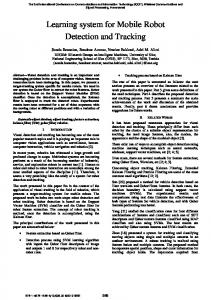
Figure 1: Hardware setup consisting of a Pioneer P3-AT outdoor robot, camera/mirror assembly for panoramic vision, a laptop and a joystick for manual route teaching.
The mobile platform used is the Pioneer P3-AT outdoor robot shown in Figure 1. A webcam directed towards a panoramic mirror provides panoramic views with a vertical Field Of View (FOV) ranging from −90◦ to 48◦ in elevation and 360◦ in azimuth. The mirror has the profile given in [Chahl and Srinivasan, 2000]. A sky shade improves the camera automatic gain control. It is wrapped in aluminium foil so its brightness follows the ambient lighting. A lens hood was used to mitigate the problem of lens flares. The camera/mirror assembly is 130cm above the ground.
3 3.1
Appearance Based Route Following System Overview
The core concept is to capture a sequence of reference panoramic images during route teaching. During the route following phase, the measurement image is compared against the closest reference image to recover a relative orientation. Only the frontal 180 degrees field of view is used to ensure a convergent behaviour. The robot then corrects its heading to zero the relative orientation. Both lateral offset and orientation error can be corrected with this behaviour. Relative orientation is recovered by first unwarping the image into azimuth-elevation coordinates, followed by a cross-correlation in the azimuth axis and detecting for peaks in the correlation coefficients.
Figure 2: Autonomous route following system overview
3.2
Image Pre-processing
Identical image pre-processing steps are applied to both reference and measurement images. Input colour image is first converted into greyscale then “unwarped” (i.e. remapped) onto azimuth-elevation coordinates. An example of the original colour image and its unwarped greyscale image is shown in Figures 3(a) and 3(b) respectively, where horizontal axis is azimuth and vertical axis is elevation. Patch normalisation is then applied which transforms pixel values as follows: I 0 (x, y) = (I(x, y) − µ(x, y)) /σ(x, y)
(1)
where I(x, y) is the original and I 0 (x, y) the normalised pixel, µ(x, y) and σ(x, y) are the mean and standard
(a)
(a) Original image
(b)
(b) Unwarped greyscale image −40
−30
−20
−10
0
10
20
30
40
(c)
(c) Patched normalised
Figure 3: (a) Original colour image. (b) Converted to greyscale and mapped into azimuth-elevation coordinates, where the azimuth-axis is horizontal. (c) Patch normalised to remove lighting variations, using a neighbourhood of 17 by 17 pixels.
Figure 4: (a) Reference image. (b) Measurement image during route following. (c) Image cross-correlation coefficients. are calculated offline and stored after route teaching. Figure 4 shows a typical ICC result between a pair of reference and a measurement images.
3.4 deviation of pixel values in a neighbourhood centred around I(x, y). A neighbourhood size of 17 by 17 pixels has worked well in the experiments. The image in Figure 3(b) after patch normalisation is shown in Figure 3(c).
3.3
Image Cross Correlation
This section addresses the problem of measuring an orientation difference between the measurement image and the reference image. Ground surface along the route is assumed to be locally flat such that the radial axis of the panoramic vision system is perpendicular to the ground plane. Orientation difference between reference and measurement image is therefore only a shift along the azimuth axis. This shift is recovered using Image Cross-Correlation (ICC) performed efficiently in the Fourier domain: φ −1 NX λ = F −1 F{Ri } · F {M i } (2) i=0
where λ is the ICC coefficients, Ri and M i are the i’th row in the reference and measurement image respectively, Nφ is the height of the image (i.e. the number of divisions in elevation), and F{•} is the Fourier transform operator. Fourier transform of the reference images
Along Route Localisation
A Markov localisation filter [Fox et al., 1999] tracks the robot’s position along the route, where the state variable is the distance from the starting point. States are discretised at a uniform resolution of 7cm per state. Distance between reference images are larger and also at a variable resolution. Selecting reference images is non-trivial. They should be allocated densely at turns or when visual features are close to the robot. This paper employs a simple selection method where reference images are allocated with a maximum separation of 35cm and 5◦ rotation according to odometry. More sophisticated reference image selection methods will be investigated in the future. There is no need for global localisation since the “kidnapped robot problem” is not one of the operation scenarios and that the robot is always initialised at the starting point. Thus at any instant in time, only a local neighbourhood of localisation states centred at the most likely robot location is considered to reduce computational complexity. Filter prediction update involves shifting the probability distribution along the route according to odometry measurement. During observation update, observation likelihood is calculated from ICC coefficients. ICC is performed on the measurement image against 11 reference images centred around the current robot location. Local maxima in the ICC coefficients are detected. For each
reference image, the score of a single local maxima with an relative orientation value closest to that of the current estimated robot relative orientation determines the matching likelihood of that reference image. The robot’s relative orientation and its estimation is discussed in the next section. Because the localisation states are denser than the reference images, each state is then given a score via linear interpolation of scores of the reference images in front and behind that state. The actual observation likelihood is obtained by first normalising the scores, followed by addition of a constant, and renormalisation. A larger additive constant has the effect of reducing the confidence placed in the observations. This constant was experimentally determined. More details are available in [Zhang and Kleeman, 2007].
3.5
4
Relative Orientation Tracking
The robot’s “relative orientation” is denoted by θδ and it refers to the difference between the robot’s current orientation and that of the reference image. A Kalman filter tracks this quantity. Prediction and correction updates are presented next. Prediction update uses readings from odometry as follows: θδ (d + ∆d) = θδ (d) + ∆θmsur (d + ∆d) − ∆θref (d + ∆d) (3) where d is the distance from the start of the route, ∆d is the distance traveled since the last update, ∆θmsur (d + ∆d) and ∆θref (d + ∆d) are the changes in orientation measured by odometry in the distance interval [d, d+∆d] during the autonomous and teaching runs respectively. Observation update uses ICC results from only two reference images. One is immediately in front and the other behind the current estimate of the robot location. One local maxima from each reference that are nearest to the current predicted θδ are selected. A linear interpolation of the two maxima positions provide the observation of θδ . The observation needs to pass a validation gate set at 95% confidence before being accepted for state update.
3.6
Robot Control
The control algorithm aims to zero the relative orientation using a proportional controller: ω = −κ · θδ
Figure 5: From top: Reference image, measurement image, result of frame differencing
(4)
where ω is the robot’s rate of rotation and κ is the experimentally determined system gain that depends on the system’s processing speed and the robot dynamics. Translational velocity is set at 25cm/s in straight sections and 15cm/s in tight turns.
Image Comparison Algorithms
The measurement image aquired while the robot is patrolling is compared against the reference image to check for anomalous entities not present during the training run. The easiest way to find these anomalies would be to subtract the measurement image from the reference image. However, even a minor deviation in the position along the path leads to misalignment in the camera images, resulting in a large amount of noise in the differenced image, as shown in Figure 5. The problem can be recast as one of finding stereo correspondences between the measurement image and the reference image. Any anomalies will appear as regions in the measurement that have no correspondence in the reference. The following sections present two representative approaches to stereo correspondence and we adapt them for anomaly detection. Section 4.1 uses sparse stereo and Section 4.2 uses dense stereo.
4.1
Sparse Stereo Based Anomaly Detection
This algorithm finds sparse feature correspondences between images. A pyramidal implementation of the iterative Lucas-Kanade feature tracker [Bouguet, 2000] from the OpenCV library [Intel, 2000] is used to find corresponding points in the measurement image to points on a grid in the reference image. Anomalous regions generate spurious or badly matched correspondences. Feature correspondence for a grid of points in the reference image is shown in the third image of Figure 6 and the points with correspondences larger than an empirically determined threshold distance are shown in the fourth image. It can be seen that these points are roughly scattered on the person, which is the anomalous entity. These points are dilated and binarised to create a mask image (image five in Figure 6) with which to filter the difference image. The filtered difference image is shown as the sixth image.
4.2
Dense Stereo Based Anomaly Detection
This section uses a dense stereo algorithm for anomaly detection. The epipolar lines for a pair of spherically projected images are curves. Because the relative offset of the robot position at the measurement image from that of the reference image is not known, the location of the epipoles are unknown as well. Hence it is necessary to assume that the epipolar lines are approximately horizontal. Some high quality anomaly detection results presented later in the paper shows that this is a reasonable assmption. A very large body of work exists for dense stereo correspondence. A comprehensive comparison of various algorithms is presented in [Scharstein and Szeliski, 2002]. Stereo correspondence using dynamic programming (DP) is an active area of research and many recent results demonstrate high quality disparity maps while maintaining real-time performance [Gong and Yang, 2007; Kim et al., 2005; Wang et al., 2006]. This section uses a simple perscanline DP algorithm described in [Scharstein and Szeliski, 2002]. There is no inter-scanline consistency enforcement. The resulting disparity map represents pixel correspondences between the reference and measurement images. Pixel pairs having a Manhattan distance in RGB greater than a threshold are considered anomalous. Occlusion regions in the disparity map are ignored. Because the epipolar lines are assumed to be horizontal but are in fact curved, there will be noise in the anomaly map. Morphological opening is applied to the anomaly map to remove small anomalous regions caused by noise. Figure 7 shows an example of DP based anomaly detection.
5
Anomaly Tracking using Particle Filtering
The particle filter uses a set of N = 1000 probabilityweighted particles (particle state is [x, y] in image coordinates) to keep track of the pdf of the anomaly position in the image over time. On start-up, particles drawn from a uniform distribution are scattered throughout the image. For each incoming image, the particles are updated, resampled and diffused. The anomaly image (output from either anomaly detection algorithm) is used to update particle weights. Each particle weight is evaluated based on the number of “on” pixels of the anomaly image in a 25-by-25 window around the particle position. Roulette-wheel selection is used to resample 96% of the particles; particles with larger pdf having greater chance of reselection. The remaining 4% of the particles are redistributed randomly throughout state space. Random redistribution prevents particles from converging on an inferior solution. Particles are perturbed from their positions by a noise fac-
Figure 6: From top: Reference image, measurement image, sparse optic flow showing magnitude and direction of flow, thresholded optic flow points, mask image, filtered difference image tor drawn from a normal distribution centred on current particle position. Over time, the particles cluster around the position of the person being tracked (Figure 8). The location of the best estimate is found as the mean particle position in a 25-by-25 window centred around the particle with highest probability. Note that the proportion of particles being resampled through the Roulette wheel technique to the proportion being redistributed ramdomly is selected empirically.
6
Experiments
Experiments were conducted in three different environments: a cluttered robotics laboratory, a corridor and an office with rows of study carrels. In each environment, the robot stored reference images at 7 cm intervals as it was manually driven through it. There were no other people around the robot except for the human operator during this training run. Note that the person remained behind the robot at all times and only appeared in a small range of angles in the panoramic images. This small strip of image was not used in the matching process. Following this, the robot was made to repeat the
(a)
Figure 7: From top: Reference image, measurement image, anomalous regions, anomalous regions after morphological opening.
(b)
(c)
Figure 8: The particles (red) cluster around the tracked person
Figure 9: From top: Reference image, result of sparse stereo, result of dense stereo. (a) A laboratory environment. (b) A corridor environment . (c) An office environment.
robotics laboratory, corridor and office environments respectively. The yellow spot is the mean particle position in a 25-by-25 window centred around the particle with highest probability.
7
Figure 10: False positives and false negatives across algorithms and experiments training route autonomously. Images captured during the autonomous runs were matched to the images in the reference set and the closest matching pairs were stored in memory. These pairs of images, one from the training run and one from the autonomous run, were then stored in sequence and compared offline. Anomalies in the images from the autonomous runs with respect to the training images were identified using the two algorithms in Sections 4.1 and 4.2. These anomalies were subsequently tracked using the particle filter outlined in Section 5. The performance of the two algorithms was compared using manually segmented ground truth in a selection of images where anomalies were present. A total of 21 images were selected from the robotics laboratory experiment, 24 from the corridor experiment and 43 from the office experiments. A few of the selected images and anomalies detected using both algorithms are displayed in Figure 9. False positives (pixels incorrectly detected as anomalous) and false negatives (failure to detect anomalous pixels) were counted for each image, and normalized with the number of anomalous pixels in the corresponding ground truth image. These false positive and false negative values across algorithms and experiments are shown in Figure 10. It can be seen that the total number of incorrectly marked pixels are greater in all cases for the sparse stereo algorithm, except for the corridor environment. However, the dense stereo algorithm has a greater number of false positives, in both the corridor and the office, possibly because of the large areas of walls in these environments with very little texture. So it can be concluded that overall, the dense stereo algorithm has a better performance over the sparse stereo algorithm, but it also has a higher number of false alarms. The tracking results on the anomaly images obtained from dense stereo are shown in Figures 11, 12 and 13 for the
Conclusion
This paper introduces a vision-based system that enables a mobile robot to follow a pre-trained route through an environment to detect and track any anomalies. The robot follows the route by comparing panoramic images to reference images aquired during training. The same images are used to detect the presence of anomalies in the environment that were not present during training. Anomaly detection is achieved using modified sparse and dense stereo algorithms. A particle filter tracks the anomalous regions. The system has the advantage that it detects both stationary and mobile anomalies while the robot itself is in motion. Its drawback is that even though minor changes in the environment since the training run, such as lights turned on or off, do not affect path following, they do affect the anomaly detection. However, we see this system being useful on a patrol robot that does after-hours surveillance of an indoor environment like a museum or office where the appearance of the environment generally remains constant.
References [Bouguet, 2000] J. Bouguet. Pyramidal implementation of the lucas kanade feature tracker. In OpenCV documentation, 2000. [Chahl and Srinivasan, 2000] J. S. Chahl and M.V. Srinivasan. A complete panoramic vision system, incorporating imaging, ranging, and three dimensional navigation. In IEEE Workshop on Omnidirectional Vision, 2000. [Davison, 2003] Andrew J. Davison. Real-time simultaneous localisation and mapping with a single camera. In Internation Conference on Computer Vision, Nice, October 13 - 16, October 2003. [duROBO, 2007] duROBO. http://www.durobo.co.kr/Eng/technology /Ofro detect01.asp, sep 2007. [Fox et al., 1999] Dieter Fox, Wolfram Burgard, and Sebastian Thrun. Markov localization for mobile robots in dynamic environments. Journal of Artificial Intelligence Research, 11:391–427, 1999. [FrontlineRobotics, 2007] FrontlineRobotics. http://www.frontlinerobotics.com/roboticstechnology/index.htm, sep 2007. FrontlineRobotics: Autonomous Perimeter Security.
Figure 11: Best particle positions over time in the lab sequence
Figure 12: Best particle positions over time in the corridor sequence
[Gandhi and Trivedi, 2004] Tarak Gandhi and Mohan M. Trivedi. Motion analysis for event detection and tracking with a mobile omni-directional camera. In ACM Multimedia Systems Journal, Special Issue on Video Surveillance, 2004. [Gong and Yang, 2007] Minglun Gong and Yee-Hong Yang. Real-time stereo matching using orthogonal reliability-based dynamic programming. IEEE Transactions on Image Processing, 16(3):879–884, 2007. [Intel, 2000] Intel. Opencv. http://www.intel.com /technology/computing/opencv/, 2000. [Jung and Sukhatme, 2004] Boyoon Jung and Gaurav S. Sukhatme. Detecting moving objects using a single camera on a mobile robot in an outdoor environment. In International Conference on Intelligent Autonomous Systems, pages 980–987, Amsterdam, The Netherlands, Mar 2004. [Kim et al., 2005] J. C. Kim, K. M. Lee, B. T. Choi, and S. U. Lee. A dense stereo matching using twopass dynamic programming with generalized ground control points. In Conference on Computer Vision and Pattern Recognition (CVPR), pages 1075–1082, 2005. [Matsumoto et al., 1999] Yoshio Matsumoto, Kazunori Ikeda, Masayuki Inaba, and Hirochika Inoue. Visual navigation using omnidirectional view sequence. In 1999 IEEE/RSJ International Conference on Intelligent Robots and Systems, 1999. [Royer et al., 2005] E. Royer, J. Bom, M. Dhome, B. Thuilot, M. Lhuillier, and F F. Marmoiton. Outdoor autonomous navigation using monocular vision. In IEEE/RSJ International Conference on Intelligent Robots and Systems, (IROS 2005), pages 1253– 1258, 2005. [Scharstein and Szeliski, 2002] D. Scharstein and R. Szeliski. A taxonomy and evaluation of dense two-frame stereo correspondence algorithms. International Journal of Computer Vision, 47(1):7–42, May 2002. [Wang et al., 2006] Liang Wang, Miao Liao, Minglun Gong, Ruigang Yang, and David Nister. High-quality real-time stereo using adaptive cost aggregation and dynamic programming. In Third International Symposium on 3D Data Processing, Visualization, and Transmission, pages 798–805, June 2006.
Figure 13: Best particle positions over time in the office sequence
[Zhang and Kleeman, 2007] Alan M. Zhang and Lindsay Kleeman. Robust appearance based visual route following in large scale outdoor environments. In 2007 Australasian Conference on Robotics and Automation (ACRA), 2007.