IEEE Power & Energy Society General Meeting 2012 (IEEE PES GM 2012) San Diego US
Anomaly Detection of Building Systems Using Energy Demand Frequency Domain Analysis Michael Wrinch, Member, IEEE, Tarek H. M. EL-Fouly, Member, IEEE, and Steven Wong, Member, IEEE Abstract—This paper presents and demonstrates a method to quickly identify when regular periodic activities, such as a daily night setback on a thermostat, are inappropriately configured or accidentally reset. Anomalies in periodic building operations are identified by analyzing smart meter electrical demand data in the frequency domain with a weekly travelling time window instead of using time domain functions such as load factor. Initial experiments on a real site found that spectral energy signals for periodic (frequency) hours of 4, 6, 8, 12 and days 1, 3.5 and 7 to be greatly reduced when a device is not functioning appropriately. In addition, the ratio of the DC offset (0 Hz) energy with the other higher periodic energies can normalize the periodic energies to a relative index that can then be used for comparing other seasons and other buildings for periodical performance. Keywords- Energy conservation, Energy efficiency, Energy management, Power system measurements, Load management, Smart grids
R
I.
INTRODUCTION
eal time interval electric utility meters or “smart meters” are becoming increasingly prevalent. This opens up the opportunity to develop advanced diagnostics and analytics for system optimization, including transformer management, outage management, and secondary cable management [1-5]. This paper describes a method to characterize an office building’s energy management system’s performance in the frequency domain and assess its performance. This technique may be used, e.g., to determine if evening, working hours and weekend setbacks are in place or to compare its energy management program to other like buildings. Owners and/or operators of commercial buildings face an ongoing maintenance challenge of knowing how their buildings are performing. Well managed buildings undergo regular recommissioning efforts in order to ensure properly functioning systems [6], but proactively identifying when a potential issue or failure occurs before an unnecessary amount of energy is consumed can be difficult. The term “re-commissioning” is used to identify activities that attempt to reduce energy use through the identification and implementation of low-cost operational and maintenance changes in a functioning building [7, 8]. Building energy analysis techniques to help evaluate and optimize building energy use, such as modified bin method or M. Wrinch is with Hedgehog Technologies, North Vancouver, BC, Canada V7L 1L7 (email:
[email protected]) T.H.M. EL-Fouly and S. Wong are with CanmetENERGY, Natural Resources Canada, Varennes, QC, Canada J3X 1S6 (e-mails:
[email protected];
[email protected]). This work was supported by Pulse Energy Inc.; Clean Energy Fund Program; Sustainable Development Technology Canada (STDC); the Innovative Clean Energy Fund (ICE); and CanmetENERGY, Natural Resources Canada.
other system simulation techniques [9], requires significant modeling. Using existing smart meter data may alleviate this burden. Additionally, operators of larger portfolios of buildings also have the challenge of determining where to direct limited resources in a way that offers the greatest benefit for managing energy. A typical metric used for building performance is occupant comfort. Unfortunately, comfort may not necessarily be jeopardized when a building controller is not functioning properly or if the controller is not optimized to minimize energy usage. Smart meter energy analytics [10] offer the advantage of diagnosing and providing first stage alerts of energy demand trends and anomalies en masse over large portfolios that are operating outside of typical parameters. Led by this concept, building energy consultants are increasingly using time-domain energy demand data to assess how building systems are functioning [7-9, 11]; however, complex periodical functions of building operations can be visualized and understood much more clearly in the frequency domain [12], where this paper focuses. Frequency domain analysis also carries the advantage of converting large data sets down to a few distinct numbers while being able to reject non-useful spectral information or noise. Common time domain diagnostics such as load factor and peak valley calculations can be used to find a relative periodicity of an energy signature [11]; however, the specific details of what the energy content is within the periodicity are not revealed hence limiting the ability to diagnose issues further with these tools. Similarly to [12], the frequency domain analysis concept is extended in this paper for use in quickly identifying, optimizing and diagnosing building automation controller issues. The two cases presented in this paper are from actual operating commercial buildings (as opposed to simulations or lab experiments). The test cases presented are located on the west coast of British Columbia, Canada. One case is presented as a reference case and the other is where the actual experiments were run. The reference case is a university office building powered by electricity and steam (steam is used for heat) with a building automation control computer controlling lighting and heat. The main test site and the primary focus of this paper, is a health facility powered 100 percent by electricity. In this building, the HVAC system is controlled by four digital thermostats located in each section of the facility, all with battery backups. The first author of this paper personally audited the site, made the corrections and monitored the energy demand before and after the modifications were made on this facility [8].
BACKGROUND
Mining interval energy demand data from smart meters for meaningful information can be a daunting task. The sheer quantity of information can exceed the practical limitations of using simple pivot tables, graphs and search functions in spreadsheets. For example, a single energy measurement point sampled in one minute intervals will result in over 525,600 samples per year. A fifteen minute measurement interval results in over 35,040 samples per year per measurement point. In addition to the quantity of information, the data itself is not always in a pristine form. For example, there can be small data gaps that may require interpolation estimates. (Note: total energy information is never lost but demand interval uploads can be missed). Reducing days, weeks, months and years of demand data down to a few simple performance metrics is the ultimate goal for developing meaningful knowledge of the system. Energy demand analysis in the frequency domain can accomplish this if the right periodical demand energies are selected. For example, if a building automation system regularly turns the building lights on and HVAC temperature up for ten hours per day, a ten hour energy demand signature will appear when viewed in the frequency domain. Typical periodic energy demand parameters of a building are difficult to generalize but there are some trends that can be detected. A typical commercial building has a periodic energy demand pattern matching the occupants’ usage and the programming/setting of its building automation system (BAS). Most commercial facilities (excluding data centers) follow a twenty-four hour energy cycle for each day and a seven day energy cycle for a typical commercial work week (such as offices and stores). However, there are often other periodical demand energy signatures created by the occupants that are less obvious, such as regular work periods (seven to eight hours), lunch breaks (four hours from the start of the day), and seasonal vacations. The building automation system should be programmed to track the behavior of the occupants and seasons (with a phase delay) so that the building’s environment is brought to an acceptable comfort level when the occupants are present while also minimizing energy usage when they are not present. Since occupants operate on a daily cycle, it is logical to assume that a non-functional building automation computer that keeps the temperature constant day and night or has improperly programmed night and weekend temperature setback features will show a weakening of the spectral electrical demand in some normally prominent bands. If this were to be observed in the frequency domain, certain normally strong periodical demand energies will show a drop or drift towards the random noise platform when a failure occurs. A one month time series plot of a commercial building’s electrical energy demand will very clearly show weekly and daily (24 hour) periodic behavior. Take that of the reference case, Fig. 1, that shows one month of the energy demand of a building that has been recently audited, re-commissioned and is in ideal working order. The building is located on a university in Vancouver, BC, Canada and is used primarily for office work. Referencing Fig. 1, there are four groups consisting of five peaks indicating week day working hours and two very small peaks indicating weekend operating activity. However, in this time-domain approach it is difficult to see other periodic
trends in the data compared to analysis in the frequency domain as seen in Fig. 2. Electrical Demand (kW) vs. Time (1 month) Commercial Facility 400
350
300
Electrical Demand (kW)
II.
250
200
150
100
0
500
1000
1500
2000
2500
3000
Time (15 min/point)
Fig. 1: One Month of Office Building's Electrical Demand (kW)
The frequency domain conversion (Fig. 2) was attained using Fourier Transformation with square windowing for one month with the result further processed by taking the square root of the squared sum of real and imaginary values. The amplitude (y-axis) is scaled to the actual power. The frequency axis (x-axis) is scaled by time (in hours/cycle) of the periodic cycles instead of the usual cycles/second (Hz) that is typically characteristic of the frequency representation. This scaling is to allow the clear viewing of daily periodic schedules and periodic behavior of the building automation and occupants in terms of hours that are easy to understand. Here, high energy periodical points can be seen on the four, six, eight, twelve and twenty-four hour cycle periods (Fig. 2) indicating that throughout the month, there are not only the obvious twentyfour hour cycles but other more subtle ones present created by both computer control and occupant activities such as taking lunch which shows up in hour four. Clearly the twenty-four hour cycles are obvious from Fig. 1 but the others seen in Fig. 2 frequency domain are not. The process by which to use Fourier transform on time-series energy data is described next. III.
THEORETICAL CONCEPT
To convert a time based sampled signal to the frequency domain, the discrete Fourier transform is commonly used [13, 14]. The transform is accomplished by calculating the sum of all the products of a function at point “n” with the cosine and sine wave at point “n” in reference to a specific frequency. All frequencies are set between 0 to 2π where 2π is equal to the sampling frequency. The results for each frequency are real and imaginary values (1). The square root of the squared sum of the real and imaginary values yields the magnitude of the specific frequencies. However, whereas (1) is for continuous infinite signals, this work requires sampling of discrete time measurements. A sampled signal windowed at a finite interval contains undesirable high frequency artifacts at its sharp discontinuous
ends. This phenomenon is called the Gibbs Effect. To reduce the Gibbs Effect, a windowing function can be multiplied onto the signal such as Hamming and Hanning type windows [14]. Electrical Demand (kW) vs. Frequency (1 month window) Commercial Facility 160
Electrical Demand (kW)
140 120
( )
Take, for example, using the fifteen minute interval meters with a time window of thirty days. The formula for conversion to frequency per point would make tsample window = 30x24x60/15=2880 hours, and t(x)sample step = (60*xsample number)/15=4x where x is each time step.
( )
12hr
80
6hr 8hr
60
4hr
40 20 0
5
10 15 20 Frequency (hours/cycle)
25
30
Fig. 2: Office Building's Electrical Demand (kW) vs. Frequency
(
)
∑
[ ]
These windows slowly taper a signal’s amplitude at each end to zero, thereby diminishing the end of each window’s discontinuity causing a significant reduction in the Gibbs Effect. The windowing addition to a discretized finite length sample can be seen in (2). Since windowing creates losses in the signal and prevents the ability of summing the power at each periodical demand energy, months and weeks were aligned as accurately as possible within a square window so as to minimize discontinuities.
( )
100
0
(
)
∑
[ ]
[ ]
The fast Fourier transform (FFT) is often referenced when completing a discrete Fourier transform. The FFT is an efficient algorithm used to compute the discrete Fourier transform, but there is no loss of data in the conversion. The FFT was used for data processing of (2) in this work. The resolution of the periodical demand energy components is limited by the Nyquist frequency and the sample window. The Nyquist frequency (frequency is the inverse of the sample time, fnyquist=1/(2Tsample)) is half the sampling frequency of the signal. Undesirable aliasing or frequency folding can be avoided by only analyzing frequencies lower than or equal to the Nyquist frequency. In the case of fifteen minute sample time demand meters, the Nyquist frequency is 1/(thirty minutes). The sample window size (i.e. 1 day of samples, 1 month, 1 year, etc.) determines the frequency change per step. The frequency step of each point of the Fourier transform is then equal to the ratio of the sample window time and the time of each sample step (3). To convert fifteen minute intervals to frequency steps in hours, (3) must be converted to hours.
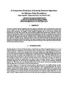
A. Normalization for Comparison When using this theory to compare different seasons or two different buildings of interest, the data must be normalized and the periodical demand energies to be used determined. Using the reference case presented as a guide, the periodical demand energies for 2, 4, 6, 8, 12 and 24 hours are all selected as points of interest for evaluation. To normalize the data for relative comparison to other seasons and similar facilities, the intensity of the periodical demand energies can be normalized in two ways: 1) By dividing the zero frequency periodical demand energy (or DC offset) by each 24, 12, 8, 6, 4, and 2 hour periodical demand energy or 2) By comparing workweek setback by weekend setback. The one day periodical demand energy can be divided by the seven day periodical demand period. If this number is close to one there may be an issue with weekend setbacks and should be further investigated. With a health facility, this may not be the case as the facility operates seven days per week. The process for the analytical experiment is illustrated in Fig. 3. The normalized periodical demand energy components, fn, are calculated as in (5), where n represents hours of the 1/( frequency) time.
[
]
[∑
[ ( )] (
]
)
The normalized periodical demand energy vectors in (5) are the points used for assessing the state of the building BAS. When the periodical demand energies experience a significant and permanent change, it may signal an issue that may be worth looking into by the building owner. The main test site, a commercial health facility located on the west coast of British Columbia, Canada that depends on electricity for all of its energy needs, was used to demonstrate the frequency domain assisted evaluation of BAS. It was chosen because all modifications made to the building were witnessed and all changes could be accounted for, making for a compelling opportunity to demonstrate the concept. Since it is a health facility, it is typically used on both weekdays and weekends with hours of operation of nine to five (seven days a week). The BAS computers are programmed considering this. The facility has no air conditioning load. Heating is controlled by four individual thermostats linked to the HVAC system and digital controls for some other line voltage baseboard heaters located at the doors. The facility was installed with a smart meter as part of a community effort to improve efficiency and explore demand side management options. The health centre’s
energy profile was monitored and recorded for one year before any changes were made. This facility was only a few years old and was originally assumed to be operating as designed, that is, efficiently, making it a low priority in a demand side management program within the community. However, this was discovered not to be the case, making its one year of collected energy data good for analysis.
Smart Meter Data Storage E(t)
Select and use Travelling Fourier Transform window
Select and normalize Harmonics with F(0) Slide Window One Step
Compare Harmonics to Baseline
NO
Outside Baseline?
and month long time windows. High intensity values from (5) , i.e. when the periodic energy (denominator) is very small and the DC is very high (numerator), indicate a problem. The change in the time domain series is very clear when viewing the demand data one month before the modification was made (Fig. 4, top graph) and the one month after the modification was made (Fig. 4, bottom graph). However, the most significant changes come from the normalized frequency series, which show substantial differences in periodical demand energy intensities, before and after the modifications were made. Before the modifications, Fig. 5, top, there are no periodical demand energies close to 5 kW except for the twenty four hour cycle, but after the modification, Fig. 5, bottom graph), significant periodical demand energies do appear (indicating that the BAS is working). By tabularizing and normalizing the periodical demand energy results before and after the BAS corrections and comparing them, one can observe that the change in periodical demand energy content is significant (Table 1). The periodical demand energy ratios (before and after the modifications) range from 4.60 to 21.64; the hour two periodical demand energy has the greatest change in ratio. The effect of the modification to the BAS (which occurred on the fifth month) can be seen by plotting the periodical demand energies vs. the month of the experiment, Fig. 6 (logarithmic plot). Each bar represents a monthly time window; the drop between bars 5 and 6 reflects when the change happened and its significance.
YES Time (one month) Vs. Power (kW) of Before Modification
Flag Time and Harmonic for reporting
IV.
EXPERIMENTAL RESULTS
Electrical energy demand data was collected in one minute and fifteen minute average demand intervals, then analyzed using the proposed algorithm for a period of five months before the modification and several months afterwards, using week
Power (kW)
30 20 10
0
4 60
Power (kW) Power (kW)
At the end of April of 2011, an energy audit was conducted on the main test site (health facility). The occupants were interviewed so as to get an initial check on the comfort level. Some occupants indicated the building was sometimes overly warm or cool, which they alleviated by opening or closing windows during the day. Further inspection into the warm and cool comments revealed that the computerized thermostats for the HVAC had lost their programs and were functioning in a nearly constant “on” state with little to no evening setbacks. The computerized thermostats were replaced the same month with newer upgrades and reprogrammed so as to meet the occupant’s comfort including a lunch time setback as everyone tended to leave the building for lunch. Baseboard heaters had similar digital thermostats, installed by an electrician on the same week, that were designed specifically for line voltage heaters. The data collected which formed the ‘baseline’ data for the analysis in this paper goes back five months; postinstallation, six months of data had been collected (up to the writing of this paper).
40
500
1000 1500 2000 2500 Time Points (one month total) Frequency (hr) Vs. Power (kW) of Before Modification Time (one month) Vs. Power (kW) of After Modification
3000
5 500
30 3000
3
40 2 201 0 00 0
10 15 20 25 1000 Frequency 1500(hours) 2000 2500 Time Points (one month total) Frequency (hr) Vs. Power (kW) of After Modification
4
Fig. 4: One Month of the Health Facility’s Demand Before (Top) and After 3 Modification, in Time Domain (Bottom) Power (kW)
Fig. 3: Analysis Process for Fourier Travelling WindowTest Case Description
50
2 1 0
0
5
10
15 Frequency (hours)
20
25
30
Power (
30 20 10
0
500
1000 1500 2000 2500 Time Points (one month total) Frequency (hr) Vs. Time (one month) Vs.Power Power(kW) (kW)ofofBefore After Modification Modification
Power Power (kW)
60 15
3000
This same experiment can be repeated by using weekly windows for the Fourier transform instead of monthly, with similar results. Weekly time windowing carries the advantage of permitting quicker fault detection.
40 10 205 00 00
5 500
10 15 20 25 1000 1500 2000 2500 Frequency Time Points (one (hours) month total) Frequency (hr) Vs. Power (kW) of After Modification
30 3000
Power (kW)
15 10 5 0
0
5
10
15 20 Frequency (hours)
25
30
It can be seen that when comparing this case with the reference ideal case shown in Fig. 2, the periodic energy signatures are all below a normalized intensity of 150 and the two and four hour energies are not present (Fig. 7, Logarithmic plot). The lack of two and four hour energies may indicate that there is no lunch-time setback for this building as there was for the case study. The intensity value of 150 indicates the reference case’s periodical functions are significant and present, however a portfolio manager would need to baseline their own buildings to match the facility’s utilization. For a failed building automation system as seen in the main test site (health facility) the intensity ratio increases logarithmically as the periodic functions tend to zero energy. 10
3
Bar Chart of Harmonic Ratios for 12 Months Reference
Table 1: Changes in Health Facility BEM System Reflected by Normalized Intensity Normalized Intensity (from F(0)) Periodical demand energy
Before (month 5)
After (month 7)
Change (Before/After)
24
23
5
4.60
12
33
7
4.71
8
54
10
5.40
6
154
21
7.33
4
289
53
5.45
2
909
42
21.64
10
Intensity (no unit)
10
10
10
10
4
Bar Chart of Harmonic Ratios for 12 Months Reference
3
2
1
0
24 Hour
12 Hour
8 Hour 6 Hour Harmonics (hours)
4 Hour
2 Hour
Fig. 6: Periodical demand energy Ratio vs. Time (Month/bar) of Health Facility
Intensity (no unit)
Fig. 5: One Month of the Health Facility’s Demand Before (Top) and After (Bottom) Modification, in Frequency Domain
10
10
10
2
1
0
24 Hour
12 Hour
8 Hour 6 Hour Harmonics (hours)
4 Hour
2 Hour
Fig. 7: Periodical demand energy Ratio vs. Time (Month/bar) for Office Building
V.
DISCUSSION OF RESULTS AND CONCLUSION
Periodical demand energy analysis of building automation system (BAS) functions simplifies large amounts of demand data into a few readable indicators (numbers), easing the job of a facilities manager and increasing their likelihood of detecting anomalies by simply observing a trend of increasing periodical demand energy ratios from the original baseline. By normalizing the values to the zero frequency point, the energy use patterns of different buildings at different times of the year and at different demand intensities can be compared with each other. This allows for evaluation against standard acceptable periodical demand energy intensity ratios. Low periodical demand energy intensity ratios in a band indicates that it has strong periodical demand energy and that computer control is operating as intended, while high periodical demand energy ratios indicate a lack of any periodical demand energy in that particular band, which may indicate a non-functional computer control system. No values for periodical demand energy bands indicate an extremely low or no periodical demand energy in that particular band. Further analysis using the power spectral
density functions may further resolve the work though this was outside of the scope of this initial evaluation. The initial stages of this research point towards focusing on periodical demand energies relating to common working hours, but there are likely other key periodical demand energies that will arise out of a comprehensive analysis of building demand data and patterns of periodical demand energies. The largest challenge with this research is gaining access to detailed demand data and linking the specific results with changes in the building’s operations. The authors were fortunate enough to have extensive access to the case presented in this paper. Though it was not shown directly in this work, 3.5 day and 7 day energy periodical demand energies tended to show periodic energy periodical demand energies with the base case, though it was inconclusive as to what the 3.5 day period periodical demand energy meant (while weekly periodic energy clearly represented a weekly cyclic energy usage.) In future work, the authors will be investigating weekly energy patterns, analyzing drift around a typical eight hour working day and conducting a more comprehensive building analysis study.
[6]
[7]
[8] [9] [10] [11] [12]
[13] [14]
(2005). Recommissioning – Optimising Building Operations (1 ed.) [HTML/PDF]. Available: http://oee.nrcan.gc.ca/publications/infosource/pub/ici/eii/m143-3-12005-e.cfm?attr=20 B. Hydro. (2010). Continuous Optimization for Commercial Buildings. Available: http://www.bchydro.com/powersmart/commercial/power_smart_partners /continuous_optimization.html B. L. Capehart, W. C. Turner, and W. J. Kennedy, Guide to energy management, 5th ed. Lilburn, GA: Fairmont Press, 2008. A.-H. Mohammad Saad, "Computer-aided building energy analysis techniques," Building and Environment, vol. 36, pp. 421-433, 2001. W. H. E. Liu, "Analytics and information integration for smart grid applications," in Power and Energy Society General Meeting, 2010 IEEE, 2010, pp. 1-3. A. Thumann and D. P. Mehta, Handbook of energy engineering, 5th ed. Lilburn, Ga.: Fairmont Press, 2001. C. Yu and D. Nan, "Research on spectral analysis method of load characteristics in smart grid," in Fuzzy Systems and Knowledge Discovery (FSKD), 2011 Eighth International Conference on, 2011, pp. 2561-2565. A. V. Oppenheim, R. W. Schafer, and J. R. Buck, Discrete-time signal processing, 2nd ed. Upper Saddle River, N.J.: Prentice Hall, 1999. A. V. Oppenheim, A. S. Willsky, and S. H. Nawab, Signals & systems, 2nd ed. Upper Saddle River, N.J.: Prentice Hall, 1997.
ACKNOWLEDGMENT This research would not have been possible without the support from Pulse Energy Inc., CanmetENERGY, Government of Canada, through the Program on Energy Research and Development; and the Gitga'at Nation from the Village of Hartley Bay. We would like to particularly thank David Benton, the Manager of Special Projects from Hartley Bay, for his continual dedication and vision towards clean energy program at Hartley Bay and Bruce Cullen, the Remote Communities Manager from Pulse Energy, for his leadership that maintains the momentum of the program. REFERENCES [1] [2] [3] [4]
[5]
F. Kupzog, T. Zia, and A. A. Zaidi, "Automatic electric load identification in self-configuring microgrids," in AFRICON, 2009. AFRICON '09., 2009, pp. 1-5. G. Pritchard, "Reading Deeper," Power and Energy Magazine, IEEE, vol. 8, pp. 85-87, 2010. A. Rautiainen, S. Repo, and P. Jarventausta, "Using frequency dependent electric space heating loads to manage frequency disturbances in power systems," in PowerTech, 2009 IEEE Bucharest, 2009, pp. 1-6. S. V. Verdu, M. O. Garcia, C. Senabre, A. G. Marin, and F. J. G. Franco, "Classification, Filtering, and Identification of Electrical Customer Load Patterns Through the Use of Self-Organizing Maps," Power Systems, IEEE Transactions on, vol. 21, pp. 1672-1682, 2006. T. Wu, W. Song, and Y. Zhang, "A new frequency domain method for the harmonic analysis of power systems with arc furnace," in Advances in Power System Control, Operation and Management, 1997. APSCOM97. Fourth International Conference on (Conf. Publ. No. 450), 1997, pp. 552-555 vol.2.
BIOGRAPHIES Michael C Wrinch (M’01) Received his B.A.Sc. degree in 2000 and M.A.Sc. degree from Memorial University of Newfoundland, Canada and his PhD from the University of British Columbia where he specialized in power system island detection. His research interests lie in emerging energy systems integration and real time demand data intelligence. He is an active member of the IEEE and he is a Professional Engineer in the province of British Columbia, Canada. Michael is currently a retained Consultant for Pulse Energy Inc. and owns Hedgehog Technologies Inc., an engineering consultancy company. Steven Wong (S'05-M'10) is a T&D Research Engineer with the Grid Integration of Renewable and Distributed Energy Resources Group at CanmetENERGY, Natural Resources Canada. He obtained a PhD in Electrical Engineering from the University of Waterloo, Canada, in 2009. His research background and interests lie in power system planning, including distributed generation, distribution and transmission systems, sustainable energy resources and storage, and innovative energy markets. He is currently working in the areas of smart grid development and photovoltaic system integration. Tarek H. M. El-Fouly (S'97-M'07) received the B.Sc. and M.Sc. degrees in electrical engineering from Ain Shams University, Cairo, Egypt, in 1996 and 2002, respectively. He received the Ph.D. degree in electrical engineering from the University of Waterloo, Waterloo, ON, Canada, in 2008. He joined CanmetENERGY, Natural Resources Canada, in 2008, as a Transmission and Distribution Research Engineer where he is conducting and managing research activities related to active distribution networks, microgrids, and remote communities. In 2010, he was appointed as Adjunct Assistant Professor at the Electrical and Computer Engineering Department at the University of Waterloo. His research interests include protection and coordination studies, integration of renewable energy resources, smart microgrid, smart remote community applications, and demand side management and forecasting.