the help system and pdf manuals included with the R distribution, the reader can find additional ... a text window for the entry of commands and display of textual output (Fig. ..... length one or more, giving maximal dimensions in each of the directions. ...... A1.10 Custom axes created and annotated using the function axis.
Appendix A R Syntax in a Nutshell
Here we give an overview of the syntax and basic usage of the R language. We describe how to start and stop an R session, obtain help and find documentation. An account of the main object types and their manipulation in direct (i.e. command line) mode is followed by text on arguably the strongest point—graphics. The Appendix is closed by a section on writing true R programs (batch mode). The text is partly based on the pdf file ‘An Introduction to R’, available from the Help menu. This text does not intend to be a replacement for a proper R course. Apart from the help system and pdf manuals included with the R distribution, the reader can find additional information in an increasing number of books and web sites. Importantly, information concerning the current state of the R project, binaries, source codes and documentation are obtainable from the dedicated website (www.r-project.org) and the Comprehensive R Archive Network (CRAN, cran.rproject.org). CRAN, which is mirrored at many servers worldwide, also provides a distribution channel for user-contributed packages that add new functionality to the core of the R system.
Chapter 1 Direct Mode 1.1
Basic Operations
1.1.1 Starting and Terminating the R Session In Windows, double clicking the file RGUI.EXE or the associated shortcut opens the“R Console”, a text window for the entry of commands and display of textual output (Fig. A1.1). The system prints a number of messages, the most important of which is the last line with a prompt, showing that the R environment is awaiting commands. Apart from the R Console, one or more windows for graphical output and help pages may be displayed. © Springer-Verlag Berlin Heidelberg 2016 V. Janoušek et al., Geochemical Modelling of Igneous Processes – Principles And Recipes in R Language, Springer Geochemistry, DOI 10.1007/978-3-662-46792-3
277
278
Appendix A R Syntax in a Nutshell
To end an R session, one can invoke the menu item File|Exit or type q(). Alternatively, one can terminate the session by closing the R Console window.1
Fig. A1.1 Screenshot of a typical R session.
1.1.2 Seeking Help and Documentation The R environment provides help in several forms—including plain text (displayed in the Console) or HTML (viewed using a web browser). > help(plot) # text help on a function called ‘plot’ > ?plot
# equivalent, a shortcut
Commands related to ‘plot’: > apropos(plot)
Examples of correct usage of ‘plot’: > example(plot)
An HTML browsable help window can be obtained from the menu option Help|R language (html) or by: > help.start()
1Note
that the system may ask you, upon closing, whether you want to save the current workspace (i.e., memory image with all the variables). For beginners probably the best option is ‘No’, ensuring that the R environment starts afresh the next time.
Appendix A R Syntax in a Nutshell
279
R is distributed together with PDF documents, which can be invoked from the menu item Help|Manuals. There are several documents available, including ‘Writing R Extensions’, ‘R Data Import/Export’, ‘The R Language Definition’ and ‘R Installation and Administration’. At this stage the most appropriate will be ‘An Introduction to R’ which outlines the basics of the R language. Other good sources of information are the many books about R (e.g., Maindonald and Braun 2003; Murrell 2005; Crawley 2007; Chambers 2009; Adler 2012; van den Bogaard and Tolosana-Delgado 2013), or the related S language (Becker et al. 1988; Chambers and Hastie 1992; Chambers 1998) as the two languages share most of their syntax. CRAN contains a list of published monographs (www.r-project.org/doc/bib/R-books.html) as well as links to numerous contributed documents or manuals, both general and specific. The R Journal, an open-access refereed journal, features short to medium length articles on various R applications, R programming and add-on packages. The community meets at annual useR! conferences. Moreover, there exist e-mail discussion groups dedicated to help users (R-help), to announce new versions and further progress in the R project (R-announce, R-packages) and to facilitate communication among developers (R-devel). Further information, including the archive of the e-mail discussion groups, is available on CRAN. Lastly, there exist numerous blogs dedicated to the R project, most of them accessible from the R-bloggers web page, www.r-bloggers.com. A useful starting point to search for a topic is RSeek, www.rseek.org.
1.2
Fundamental Objects of the R Language
1.2.1 Commands The R environment can be utilized in direct mode, typing commands straight into the Console and getting an immediate response. Alternatively, the whole R code can be prepared in advance as a plain text file and run at once in batch mode. The commands (functions) in R are entered either individually, each on a single line, or are separated by a semicolon (;). More complex statements consisting of several lines of code are enclosed in braces {}. Each command is followed by brackets with parameters (or empty, if none are required or default values are desired). Typing just the command name returns a listing of the function’s definition.
The R language is case sensitive. Commands are typed in lowercase and the environment distinguishes between lower and upper case letters in variable names. The latter cannot start with a digit and may contain any symbols apart from the hash mark (“#”). Note however that it is not wise to use, for instance, accented characters. It is also important to note that several words are reserved by the system and cannot be used as variable names. For details, see ?Reserved.
280
Appendix A R Syntax in a Nutshell
Direct Mode In the simplest case, commands are entered and the result displayed: > (15+6)*3 [1] 63
The numerical values can be assigned to a named variable. Perhaps confusingly, R does not use “=” as an assignment operator. Instead, an arrow “ # My comment 2
In fact the “=” also works as an assignment operator, however it is considered to degrade the code readability. We prefer using the arrow notation throughout the book. 3 Assuming that the code resides in the current working directory; otherwise the full path needs to be specified or directory changed.
Appendix A R Syntax in a Nutshell
281
Note that in batch mode the content of a variable must be displayed using the commands print or cat (this Appendix, Chap. 3.1). Unlike in direct mode, typing the mere variable name does not suffice here. > e print(e) [1] 1.602
The usage of batch mode (and graphical capabilities) of R is best demonstrated by running some built-in demos, such as: > demo(graphics) > demo(image)
1.2.2 Handling Objects in Memory R stores data using a variety of object types including vectors, arrays, matrices (two-dimensional arrays), factors, data frames, lists and functions (Table A1.1). To display the current list of user objects, use the menu Misc|List objects or: > ls()
Unnecessary objects can be removed with the function rm: > rm(x,y,junk)
All user R objects can be deleted using the menu item Misc|Remove all objects. Table A1.1 Overview of the most important object types in the R language Can have several modes?
Object
Characteristics
Possible modes
Vector
one-dimensional collection of elements
numeric, character, complex, logical
No
Factor
each element is set to one of several discrete numeric, character values, or levels (a categorical variable)
No
Array
multidimensional collection of elements
numeric, character, complex, logical
No
Matrix
two-dimensional array
numeric, character, complex, logical
No
Data frame
like a matrix but every column can be of a different mode
numeric, character, complex, logical
Yes
List
consists of an ordered collection of objects (components) that can be of various modes (recursive, i.e. list can itself consist of lists)
numeric, character, complex, logical, function, expression, formula
Yes
Function
fundamental piece of code, typically dedicated to a single task, with defined input parameters (arguments) and output values
–
–
282
Appendix A R Syntax in a Nutshell
All the objects are stored in memory, and not automatically saved to disc. When quitting the R environment, you are given the opportunity to save the current workspace, i.e. all the objects created during the given session. If you accept, they are written to a file.RData in the current directory and reloaded automatically the next time R is started. Different R sessions may therefore be maintained in separate directories.
1.2.3 Attributes to Objects Every object possesses several properties, called attributes. The two most important of these are length and mode. Some object types, or in R jargon classes, can have more modes. For the given object, the mode (logical, numeric, complex or character) can be displayed using the namesake function: > mode(10) [1] "numeric"
1.3
Numeric Vectors
1.3.1 Assignment Assignment of several items to a vector is done using the combine function c: > x y y [1] 10.4 5.6 3.1 6.4 21.7 0.0 10.4
5.6
3.1
6.4 21.7
1.3.2 Vector Arithmetic For vectors, calculations are made using basic arithmetic operators: + - * / ^. The use of these operators for two vectors of the same length is intuitive. In other cases, the elements of the shorter vector are recycled as often as necessary. For instance, for the x vector defined above, we can calculate:
Appendix A R Syntax in a Nutshell
> x*2 [1] 20.8 11.2 > x*c(1,2) [1] 10.4 11.2
283
6.2 12.8 43.4 3.1 12.8 21.74
1.3.3 Names Each vector may have an attribute names (the lengths of the vector itself and its names must be matching!). For instance: > x names(x) x Opx Cpx Pl 3 15 27
1.3.4 Generating Regular Sequences Regular sequences with step 1 or -1 can be generated using the colon operator (“:”). It has the highest priority within an expression, higher than the other operators (+-*/^). > 1:9 [1] 1 2 3 4 5 6 7 8 9 > 9:1 [1] 9 8 7 6 5 4 3 2 1 > 1:9*2 [1] 2 4 6 8 10 12 14 16 18 > 1:(9*2) [1] 1 2 3 4 5 6 7 8 9 10 11 12 13 14 15 16 17 18
seq(from, to, by) Yields a sequence of numbers with an arbitrary step (by): > seq(30,22,-2) [1] 30 28 26 24 22
rep(x, times) Repeats the argument x specified a number of times: > x rep(x,5) [1] 3 9 3 9 3 9 3 9 3 9
4
NB that this is not a dot (scalar) product, but simply a result of an element-wise multiplication.
284
Appendix A R Syntax in a Nutshell
1.3.5 Functions to Manipulate Numeric Vectors The R language contains a number of functions. Only those most important for manipulation of numeric vectors are presented in Table A1.2. Information about others and the whole range of available parameters can be found in the R documentation. Table A1.2 Basic functions for numeric vectors manipulation Function
Explanation
abs(x)
absolute value
sqrt(x)
square root
log(x)
natural logarithm
log10(x) log(x,base)
common (base 10) logarithm logarithm of the given base
exp(x)
exponential function
sin(x) cos(x) tan(x) min(x)
trigonometric functions minimum
max(x)
maximum
which.min(x)
index of the minimal element of a vector
which.max(x) range(x)
index of the maximal element of a vector range of elements in x; equals to c(min(x),max(x))
length(x)
number of elements (= length) of a vector
rev(x)
reverses the order of elements in a vector
sort(x)
sorts elements of a vector (ascending)
rev(sort(x)) round(x,n)
sorts elements of a vector (descending) rounds elements of a vector to n decimal places
sum(x)
sum of the elements of a vector
mean(x)
mean of the elements of a vector
prod(x)
product of the elements of a vector
1.4
Character Vectors
Character vectors are collections of text strings, i.e. sequences of characters delimited by the double quote symbol, e.g., "granite". They use \ – backslash as the escape sequence for special characters, including “\t” – tab and “\n” – new line.
Appendix A R Syntax in a Nutshell
285
paste(x, y, …, sep="") Merges two (or more) character vectors, one by one, the elements being separated by string sep: > paste("Gabbro","olivine and","pyroxene",sep=" with ") [1] "Gabbro with olivine and with pyroxene"
substring(x, start, stop) Extracts a part of vector x starting at position first and ending at last: > x substring(x,1,4) [1] "Plag" "Biot" "Musc"
strsplit(x, split) Splits the strings in x into substrings based on the presence of split. Returns a list (see this Appendix, Chapter 1.8): > x strsplit(x,"a") [[1]] [1] "Pl" "giocl" "se" [[2]] [1] "K-feldsp" "r"
1.5
Logical Vectors
Logical vectors consist of elements that can attain only two logical values: TRUE or FALSE. These can be abbreviated as T and F, respectively. In the R language, the symbol name F is reserved as an abbreviation for logical FALSE. For this reason, it is not advisable to name any variable F. The same applies, of course, to T.
1.5.1 Logical Operators The logical vectors are typically produced by comparisons using operators < (smaller than) (greater than) >= (greater or equal to) == (equals to) != (does not equal to). For instance: > x x > 13 [1] FALSE FALSE TRUE TRUE FALSE FALSE
286
Appendix A R Syntax in a Nutshell
The result can be assigned to a vector of the mode logical: > temp 13 > temp [1] FALSE FALSE
TRUE
TRUE FALSE FALSE
Boolean arithmetic combines two or more logical conditions using the logical operators: and(&), or(|), not(!)with or without brackets: > x c1 10 > c2 c2 [1] TRUE TRUE FALSE FALSE TRUE TRUE > c1 & c2 # logical "and" [1] FALSE TRUE FALSE FALSE TRUE FALSE > c1 | c2 # logical "or" [1] TRUE TRUE TRUE TRUE TRUE TRUE > !c1 # negation [1] TRUE FALSE FALSE FALSE FALSE TRUE
1.5.2 Missing Values (NA, NaN) Within R, missing data are represented by a special value NA (not available). Some operations which give no meaningful result in the circumstances will return its special form, NaN (not a number): > sqrt(-15) [1] NaN
Moreover, division by zero gives + ∞ (Inf). > 1/0 [1] Inf
is.na(x) Tests for the presence of missing values in each of the elements of the vector x: > x is.na(sqrt(x)) [1] FALSE FALSE TRUE FALSE TRUE TRUE
1.6
Arrays, Matrices, Data Frames
Several kinds of table-like objects exist in R. Data frames are data objects to be processed by statistics, with “observations” as columns (elements/oxides in geo-
Appendix A R Syntax in a Nutshell
287
chemistry) and “cases” (samples) in rows. They can contain columns of any mode, even mixed modes; thus they are not intended for matrix operations. For such purpose, matrices should be used. All elements of a matrix can only be of a single mode (numeric, most commonly). Arrays are generalized matrices: they must have a single mode but can have any number of dimensions. Although superficially similar, these three types of objects must not be confused. Depending on the exact content of the file, many file reading operations (such as read.table) would generate a data frame: it is the user’s responsibility to convert it to a matrix if it is to be used later for calculations. matrix(data = NA, nrow = 1, ncol = 1, byrow = FALSE) This command defines a matrix of nrow rows and ncol columns, filled by the data (if data has several elements, they will be used down columns, unless an extra parameter byrow=TRUE is provided). For instance: > x x [,1] [,2] [,3] [,4] [1,] 1 4 7 10 [2,] 2 5 8 11 [3,] 3 6 9 12 > x x [,1] [,2] [,3] [,4] [1,] 1 2 3 4 [2,] 5 6 7 8 [3,] 9 10 11 12
The default behaviour for filling a matrix with data—as well as matrix division by a vector—proceeds along columns, not rows! array(data = NA, dim = length(data)) Defines a new data array and fills it with data. The argument dim is a vector of length one or more, giving maximal dimensions in each of the directions.
1.6.1 Matrix/Data Frame Operations Matrices can be subject to scalar operations using the common operators ( +-*/^). Similar to vectors, the shorter component is recycled as appropriate. Useful functions for matrix/data frame manipulations are summarized in Table A1.3.
288
Appendix A R Syntax in a Nutshell
Table A1.3 Basic matrix/dataframe-related functions Function
Explanation
nrow(x)
number of rows
ncol(x)
number of columns
rownames(x)
row names
colnames(x)
column names binds two objects (matrices or data frames) of the same ncol (or vectors of the same length) as rows binds two objects (matrices or data frames) of the same nrow (or vectors of the same length) as columns
rbind(x,y) cbind(x,y) t(x) apply(X,MARGIN,FUN)
transposition applies function FUN (for vector manipulations) along the rows (MARGIN = 1) or columns (MARGIN = 2) of a data matrix X
x%*%y
matrix multiplication (does not work on data frame!)
solve(A)
matrix inversion (see Appendix C)
dix(x)
diagonal elements of a matrix
It is worth noting that matrix multiplication is performed using the %*% operator. Of the functions presented in the table, some explanation is required for apply: apply(X, MARGIN, FUN, …) If X is a matrix, it is split into vectors along rows (if MARGIN = 1) or columns (if MARGIN = 2). To each of these vectors is applied the function FUN with optional parameters ... passed to it. For instance, we can calculate row sums of a matrix: > x apply(x,1,sum) [1] 10 26 42
1.7
Indexing/Subsetting of Vectors, Arrays and Data Frames
In real life, one often needs to select some elements of a vector or a matrix, fulfilling certain criteria. This data selection functionality can be achieved using logical conditions or logical variables placed in square brackets after the defined object name. Subsets can be also used on the left hand side of the assignments when replacement of selected elements by certain values is desired.
Appendix A R Syntax in a Nutshell
289
1.7.1 Vectors Subsets of a vector may be selected by appending to the name of the vector an index vector in square brackets. For example, first create a named vector: > x names(x) x Pl Bt Mu Q Kfs Ky Ol Px C 1 12 15 NA 16 13 0 NA NA
Index vectors can be of several types: logical, numeric (with positive or negative values), and character: 1.
Logical vector
> x[x>10] # all elements of x higher than 10 (or NA) Bt Mu Kfs Ky 12 15 NA 16 13 NA NA > x[!is.na(x)] # all elements of x that are available Pl Bt Mu Kfs Ky Ol 1 12 15 16 13 0
2.
Numeric vector with positive values
> x[1:5] # the first five elements Pl Bt Mu Q Kfs 1 12 15 NA 16 > x[c(1,5,7)] # 1st, 5th and 7th elements Pl Kfs Ol 1 16 0
3.
Numeric vector with negative values (specifies elements to be excluded)
> x[-(1:5)] # all elements except for the first five Ky Ol Px C 13 0 NA NA
4.
Character vector (referring to the element names)
> x[c("Q","Bt","Mu")] Q Bt Mu NA 12 15
1.7.2 Matrices/Data Frames Elements of a matrix are presented in the order [ row,column]. If nothing is given for a row or column, it means no restriction. For instance: > x[1,] > x[,c(1,3)] > x[1:3,-2]
# (all columns) of the first row # (all rows) of the first and third columns # all columns (apart from the 2nd) of rows 1–3
290
Appendix A R Syntax in a Nutshell
If the result is a single row or column, it is automatically converted to a vector. To prevent such a behaviour, one can supply an optional parameter drop=F, e.g.: > x[1,,drop=F]
# (all columns) of the 1st row, keep as matrix
Moreover, matrices can be manipulated using index arrays. This concept is best explained on an example. Let’s assume a matrix defined as: > x i i [,1] [,2] [1,] 1 3 [2,] 2 2 [3,] 3 1 > x[i] [1] 9 6 3 > x[i] x [,1] [,2] [,3] [,4] [,5] [1,] 1 5 0 13 17 [2,] 2 0 10 14 18 [3,] 0 7 11 15 19 [4,] 4 8 12 16 20
The situation for multidimensional arrays is analogous—just the appropriate number of dimensions is higher.
1.8
Lists
Lists are ordered collections of other objects, known as components, which do not have to be of the same mode or type. Thus lists can be viewed as very loose groupings of R objects, involving various types of vectors, data frames, arrays, functions and even other lists. Components are numbered and hence can be addressed using their sequence number given in double square brackets, x[[3]]. Moreover, components may be named and referenced using an expression of the form list_name$component_name. Subsetting is similar to that of other objects, described above. list.name < - list(component_name_1=, component_name_2=…) Builds a list with the given components.
Appendix A R Syntax in a Nutshell
291
Here is a simple real-life example of a list definition: > x1 x2 x3 names(x3) luckovice luckovice $ID [1] "Gbl-4" $Locality [1] "Luckovice" "9 km E of Blatna" "disused quarry" $Rock [1] "melamonzonite" $major SiO2 TiO2 Al2O3 Fe2O3 FeO MgO CaO 47.31 1.05 14.94 2.23 7.01 8.46 10.33
As well as some examples of subsetting: > luckovice[[1]] [1] "Gbl-4" > luckovice$Rock # or luckovice[[3]] [1] "melamonzonite" > luckovice[[2]][3] [1] "disused quarry" > luckovice$major[c("SiO2","Al2O3")] SiO2 Al2O3 47.31 14.94
1.9
Coercion of Individual Object Types
R is generally reasonably good at dealing seamlessly with data types, converting them on the fly when needed and being able to use the same operators on different data types. When necessary, there are a series of functions for testing the mode or type of an object: is.numeric(x), is.character(x), is.logical(x), is.matrix(x), is.data.frame(x) At times there is a need to explicitly convert between data types/modes using functions such as: as.numeric(x), as.character(x), as.expression(x) Less straightforward are: as.matrix(x), as.data.frame(x) which attempt to convert an object x to a matrix or data frame, respectively. A more user-friendly way of converting data frames to matrices is provided by the function data.matrix that converts all the variables in a data frame x to numeric mode and then binds them together as the columns of a matrix.
292
1.10
Appendix A R Syntax in a Nutshell
Factors
Factors are vector objects used for discrete classification (grouping) of components in other vectors of the same length, matrices or data frames. In statistical applications, these often serve as categorical variables.
1.10.1 Basic Usage of Factors factor(x) The (unordered) factors are set by the function factor where x is a vector of data, usually containing a small number of discrete values (known as levels). In this case the levels are stored in alphabetical order. For instance: > x factor(x) [1] Pl Bt Pl Pl Kfs Pl Bt Pl Levels: Bt Kfs Pl
ordered(x, levels) This function defines a special type of factor in which the order of levels is specified explicitly using the namesake parameter. Following the previous example: > ordered(x,c("Pl","Kfs","Bt")) [1] Pl Bt Pl Pl Kfs Pl Levels: Pl < Kfs < Bt
Bt
Pl
levels(x) Returns all possible values (levels) of the factor x.
1.10.2 Conversion of Numeric Vectors to Factors In some cases it is advantageous to divide the total range of a numeric vector x into a certain number of discrete ranks (groups), and code the values in x according to the rank they fall into. If each of these ranks is labelled by identifying text, the result is a factor of the same length as the original vector. cut(x, breaks, labels) The function cut splits a numeric vector x into a number of ranks and classifies its items accordingly. The argument breaks either defines cut-off values or a desired number of intervals. Parameter labels may provide names for individual ranks. For an example of use, see Part I, Exercise 2.7.
Appendix A R Syntax in a Nutshell
293
1.10.3 Frequency Tables table(…) This function counts the number of occurrences of the given level within the factor. A pair of factors defines a two-way cross-classification (a frequencycontingency table) (Part I, Exercise 2.8).
1.10.4 Using Factors to Handle Complex Datasets Examples of using factors to deal with complex geochemical datasets are given in Part I, exercises 2.5 and 2.6, the relevant syntax is presented here. tapply(x, INDEX, FUN, …) The components of the vector x are split into several (non-empty) groups of values, based on levels of the factor INDEX (or list of two factors) of the same length. Then a function FUN is applied to each of the groups, optionally with further arguments (...) passed to it. The vector and the factor used for grouping collectively form a so-called ragged array, since the group sizes are typically variable. aggregate(x, by, FUN, …) Applies function FUN to each of the variables (columns) of a numeric matrix or data frame x respecting grouping given by factor (or list of factors) by. Each of the variables in x is split into subsets (rows) of identical combinations of the components of by, and FUN is applied to each such a subset. Again, further arguments can be passed to FUN, as desired, via the ... argument. by(data, INDICES, FUN, …) A data frame data is split by rows into data frames subset by the values of INDICES (a factor or list of factors). The function FUN is applied to each such subset (data frame) with further arguments in ... passed to it. In fact the function by is an object-oriented wrapper for tapply designed to deal with data frames.
1.11
Data Input/Output, Files
1.11.1 Reading Data The tools for data handling and editing available in R are fairly limited and thus it is a good idea to prepare them beforehand in a dedicated application, such as a spreadsheet or database program.
294
Appendix A R Syntax in a Nutshell
Several packages are available on CRAN to help communicate with databases using SQL or ODBC protocols. Moreover there is a package interfacing to Windows applications (including MS Excel) via the DCOM interface. If you require any of these sophisticated tools, see the “R Data Import/Export” pdf documentation file. In many situations it will be sufficient to import plain text files. The most powerful of the functions available for this purpose is:
read.table(filename, header = FALSE, sep = "", na.strings = "NA", check.names = TRUE, quote = "\"'", dec = ".", fill = !blank.lines.skip) This function imports a data file specified by ‘filename’, in which the individual items are separated by separator sep. The common separators are “,” – comma, “\t” – tab, and “\n” – new line. The parameter dec specifies a character interpreted as a decimal point. Note that the result is a data frame (and not a matrix), even if the file contains only numerical values. If matrix operations are to be employed, the data object must be explicitly converted. Unless the full path is specified, the file is searched for in the current working directory. The directory can be queried with the getwd() command and set with the setwd(dir) function or the menu option File|Change dir... A parameter worth resetting to FALSE is check.names as it determines whether the row and column names are to be syntactically checked to be valid R names. When TRUE, R will replace e.g. accented characters and slashes (“/”) with dots. There is a useful convention; if the first row in the data file has one item less than the following ones, it is interpreted as column names and every first item in subsequent rows as a respective row name. The file might look as follows: SiO2 ĺ TiO2 ĺ Al2O3 ĺ Fe2O3 ĺ FeO Li1 ĺ 51.73 ĺ 1.48 ĺ 16.01 ĺ 1.03 ĺ 7.06 Li2 ĺ 51.88 ĺ 1.48 ĺ 15.93 ĺ 0.99 ĺ 6.85 …
In order to read a text file in which the lengths of rows are all the same, but column names are present, one can employ header=TRUE,row.names = 1). Parameter na.strings specifies text strings to be interpreted as missing values, e.g., na.strings=c("b.d.","-","NA"). It is fairly common for a file exported from a spreadsheet such as MS Excel to have all trailing empty fields and their separators omitted. To read such files set fill = TRUE or simply copy and paste the data from a spreadsheet to your text editor directly using the Windows clipboard. readClipboard() In its simplest form, this function reads the text from the Windows clipboard.
Appendix A R Syntax in a Nutshell
295
1.11.2 Sample Data Sets R and its packages contain numerous sample datasets that can be attached to the current session using the function data(…). For instance: > data(islands)
Then documentation is available using the help command: > ?islands
1.11.3 Saving Data write.table(x, file = "", append = FALSE, sep = " ",na = "NA", dec = ".", row.names = TRUE, col.names = TRUE) This function writes an object x (a matrix, a data frame, or an object that can be converted to such) to the specified file, separating the individual items by sep. As for read.table, one can specify the strings representing the missing values and the decimal point. Moreover, there are logical parameters determining whether row and/or column names are to be stored (row.names,col.names) and whether to append the data without erasing those possibly already present. writeClipboard(str) Writes the text specified by the character vector str to the Windows clipboard.
Chapter 2 Graphics A key benefit of using R is the large range of functions for the production and export of (near) publication-quality diagrams. They can be divided into two types; high-level functions that open a new graphical window and set up a coordinate system of the brand new graph (Table A1.4) and low-level functions that annotate pre-existing plots (Table A1.5). Note also that some of the functions (e.g., curve) can show both types of behaviour depending on the given arguments.
2.1
Obtaining and Annotating Binary Plots
plot() This is a key plotting function. For two numeric vectors, it produces a binary plot [plot(x,y)]. If one vector is shorter, it is recycled as appropriate.
296
Appendix A R Syntax in a Nutshell
A quick peek at objects, classes and methods… There are special methods of plot to handle many types of R objects. A factor for instance produces a barplot of its individual levels whereas an object created by hierarchical clustering plots as a dendrogram. This is a consequence of R being an object-oriented language whereby a function can be used on any type of data (class) for which the method (e.g., plot or print) has been defined. Often it is possible to plot most objects directly, without the need to restructure the data; the appropriate x and y values are extracted as required. Developers can extend the capabilities by creating new classes and associated methods. Table A1.4 An overview of the selected high-level graphical functions in R Function
Purpose
plot(x,y)
binary plot x vs. y (two numeric vectors)
curve(expr,from,to)
curve specified by expr (written as a function of x) in the interval from–to
contour(x,y,z)
contour plot (x and y specify a regular grid, z the values)
filled.contour(x,y,z)filled contour plot (x and y specify a regular grid, z the values) boxplot(x) coplot(formula)
“box-and-whiskers” plot conditioning plot; if formula = y~x|z, bivariate plots of x vs. y for each level of the factor z
pairs(x)
matrix of all possible bivariate plots between columns of x (matrix or data frame)
hist(x)
histogram of frequencies for x
pie(x)
circular pie-chart
When calling the function plot, and indeed many other graphical functions, a number of additional parameters can be specified to modify the appearance of the plot. Some are fairly universal (e.g., col or pch), but others are restricted or may behave unexpectedly. An overview of the most commonly used graphical parameters is given in Table A1.6. If in doubt, the manual page of the particular plotting function should be consulted. Colours may be arranged into collections called palettes. The codes for available plotting symbols, standard colours and preview of palettes are in Fig. A1.2. The complete set of graphical parameters supported by many standard R functions can be obtained using ?par. For detailed explanation, and other topics related to R graphics, see the monograph of Murrell (2005).
Appendix A R Syntax in a Nutshell
297
Table A1.5 An overview of the most useful low-level graphical functions in R Function (basic use)
Explanation
points(x,y,type="p")
adds extra data points at [x,y]
text(x,y,labels)
adds text specified by labels at [x,y]
mtext(text,side)
places text at margins, outside the plotting region on side (1 = bottom, 2 = left, 3 = top, 4 = right)
contour(x,y,z,add=TRUE)
contour plot (x and y specify the regular grid, z the values)
lines(x,y,type="l") curve(expr,add=TRUE)
joins the points with straight line segments adds a curve specified by expr (a function of x)
arrows(x0,y0,x1,y1)
arrows from [x0,y0] to [x1,y1]
abline(a,b)
straight line defined by intercept (a) and slope (b)
abline(v=x),abline(h=y)
vertical or horizontal straight line(s) grid with nx cells horizontally and ny vertically
grid(nx,ny=nx)
rect(xleft,ybottom,xright,ytop)rectangle given left, bottom, right and top limits polygon(x,y)
polygons whose vertices are given in x and y
axis(side,at,labels)
custom axis; side = 1 for x, 2 for y; at = values to be annotated bylabels
box(which)
box around the plotting region (which = "plot") or "figure", "inner", "outer"
legend(x,y,legend,lty,lwd,pch) adds a legend at the point [x,y] title(main,sub,xlab,ylab)
main title/subtitle or axes labels to the plot
palette(value) This function serves to view or manipulate a colour palette. Optional parameter value is the name of palette predefined in standard R. For instance: > ee ee [1] "red" "#FF5500" "#FFAA00" "yellow"
"#FFFF80"
abline(a = NULL, b = NULL, h = NULL) This command is used to draw a straight line. For instance: > abline(a,b) > abline(h=y) > abline(v=1:5,lty="dotted")
# slope b, intercept a # horizontal line(s) # vertical dotted grid lines
298
Appendix A R Syntax in a Nutshell
Table A1.6 An overview of the main graphical parameters Parameter
Meaning
Example
adj
text justification relative to the coordinates [x,y]
0 – left, 1 – right, 0.5 – centered
asp
aspect ratio y/x
asp = 1
axes
logical, should the axes be drawn?
axes = FALSE
bg
background colour
bg = "khaki"
cex
relative character size expansion (of text cex = 2 or symbols)
cex.main,cex.sub size of plot’s title, subtitle cex.lab,cex.axis size of axes labels, tick labels col plotting colour
col = 0, col = "red"
style of axis labels
0 – parallel to the axes, 1 – horizontal 2 – perpendicular, 3 – vertical
which of the axes is/are logarithmic?
log = "xy",log = ""
lty
line type (a number or text string)
1 2 3 4
lwd
relative line width
lwd = 2
main
main title of the diagram (top)
main = "My diagram"
mar
outer margins of a plot in lines of text mar = c(4,4,0,0) c(bottom, left, top, right)
mfcol=c(nr,nc) mfrow=c(nr,nc)
splits the plotting window into nr rows mfcol = c(2,1) and nc columns, the graphs are filled by mfrow = c(2,1) columns (mfcol) or rows (mfrow)
pch
plotting character; a numeric code or a single alphanumeric symbol
pos
position of the text relative to the coordi- 1 – below, 2 – left, 3 – above, 4 – right nates [x,y]
pty
type of plot region to be used
"s" – square, "m" – maximal
srt
rotation of the text in degrees
srt = 90
sub
subtitle of the diagram (bottom)
sub = "for thesis"
type
type of the diagram
"p" – points, "l" – lines, "b" – both, "o" – overplot, "n" – none (no plotting)
xaxs, yaxs
scaling style for axes (default is extended:"r" – extended range plotted symbols cannot crash with axes) "i" – exact scaling
xlab, ylab
labels for x and y axes
xlab = "SiO2[wt.%]"
xlim, ylim
limits of the x and y axes
xlim=c(50,70)
las log
– – – –
"solid" "dashed" "dotted" "dotdash"
pch = 7, pch = "Q"
Appendix A R Syntax in a Nutshell
299
0
1
2
3
4
5
6
7
8
9
standard 6
1
11
16
cm.colors heat.colors
7
2
12
17
terrain.colors topo.colors rainbow
8
3
13
18
grays reds
9
4
14
19
blues greens cyans
5
10
15
20
violets yellows jet.colors
Fig. A1.2 Plotting symbols and colours available through the parameters pch and col (the first row, labelled ‘standard’)5 as well as some examples of palettes built-in plain R (black names) and GCDkit (brown names).
lm(formula) A function for fitting linear models. The simplest form of formula is “y~x”, i.e. y as a function of x, performing a linear regression. To see details of the resulting object use the function summary. Note that abline has a method for plotting thus generated linear fits. text(x, y, labels) This low-level function displays the given text at coordinates [x,y]. It is especially useful to label individual data points of the binary diagrams (in combination with the pos parameter). For example, using data from the calc-alkaline Sázava suite of the Variscan Central Bohemian Plutonic Complex (Janoušek et al. 2004): sazava.data
> > + > > > +
sazava ee ee Call: lm(formula = sazava[, "Ba"] ~ sazava[, "SiO2"]) Coefficients: (Intercept) sazava[, "SiO2"] -1680.45 43.67
and the object ee is ready to be plotted by the function abline (Fig. A1.3): > abline(ee,lwd=2,lty="dashed",col="blue")
If we want to know the details, we can display the whole list ee using: > summary(ee) [Output intentionally omitted]
Sázava
800 1000
Po−3 Po−4
Sa−1Po−1
SaD−1 Gbs−3
600
Gbs−1
400
Sa−7
Sa−4
Sa−2
Gbs−2
200
Ba
1400
Po−5
45
50
55
60
65
70
75
SiO2
Fig. A1.3 Binary plot SiO2 (wt. %) vs. Ba (ppm) for the Sázava suite of the CBPC. Linear fit was plotted by abline, as were the grid lines.
grid(nx, ny) A convenience function creating better-looking grids with spacing nx and ny in the x and y axis directions. curve(expr, from = NULL, to = NULL, add = FALSE) A function for adding a curve (if add=TRUE) specified by an expression (expr; written as a function of x). Optionally, the range of the x axis can be also set, using the parameters from and to. For example:
Appendix A R Syntax in a Nutshell
301
sazava.data
sazava > + + > > +
0
10
20
30
40
50
60
70
Rb (ppm)
Fig. A1.4 Binary plot Rb (ppm) vs. Sr (ppm) for the Sázava suite. The red trend is linear, created by abline, while the blue one is parabolic, drawn by curve.
points(x, y, type = "p") Function points adds new data points with coordinates [x,y] to an existing plot. The argument type controls how they are displayed (as points, lines, etc.). lines(x, y) Adds straight line segments; x and y are vectors of corresponding coordinates. legend(x, y = NULL, legend, fill = NULL, col, pch, lty, lwd, inset = 0) Adds a legend at [x,y]. If y = NULL, the position (x) can be specified by a single keyword such as "bottomright" or "center". The explanatory text is given by a character vector legend; the attributes for the symbols can be fill (colours to fill boxes), pch (plotting characters), col (colours of plotting characters or lines), lty (line types) or lwd (line widths). The numeric argument inset defines a distance from the margins as a fraction of the plot region size.
302
2.2
Appendix A R Syntax in a Nutshell
Additional High-level Plotting Functions
Here we show examples of the most useful of the other high-level functions for plotting boxplots, correlation matrices, histograms and such alike (Table A1.4). boxplot(x) Creates a “box-and-whiskers” plot, i.e. a diagram, in which each variable (column of a data frame/matrix x) is represented by a rectangle (its horizontal sides correspond to the 1st and 3rd quartiles a horizontal line denotes a median). Two vertical lines join extremes (minimum and maximum); outliers6 are plotted as tiny circles. sazava.data
0
2
4
6
8
10
14
> sazava oxides boxplot(sazava[,oxides],col=c("khaki","gray","red","blue"))
MgO
CaO
Na2O
K2O
Fig. A1.5 Boxplot of selected oxides from the Sázava suite.
summary(x) Information similar to boxplot but in textual form gives: > summary(sazava[,oxides]) MgO CaO Min. :0.520 Min. : 3.670 1st Qu.:2.033 1st Qu.: 6.718 Median :3.365 Median : 7.835
Na2O Min. :1.670 1st Qu.:2.525 Median :2.795 …
pairs(x) A scatterplot matrix for all possible combinations of columns in matrix x: > pairs(sazava[,oxides],pch=15,col="darkred") 6
For details on the underlying calculations, see ?boxplot.stats.
Appendix A R Syntax in a Nutshell
303
12
1.0 1.5 2.0 2.5
6
8
4 6 8
12
2
4
MgO
3.0
4 6 8
CaO
1.0 1.5 2.0 2.5
2.0
Na2O
K2O 2
4
6
8
2.0
3.0
Fig. A1.6 Correlation plots obtained by pairs for selected oxides from the Sázava suite.
hist(x) Produces a histogram of frequencies of the vector x:
2 0
1
frequency
3
4
> hist(sazava[,"Sr"],xlab="Sr",ylab="frequency", + xlim=c(100,700),col="darkred",density=5,angle=45) > box()
100
200
300
400
500
600
Sr
Fig. A1.7 Histogram of frequencies for Sr contents (ppm) in the Sázava suite.
700
304
Appendix A R Syntax in a Nutshell
coplot(y~x|z) Conditioning plot; in this form it displays a set of bivariate plots of x vs.y for each level of the factor z. > coplot(sazava[,"CaO"]~sazava[,"SiO2"]|sazava[,"Intrusion"], + cex=1.5,xlab=expression(SiO[2]),ylab="CaO", + pch=sazava[,"Symbol"],col=sazava[,"Colour"]) Given : WR[, "Intrusion"] Sazava Pozary basic
55
60
65
70
4 14 4
6
8
10
CaO
6
8
10
14
50
50
55
60
65
70
SiO2
Fig. A1.8 Coplot showing SiO2–CaO variations in individual rock types within the Sázava suite.
contour(z, add = FALSE) Creates a contour plot, or adds contour lines to a pre-existing plot (if add=TRUE) based on a data matrix z7. A simple use will be demonstrated on isohypses of the Maunga Whau volcano, as given in the volcano dataset (see ?volcano ): > data(volcano) > contour(volcano,col="blue")
filled.contour(z, color.palette = cm.colors) Creates a filled contour plot, in which the values of z are represented by individual colours from the color.palette. Another example using volcano dataset: > filled.contour(volcano,color.palette=terrain.colors,asp=1) 7
NB that the data must be prepared in a regular grid and that the function does not perform any interpolation such as kriging. In this form, both coordinates are normalized from 0 to 1. The real ones can be provided by the optional arguments x and y.
1.0
Appendix A R Syntax in a Nutshell
a
100
110
305
1.0
b
0.8
180 110
0.8 160 130
190
0.6
170
0.6
160
180
0 17
0.4
18 0
140 0.4
160
150
0.2
100
140
120 0
110
0.4
10
0.0
0.2
100
0.0
110
0.0
120
0.2
0.6
0.8
1.0
0.0
0.2
0.4
0.6
0.8
1.0
Fig. A1.9 Contour plots for the Maunga Whau volcano, New Zealand, plotted using contour (a) and filled.contour (b) f unctions.
2.3
Creating Custom Layouts and Axes
To gain more control of the plotting window, use the graphical parameters function par to create multi figure plots and the axis function to fine-tune style and placement of axes. par(mfrow = c(nrow, ncol)) par(mfcol = c(nrow, ncol)) Create multi figure layouts by splitting the graphical window into a matrix of nrow × ncol plotting regions to be sequentially filled by plotted graphs (row wise— mfrow or column wise—mfcol). Arbitrary sized plotting regions can be configured using the fig option to par. axis (side, at, labels) The plot function can be called with a parameter axes=FALSE such that no axes are drawn. This is a prelude to the command axis, to define a custom layout. The arguments side = 1 for bottom (x), 2 left (y), 3 top, 4 right; at – a vector with values to be labelled; labels – character vector with the text labels. For example: > + > > >
plot(1,1,xlim=c(0,3),ylim=c(-1,1),axes=FALSE, xlab="custom X",ylab="custom Y",type="n") axis(1,0:3,c("A","B","C","D")) axis(2,-1:1,c("I","II","III")) box()
Appendix A R Syntax in a Nutshell
II I
custom Y
III
306
A
B
C
D
custom X
Fig. A1.10 Custom axes created and annotated using the function axis.
In order to produce true publication quality diagrams, R includes a powerful way of coding mathematical expressions that can be plotted on diagrams, e.g. as text or in axis labels (Murrell and Ihaka 2000). For this purpose the functions expression and as.expression are used. expression(…), as.expression(x) Return a vector of type "expression" containing its unevaluated arguments. > expression(SiO[2]) expression(SiO[2]) > plot(1,1,xlab=expression(SiO[2])) expression and as.expression are used.
Some examples of valid expressions related to geochemical plotting are (details in the following Next step box): Expression
TiO[2] FeO^T Al[2]*O[3] epsilon[Nd] 30*degree
Meaning TiO2 FeOT Al2O3
HNd
30°
parse(text = NULL) A function that returns a parsed, but unevaluated expression. The most common use—in conjunction with the function as.expression—is to convert character string(s) with mathematical annotations to expressions ready for plotting. > x parse(text=as.expression(x)) expression(SiO[2])
substitute(expr) This function returns the unevaluated expression expr, substituting any variables therein by their values. For instance: > sazava sr.mean text(1,0,as.expression(substitute(italic(bar(x)[Sr])==m, + list(m=sr.mean))))
results in: x Sr
443
An additional example is useful if dealing with isotopes: > age text(1,0,as.expression(substitute(" "^87*Sr/" "^86*Sr[m], + list(m=age))))
as it gives:
87
Sr / 86 Sr350 .
Mathematical annotations to plots The fairly complex syntax used by as.expression and expression is based on the typesetting package TeX. The table below summarizes selected features; see ?plotmath and example(plotmath)for details. Syntax
Meaning
Result
x + y, x – y
x plus y, x minus y
x*y
juxtapose x and y
x %/% y, x %*% y
x divided by y, x times y
x/y
x slash y
x y
x %+-% y
x plus or minus y
xr y
x[2], x^2
x subscript 2 , x superscript 2
x2 x2
frac(x,y), over(x,y)
x over y
x == y
x equals y
bar(x)
x with bar
x*degree
x degrees
sqrt(x), sqrt(x,y)
square root of x, yth root of x
x� y x� y xy x÷y x×y
x y x y x
xq x n
sum(x[i],i==1,n)
sum x[i] for i equals 1 to n
¦ xi i 1
plain(x), bold(x), sets typeface for x italic(x), bolditalic(x) alpha–omega, Alpha–Omega lower and upper case Greek letters
y
x
308
2.4
Appendix A R Syntax in a Nutshell
Exporting Graphs from R and Graphical Devices
Graphs can be exported to a word processor, a desktop publishing or a graphical package (e.g. Adobe Illustrator or CorelDraw) for further editing. They can be copied to the Clipboard or saved into a file by right-clicking the graphical window and selecting Save as… Alternatively, corresponding items in the menu File of the graphical window can be invoked. There are a wealth of formats to choose from, including the most popular vector (PostScript, PDF,WMF) and bitmap (TIF, PNG, BMP, JPG) ones. Of course, for further editing or publishing, vector formats are to be preferred. PostScript and PDF are generated in a quality superior to the Windows Metafile (WMF) format. As a useful alternative, the graphical output can be redirected to one of the many supported graphical devices (Table A1.7). Table A1.7 Selected devices available in R Function
Description
Type
windows()
a graphical window (Windows)
–
quartz()
a graphical window (Mac OS X)
–
x11()
a graphical window (Linux) PostScript (see also ?ps.options)
–
postscript(file) pdf(file)
Vector
Adobe PDF (Portable Document Format) win.metafile(filename)Windows Metafile (WMF)
Vector
png(filename)
bitmap (lossless compression, less common)
Raster
tiff(filename)
bitmap (lossless uncompressed, widely accepted)
Raster
jpeg(filename)
bitmap (lossy compression, small files)
Raster
Vector
dev.off() Close the current graphical window. graphics.off() Close all the opened graphical windows.
2.5
Interaction with Plots
The ability to interact with graphics makes it possible, for instance, to select outliers and label them with sample names. Or one can pick samples for further processing, such as setting end members for numerical modelling. Clearly these functions are only useful for interactive plotting devices.
Appendix A R Syntax in a Nutshell
309
locator() The locator returns the coordinates of one or more points clicked on by the left mouse button. Identification is stopped by pressing the right mouse button and selecting Stop. identify(x, y, labels) This function annotates the plot with labels for each given [x,y] coordinate. Usually only useful when there are a small number of data points.
Chapter 3 Programming in R This chapter deals with preparing R scripts to be run in batch mode. We shall learn to control the output to the screen and input from the keyboard, to build conditional statements and loops as well as to program simple user-defined functions.
3.1
Input and Output
print(x) Prints the contents of an object x, nicely formatted. cat(…, file="", sep="") This function displays the contents of one or more R objects in a less sophisticated way, but enabling much more control over the output format 8: > x cat("The result is ",x," N/m.\n") The result is 5.8 N/m.
readline(prompt) Displays the prompt and then reads input from the keyboard: > x 5.8 > x [1] "5.8"
This example shows that keyboard input is always in the form of a character vector of length 1. If required it has to be coerced to a numeric value using the function as.numeric: > x x [1] 5.8
8Note
that this function does not append a newline character that must be added explicitly to the output string as "\n".
310
3.2
Appendix A R Syntax in a Nutshell
Conditional Execution
Conditional execution of R code can be achieved using: if(condition) expression1 else expression2 If condition evaluates to TRUE, expression1 is executed, otherwise expression2 is run. Complicated commands may be grouped together in braces: > x y if(x>2 & y print(x) > print(y) > }else{ > cat("Warning, x=1!\n") >}
3.3
Loops
Sometimes it is useful to run some chunk of code repetitively in a loop. Due to the powerful indexing in R, loops are needed considerably less often than in any conventional programming language. They can be built using the statement: for(variable in expression1) expression2 expression2 is a chunk of R code, usually grouped in braces to be executed once for each of the values of the control variable. The range of possible values for the variable is specified by a vector, expression1. See the example, which calculates and prints the square roots of the sequence of numbers 1, 3, 5, 7, and 9: > for(f in seq(1,10,by=2)){ > cat("Square root of",f,"is",sqrt(f),"\n") > } Square root of 1 is 1 Square root of 3 is 1.732051 Square root of 5 is 2.236068 Square root of 7 is 2.645751 Square root of 9 is 3
Try to avoid loops if possible. Their execution in R tends to be time consuming and there are, usually, other alternatives. For instance here, thanks to the recycling rules in R, we can write: > x ee cat(ee) Commands apply, tapply or sapply (below) are commonly a better approach.
Appendix A R Syntax in a Nutshell
311
while(condition) expression In this case, expression will be executed as long as the condition remains valid (i.e. is TRUE). repeat expression This command is used in conjunction with a break statement (this is not a function and thus no brackets are required). In fact, the break statement can be used to terminate any loop, if necessary. The next statement can be invoked to discontinue one particular cycle and skip to the next one.
3.4
User-defined Functions
User-defined functions provide a stylish way of extending the set of the available commands. In fact, much of R itself is written in R! The function definition looks like: function.name geo.mean z return(z) > } > sazava geo.man(sazava[,"SiO2"]) [1] 57.49363
3.4.1 Arguments to Functions There are two possibilities for providing arguments to an R function. First, you can pass them in the order matching the function’s definition. The second is to
9
If more values need to be returned, they can be assembled into a list object.
312
Appendix A R Syntax in a Nutshell
supply the arguments in the form argument.name = value in an arbitrary sequence. When writing a user-defined function, one can provide default values as in the following example: > my.plot plot(x,y,pch=symb,col=colour) > }
And such a function then can be called in a number of ways 10, for instance: > my.plot(x,y) > my.plot(x,y,"o") > my.plot(x,y,colour="blue")
#red crosses #red circles #blue crosses
But it is also obvious that: > my.plot(x,y,"blue")
will not work as intended because the third parameter will be interpreted as parameter symb, i.e. a plotting character and a red ‘b’ will be plotted. args(name) Displays the arguments to an existing function specified by name, e.g.: > args("my.plot") function (x, y, pch = "+", col = "red")
3.4.2 Assignments in Functions Importantly, the variables used within a user-defined function (in the example of the function calculating a geometric mean these were x and z) are local (in R jargon, limited to the function’s “environment”). This means that any assignments done within the function are temporary, being lost after the evaluation is done. Therefore, such assignments do not affect the value of the variable with the same name in the calling environment. In (rare) cases when it is desirable to alter the value of a variable globally (in the .GlobalEnv environment), this can be done with the “super assignment”: > x sapply(seq(1,10,by=2),function(i){ > z return(z) > })
References Adler J (2012) R in a nutshell. O’Reily, Sebastopol Becker RA, Chambers JM, Wilks AR (1988) The new S language. Chapman & Hall, London Chambers JM (1998) Programming with data. Springer, New York Chambers JM (2009) Software for data analysis: programming with R. Springer, Berlin Chambers JM, Hastie TJ (1992) Statistical models in S. Chapman & Hall, London Crawley MJ (2007) The R book. John Wiley & Sons, Chichester Janoušek V, Braithwaite CJR, Bowes DR, Gerdes A (2004) Magma-mixing in the genesis of Hercynian calc-alkaline granitoids: an integrated petrographic and geochemical study of the Sázava intrusion, Central Bohemian Pluton, Czech Republic. Lithos 78:67–99 Maindonald J, Braun J (2003) Data analysis and graphics using R. Cambridge University Press, Cambridge Murrell P (2005) R graphics. Chapman & Hall/CRC, London Murrell P, Ihaka R (2000) An approach to providing mathematical annotation in plots. J Comp Graph Stat 9:582–599 van den Bogaard P, Tolosana-Delgado R (2013) Analyzing compositional data with R. Springer, Berlin
Appendix B Introduction to GCDkit
Processing whole-rock data in igneous geochemistry is often a tedious and errorprone activity, whether it includes simple recalculations and plotting or advanced modelling as described in this book. GCDkit is a freeware package tailored to facilitate such work. It is designed for a Windows edition of the open-source R language (R in short), but may also be installed under a suitable Windows emulator on Linux and MacOS systems. It comprises tools written to solve a comprehensive set of (geochemist’s) real-life tasks, and (mostly thanks to the underlying R) the code can be examined and explored. Expandability is almost unlimited.
Chapter 1
First Steps with GCDkit 1.1
Installation
Installation of GCDkit is as simple as for any other Windows application. There is just one catch: since it is a package for R, the R environment (the Rgui) has to be installed first, followed by GCDkit. GCDkit simply has to ‘find’ R in the system. Please follow the instructions at its website (www.gcdkit.org). While these can vary over time, in general you have to: x x x x x
Check which version of R is needed at the GCDkit website (www.gcdkit.org), Download the appropriate Windows version of R (cran.r-project.org), Install R by running the installer, Download the GCDkit installer from www.gcdkit.org/download, Install GCDkit by running it.
Administrator’s rights are necessary for the installation in the Windows system, otherwise the process fails1. It is also good to check the website from time to time for patches fixing known bugs or other issues. If there is one, you can download and install a patch by dragging-and-dropping the file onto the main GCDkit window. 1
For installation without admin rights (with some limitations) see the download page.
© Springer-Verlag Berlin Heidelberg 2015 V. Janoušek et al., Geochemical Modelling of Igneous Processes – Principles And Recipes in R Language, Springer Geochemistry, DOI 10.1007/978-3-662-46792-3
315
Appendix B Introduction to GCDkit
316
This text is based on version 4.0 of GCDkit.
1.2
GCDkit Overview: The User Interface
When installed, GCDkit is started by double clicking its hammer & test-tube icon.
Fig. A2.1 Screenshot of principal parts of the GCDkit interface—R-Console with text input and output, an opened menu and a graphical window with a plot.
As seen in Fig. A2.1, the program starts with a single window, R-Console. This presents a standard command line interface, where the operator enters R commands (in red), and the output result is displayed (in blue). If you type print("Hello") or simply 1+1, you get the expected result. In the same way any of innumerable R or GCDkit functions can be entered, as described in more detail in Appendix A and in a number of online and printed resources. Furthermore, there is a series of pull-down menus at the top of the R-Console. The first six entries (from File to Help) refer to the R system and are almost of no importance to us. The remaining belong to GCDkit itself, and are covered by this Appendix. A further set of menu items is available on top of the graphical windows and within right-click context menus. Invoking each menu entry triggers one or more functions. This implies that GCDkit functionality is accessible both by pull-down menus as well as from the text console. The former is more straightforward and intuitive; the latter is trickier but brings more flexibility and power. Fig. A2.2 summarizes some basic operations in both interactive and text mode.
Appendix B Introduction to GCDkit
317
GCDkit degustation menu #Menu shows how to work with GCDkit in interactive mode; parameters are defined in pop-up dialogs #R-console shows use of functions in text mode with example parameters; type ?function for help
Import data file: Menu: GCDkit|Load data file R-console: loadData("Sazava.data")
# *.data,*.csv,*.xls,*.xlsx,*.mdb #Correct data format necessary, see Appendix II, Chapter 1.3; set working directory by gcdOptions()
Plot binary diagram: Menu: Plots|Binary plot R-console: binary("SiO2","K2O",log="xy") Plot ternary diagram: Menu: Plots|Ternary plot R-console: ternary("Na2O+K2O","FeOt","MgO",grid=T,ticks=F) Plot Harker-style diagrams: Menu: Plots|Multiple plots …|1 vs. majors R-console: multiple("SiO2",y="MgO,Na2O+K2O,(FeOt+MgO)/MgO,3*Rb") #any available compound and simple formula applies
Plot predefined diagram (classification, geotectonic): Menu: Plots|Classification… or Plots|Geotectonic… R-console: plotDiagram("TAS") or plotPlate("Wood") #check ?plotDiagram and ?plotPlate for applicable parameters
Plot spidergram (including REE patterns): Menu: Plots|Spider plots …|… for selected samples R-console: spider(WR,"Boynton",0.1,1000,pch="*",col="red") Split data into groups (for plotting, numerical exploration etc): Menu: Data handling|Set groups by…|… label R-console: groupsByLabel("Intrusion") #more options available Retouch plot: #not applicable for multiple and statistical diagrams Zoom in: Plot editing|Zoom…|…in or figZooming() Add legend: Plot editing|Add…|legend or figLegend() Label samples: Plot editing|Identify points or figIdentify()#end by Esc Add contours: Plot editing|Add contours or addContours() Assign plotting symbols and colours to samples: Menu: Plot settings|Symbols/colours by groups R-console: assignSymbGroup() #confirm changes by closing the spreadsheet window #can be predefined in the source file in columns “Symbols” and “Colours”
Perform normative mineral calculation (norm): Menu: Calculations|Norms… R-console: results