Application Interface to Parallel Dense Matrix Libraries: Just let me solve my problem! Robert A. van de Geijn Department of Computer Sciences The University of Texas at Austin 1 University Station C0500 Austin, TX 78712
[email protected]
H. Carter Edwards Sandia National Laboratories P.O. Box 5800 / MS 0382 Albuquerque, NM 87185
[email protected]
February 20, 2006 PLAPACK Working Note #13 FLAME Working Note #18 Abstract We focus on how applications that lead to large dense linear systems naturally build matrices. This allows us explain why traditional interfaces to dense linear algebra libraries for distributed memory architectures, which evolved from sequential linear algebra libraries, inherently do not support applications well. We review the application interface that has been supported by the Parallel Linear Algebra Package (PLAPACK) for almost a decade, which appears to support applications better. The lesson learned is that an application-centric interface can be easily defined, deminishing the obstacles that exist when using large distributed memory architectures.
1
Introduction
Application-centric interfaces to dense linear algebra libraries can greatly simplify the task of porting a typical application that utilizes such libraries to distributed memory architectures. The classic doctrine has been that if your library has the right functionality and is fast, it will be used. A consequence of the doctrine has been that the application interface to the library has typically been library-centric. For sequential dense linear algebra libraries like the Linear Algebra Package (LAPACK), this doctrine led to obvious success: LAPACK is undoubtedly the most widely used library for this problem domain. That this doctrine does not apply in general is obvious from the frustration voiced by users of ScaLAPACK, the extension of LAPACK for distributed memory architectures [6, 2]. It is by abandoning this doctrine and focusing on applicationcentric interfaces to libraries that these shortcomings can be avoided without sacrificing performance or functionality. The primary contribution of this paper is to prominently register the importance of application-centric interfaces. Such interfaces greatly reduce the effort required to parallelize complex applications and should therefore be a primary concern of library developers. We demonstrate that they are easy to define and straightforward to implement for the problem domain targeted by ScaLAPACK.
1
In Section 2 we analyze a prototypical application that gives rise to a large dense linear system and propose an abstraction for parallelizing the generation of the matrix. In Section 3 we show how the application interface of the Parallel Linear Algebra Package (PLAPACK) [1, 3, 18, 17] supports the abstractions needed to parallelize the prototypical application. Related work is discussed in Section 4. Conclusions can be found in the final section.
2
Analysis of A Prototypical Application
Practical applications solved using the Boundary Element Method (BEM) often lead to very large dense linear systems1 . The idea there is that by placing the discretization on the boundary of a three-dimensional object, the degrees of freedom are restricted to a two-dimensional surface. In contrast, Finite Element Methods (FEM) set degrees of freedom throughout the three dimensional object. The resulting reduction of degrees of freedom comes at a price: BEM elements have all-to-all interaction, each element-element interaction defines a submatrix, all elements of that submatrix are generated as unit, and the resulting matrix is typically complex valued [8, 9, 12]. In Fig. 1 we show for a discretization with only two elements how the formation of the global matrix is inherently additive. In the case of a 2D discretization (the surface of a 3D object), more interfaces between elements occur and the mapping to the global matrix is somewhat more complex, but the same principles apply. When hp-adaptive discretization is used and/or the application involves multi-physics, the number of degrees of freedom per element can be nonuniform, leading to local matrices with nonuniform dimensions. In Fig. 3 we show how for a discretization with N elements the linear system is computed via a double loop, each over all elements. The computation of the local submatrix inherently computes all elements of that submatrix simultaneously, rather than one element at a time. Thus, computing the global matrix one element at a time is not practical. In Fig. 4 we show how conceptually the computation of the global matrix can be parallelized. Here the I compute function returns true if and only if the node with index me is to compute the row of blocks {Ai,0 , . . . , Ai,N −1 }. Since there is relatively little data associated with the discretization and the physical parameters, that data can be assumed to have been duplicated to all nodes. There are two requirements for the approach in Fig. 4: • Communication must occur in order to add each contributed submatrix A(i,j) into the global, distributed matrix A. • Ideally this communication is transparent to the application such that the application is not required to explicitly receive the contributed submatrix (or any entries of the submatrix) on the nodes that “own” those portions of the global, distributed matrix. We note that another important application that similarly generates contributions to a global matrix is a sparse direct solver, where the matrix that corresponds to the interface problem is filled with contributions from disjoint interior regions [11]. 1 New methods are increasingly being used to solve such problems iteratively. These methods use the Fast Multipole Method (FMM) or other fast summation method to accelerate the matrix-vector multiply. Nonetheless, many applications resort to solving such problems by forming a dense linear system instead. Regardless, our example demonstrates how applications often interface to dense solvers.
2
z
s 0
element I }| 1
|
{ s 2
s 4 }
3 {z element II
Figure 1: A simple discretization. Coupling of II with II (A(II,II) ) Coupling of I with I (A(I,I) ) z }| { }| 1 0 (I,I) (I,I) (I,I) 0 0 0 0 0 0 0 A00 A01 A02 B (I,I) (I,I) (I,I) C B 0 0 0 0 0 B A10 A11 A12 0 0 C + B (II,II) (II,II) (II,II) C B (I,I) (I,I) (I,I) B 0 0 A22 A23 A24 C BA B 0 0 C B 20 A21 A22 B (II,II) (II,II) (II,II) @ 0 @ 0 0 A32 A33 A34 0 0 0 0 A z 0
0 z 0 B +B B B B @
0
0
0
0
0
(II,II)
A42
(II,II)
A43
0 (I,I) A00 (I,I) A10
0
0 (I,I) A01 (I,I) A11
B B B B (I,I) (II,I) (II,I) (I,I) =B A21 + A21 B A20 + A20 B B (II,I) (II,I) @ A30 A31 (II,I) A40
(II,I) A41
(II,I)
0
A40
(II,I)
A41
(I,II) (I,I) A02 + A02 (I,II) (I,I) A12 + A12 (II,II) (I,I) A22 + A22 (II,I) (I,II) +A22 + A22 (II,I) (II,II) + A32 A32 (II,I) (II,II) + A42 A42
C C C C C A
(II,II)
A44
Coupling of II with I Coupling of I with II (A(I,II) ) z }| { }| 0 (I,II) (I,II) (I,II) 1 0 0 0 0 0 A02 A03 A04 B 0 (I,II) (I,II) (I,II) C 0 0 0 0 A12 A13 A14 C + B (II,I) (II,I) (II,I) C BA (I,II) (I,II) (I,II) C A A B 20 22 0 0 A22 A23 A24 C B (II,I) 21 (II,I) (II,I) @ A30 A31 A32 0 0 0 0 0 A 0
0
0
{ 1
(A(II,I) )
(II,I)
A42
0 0
{ 1 0 0 C C 0 C C C 0 A
0
0
0 0
(I,II) A03 (I,II) A13 (III,I)
A23
1
(I,II)
A04
(I,II)
A14 (II,I)
+ A23
(II,II)
A33
(II,II) A43
(II,II)
A24
(II,I)
+ A24
(II,II)
A34
C C C C C C C C A
(II,II)
A44
Figure 2: Contributions from the coupling between the two elements yield the global stiffness matrix. A=0 for i = 0, ..., N − 1 for j = 0, ..., N − 1 Compute coupling matrix A(i,j) Add A(i,j) into A endfor endfor Figure 3: Simple look that computes all element-element interactions.
3
An Exemplar Application Interface
We now discuss an interface for filling matrices and vectors that has been successfully employed by PLAPACK since its inception in 1997. We assume that the reader is familiar with MPI and how it uses object-based programming [16], as well as the C programming language.
3
A=0 for i = 0, ..., N − 1 if I compute(i) == me then for j = 0, ..., N − 1 Compute coupling matrix A(i,j) Add A(i,j) into A (requires communication) endfor endif endfor Figure 4: Simple (but effective) parallelization of the computation in Fig. 3.
3.1
A simple example
¡ ¢ We employ a simple example: Partition matrix A by columns, A = a0 · · · an−1 . Given p nodes, the code in Fig. 5 computes columns aj on node (j mod p) and submits it for addition to a global matrix A. Details of the interface are Line 4: Global matrix A and related information (like its distribution) are encapsulated in the linear algebra object A, which is passed to the subroutine. Line 15: Initialize A to the zero matrix. Lines 17 & 37: These begin/end functions initiate and finalize the “behind the scenes” communication mechanism that allows each node to perform independent “submatrix add into global matrix” operations. These are global synchronous function calls. Lines 19 & 35: These open/close functions first open the global matrix A to local, independent submission (or extraction) of submatrices, and then resolves all of the submissions into (or extractions from) A. These are global synchronous function calls. Line 21: Create local space for a single column, local a j. Lines 23–31: Loop that fills columns and submits them for addition to the global matrix. Column j is created on node (j mod p) and submitted to the global matrix. Line 29: Submit column j for addition to the global matrix. Here n, 1 indicates the dimension of the matrix being submitted (in this case a column); d one indicates that 1.0 × local a j is to be added to the jth column of matrix A; local a j is the address, locally, where the matrix being submitted resides; n is the leading dimension of the array in which the matrix being submitted resides; A is the descriptor of the global matrix; 0, j indicates that aj is to be added to the submatrix of A that has its top-left element at index (0, j) in matrix A. This call is only made on the node that is submitting data. It is not a synchronous call. Extracting data from a global matrix can be similarly accommodated. The “add into” calls like the one on Line 29 merely submit contributions. These contributions are not guaranteed to be resolved until the close function (Line 35) is called for the global, distributed object A. The “behind the scenes” communication mechanism for this submit & resolve strategy could have a variety of implementations, depending upon the underlying communication library (MPI-1, MPI-2, OpenMP, etc.) and performance considerations. Typically performance focuses on minimizing the time-tofill, i.e. minimize the time between the begin & end operations (Lines 17 & 37) inclusively. Other performance 4
1 2 3 4 5 6 7 8 9 10 11 12 13 14 15 16 17 18 19 20 21 22 23 24 25 26 27 28 29 30 31 32 33 34 35 36 37 38
#include "mpi.h" #include "PLA.h" void create_problem( PLA_Obj A ) { int n, me, nprocs, i, j; double *local_a_j, d_one = 1.0; PLA_Obj_global_length( A, &n );
/* Extract matrix dimension */
/* Extract this node’s rank and the total number of nodes */ MPI_Comm_rank( MPI_COMM_WORLD, &me ); MPI_Comm_size( MPI_COMM_WORLD, &nprocs ); PLA_Obj_set_to_zero ( A ); PLA_API_begin();
/* Initialize A = 0 */
/* Start of critical section for filling */
PLA_Obj_API_open(A);
/* Open A for contributions */
local_a_j = (double *) malloc( sizeof( double ) * n ); for ( j=0; j