Mathematical and Computational Applications, Vol. 15, No. 3, pp. 334-343, 2010. © Association for Scientific Research
APPLICATION OF TAYLOR MATRIX METHOD TO THE SOLUTION OF LONGITUDINAL VIBRATION OF RODS Mehmet Çevik Izmir Vocational School Dokuz Eylül University, 35150 Buca, Izmir, Turkey
[email protected] Abstract- The present study introduces a novel and simple matrix method for the solution of longitudinal vibration of rods in terms of Taylor polynomials. The proposed method converts the governing partial differential equation of the system into a matrix equation, which corresponds to a system of linear algebraic equations with unknown Taylor coefficients. Then the solution is obtained easily by solving these matrix equations. Both free and forced vibrations of the system are studied; particular and general solutions are determined. The method is demonstrated by an illustrative example using symbolic computation. Comparison of the numerical solution obtained in this study with the exact solution is quite good. Keywords- Taylor matrix method, Longitudinal vibration, Numerical solution, Partial differential equation. 1. INTRODUCTION Longitudinal vibration of a bar or rod is one of the fundamental problems in mechanical vibrations since the transition from this classical problem to the more contemporary problems is logical and direct. The governing equation of motion of this problem, which is also known as the wave equation, is a partial differential equation of second order in both space and time. The solution of this equation by separation of variables can be found in textbooks [1,2,3]. In the present study, a novel and simple matrix method in terms of Taylor polynomials is introduced for the solution of this partial differential equation. This method is based on first taking the truncated Taylor series of the function in the equation and then substituting the matrix forms into the given equation. The result matrix equation can be solved and the unknown Taylor coefficients can be found approximately. Taylor polynomials have been used by many researchers for the solution of differential and integral equations. Everitt et al. [4] gave orthogonal polynomial solutions of linear ordinary differential equations. Gülsu and Sezer [5] and Sezer and Daşçıoğlu [6] gave Taylor polynomial approximations for the solution of mth-order and higher order linear differential-difference equations with variable coefficients under the mixed conditions about any point. Taylor matrix method has been used to solve the Riccati differential equation by Gülsu and Sezer [7] and to solve the generalized pantograph equations with linear functional argument by Sezer and Daşçıoğlu [8]. In both of the studies, the methodology is compared with some other known techniques to show that the present approach is relatively easy and highly accurate. Li [9] proposed a simple yet efficient method to approximately solve linear ordinary differential equations
335
M. Çevik
making use of Taylor’s expansion and gave illustrative examples to demonstrate the efficiency and high accuracy of the proposed method. Kurt and Çevik [10] applied the Taylor polynomial matrix method to the free vibration of a single degree of freedom system and determined particular and general solutions of the differential equation. On the other hand, Sezer and Yalçınbaş [11] used this method to solve higher order linear complex differential equations in rectangular domains. In all these studies, ordinary differential and integral equations with only one independent variable are considered. The present study is an application of the Taylor polynomial matrix method to the partial differential equation of an engineering vibration problem. The governing differential equation of the longitudinal vibration of a uniform bar is [1] && x,t ) = f ( x,t ) EAu ′′( x,t ) − ρ Au(
(1)
where primes and dots denote differentiation with respect to position x and and time t , respectively; E is the Young's modulus, A is the cross-sectional area and ρ is the mass density of the bar; u( x,t ) is the axial displacement and f ( x,t ) is the forcing function. In the present method, the solution of (1) is expressed in the form N
u( x,t ) =
N
p q ∑ ∑ c p,q ( x − x0 ) ( t − t0 )
c p,q =
p =0 q =0
1 ( p ,q ) u ( x0 ,t0 ) p! q!
(2)
which is a Taylor polynomial of degree N at ( x,t ) = ( x0 ,t0 ) and is obtained by determining the unknown Taylor coefficients c p,q , p,q = 0,1,...,N . 2. MATRIX REPRESENTATION OF THE PROBLEM 2.1. Fundamental equation The assumed solution u( x,t ) defined by the truncated Taylor series (2) can be put into the matrix form
[u( x,t )] = XCT
(3)
where X = 1 ( x − x0 ) ( x − x0 )2 L ( x − x0 )N T = 1 ( t − t0 ) c00 c01 c c11 C = 10 M M cN 0 c N 1
( t − t0 )2 L ( t − t0 )N K c0 N K c1N O M K cNN
T
in which c p ,q are the unknown Taylor coefficients. The nth derivative of u( x,t ) with respect to position x is
336
Application of Taylor Matrix Method
N
u( n,0 ) ( x,t ) =
N
p q ∑ ∑ c(p,qn,0 ) ( x − x0 ) ( t − t0 )
(4)
p =0 q =0
0,0 ) It should be noted for Eq. (4) that c(p,q = c p ,q and u( 0,0 ) ( x,t ) = u( x,t ) . The recurrence relation between the Taylor coefficients of respective derivatives can be written as [5] ) n +1,0 ) c(p,q = ( p + 1) c(pn,0 +1,q
(5)
Using (5), the relation between the x derivatives of the matrix C can be expressed as C( n+1,0 ) = DC( n,0 )
(6)
where 0 0 D = M 0 0
0 0 M M O M 0 0 K N 0 0 K 0 1 0 K 0 2 K
According to (6), it follows that C( 2,0 ) = DC( 1,0 ) = D2C( 0,0 ) = D2C
(7)
Consequently, one may write
[u′′( x,t )] = XD2CT
(8)
In a similar way, the nth derivative of u ( x,t ) with respect to time t is N
u( 0,n ) ( x,t ) =
N
p q ∑ ∑ c(p,q0,n ) ( x − x0 ) ( t − t0 )
(9)
p =0 q =0
The recurrence relation between the Taylor coefficients of respective derivatives can be written as [5] 0,n ) 0,n +1 ) c(p,q = ( q + 1) c(p,q +1
(10)
Using (10), the relation between the time derivatives of the matrix C can be expressed as T
C( 0,n+1 ) = D C( 0,n )
T
(11)
According to (11), it follows that T
T
T
C( 0,2 ) = D C( 0,1 ) = D2 C( 0,0 ) = D2CT
(12)
As a result, one may write
[&&u( x,t )] = XC ( D2 )
T
T
(13)
M. Çevik
337
The forcing function in Eq. (1) is generally given as f ( x,t ) = F( x )cos ωt where F and ω are the amplitude and frequency, respectively. f ( x,t ) can be written as the truncated Taylor series expansion of degree N at ( x,t ) = ( x0 ,t0 ) in the form N
f ( x,t ) =
N
p q ∑ ∑ g p,q ( x − x0 ) ( t − t0 )
(14)
p =0 q =0
The matrix form of (14) is
[ f ( x,t )] = XGT
(15)
where g00 g G = 10 M gN0
such that g p,q =
g01 g11 M gN1
K g0 N K g1N O M K g NN
1 f ( p,q ) ( x0 ,t0 ) are known Taylor coefficients. p! q!
The fundamental matrix equation is constructed by substituting the matrix relations (8), (13) and (15) into (1), and simplifying to yield EAD2C − ρ AC(D2 )T = G
(16)
2.2. Boundary conditions and initial values The most common boundary conditions for a rod in longitudinal vibration are clamped and free ends; that is, At At
x = 0 , u( 0,t ) = 0 x = L , u ′( L,t ) = 0
(17)
Substituting Eq. (3) into Eq. (17) gives the matrix equations for the boundary conditions X( 0 )CT( t ) = [0 0 L 0 ] T( t ) ⇒ X( 0 )C = [0 0 L 0 ] X( L )DCT( t ) = [0 0 L 0 ] T( t ) ⇒ X( L )DC = [0 0 L 0 ]
(18)
Note that the left and right hand sides of the equations in (18) are 1 × ( N + 1 ) matrices. Equating corresponding entries of these matrices yields 2( N + 1 ) equations; writing these equations one by one constitutes a 2( N + 1 ) -rows matrix of boundary conditions. On the other hand, the initial values at the free end are u( x,0 ) = u0 & x,0 ) = v0 u(
(19)
Substituting Eq. (3) into Eq. (19) gives the matrix equations for the initial values X( x )CT( 0 ) = u0 X( x )CDT T( 0 ) = v0
(20)
338
Application of Taylor Matrix Method
Therefore, these two initial values yield two equations which constitute a 2 rows matrix of initial values. 3. SOLUTION OF THE PROBLEM The left and right hand sides of the fundamental equation (16) are ( N + 1 ) × ( N + 1 ) -sized matrices. In order to calculate the unknown c p,q values in the
left hand side of (16), instead of the present expression, a new matrix S( N +1 )2 ×( N +1 )2 is defined such that S( N +1 )2 ×( N +1 )2 ⋅ C( N +1 )2 ×1 = G( N +1 )2 ×1
(21)
where C( N +1 )2 ×1 is the column matrix form of the square C( N +1 )×( N +1 ) matrix and G( N +1 )2 ×1 is the column matrix form of the square G( N +1 )×( N +1 ) matrix. Equation (21)
corresponds to a system of ( N + 1 )2 algebraic equations which yields the ( N + 1 )2 unknown Taylor coefficients c p,q . 3.1. Particular solution In order to obtain the particular solution of the problem, the last 2( N + 1 ) rows of the matrix equation (21) are replaced by the 2( N + 1 ) -rows matrix of boundary conditions (18). After this replacement, (21) becomes Sp ⋅ Cp = G p
(22)
The solution of (22) for Cp gives the desired Taylor coefficients c p,q for the particular solution of the problem as Cp = inv( Sp ) ⋅ G p
(23)
3.2. General solution This time, in order to obtain the general solution of the problem, in addition to the boundary conditions (18), two more rows of the matrix equation (21) are replaced by the 2-rows matrix of initial values (20). After the replacement of the last 2( N + 1 ) + 2 rows, (21) becomes Sg ⋅ Cg = G g
(24)
The solution of (24) for Cg gives the desired Taylor coefficients c p,q for the general solution of the problem as Cg = inv( S g ) ⋅ G g
(25)
It should be noted at this point that the matrix S g may sometimes come out to be singular; therefore, the solution can not be determined. In this case, instead of the last
M. Çevik
339
2( N + 1 ) + 2 rows, any other 2( N + 1 ) + 2 rows of (21) are replaced by the boundary
condition and initial value rows for the purpose of eliminating the singularity. Finally, the particular and general solutions are obtained, respectively, by returning the column matrices Cp and Cg back into square forms Cp and Cg , and then substituting into (3). As seen above, once the problem is written in matrix form, the systems of equations are solved quite easily. The matrix operations throughout the whole work are performed using the symbolic computation package of MATLAB 6.5.1 [12]. 3.3. Homogeneous solution Since the system is linear, the general solution is the sum of the particular solution plus the homogeneous solution; therefore, the homogeneous solution is derived by taking the difference of the general and particular solutions given in the previous sections. 4. NUMERICAL APPLICATION In this section, the longitudinal vibration of a clamped-free elastic bar is considered. The geometrical and physical parameters of the bar are taken as L = 5 m, 2 2 3 A = 0.01 m , E = 20 × 1010 N/m , ρ = 8 × 10 3 kg/m . 4.1. Free vibration For free vibration, f ( x,t ) = 0 in Eq. (1). The initial conditions are u0 = 0.01 m, and v0 = 0 . Taking N = 5 and making a series expansion at ( x0 ,t0 ) = (0,0 ) , the unknown Taylor coefficients are computed using Eq. (25), and then substituted into Eq. (3); thus, the free vibration solution is obtained as u f = 3.125 × 10⁻³ x− 3750 xt 2 + 6.25 × 10⁸ xt 4 − 5 × 10−5 x3 + 50 x3t 2 + 2 × 10−7 x5 − 2 × 105 x5t 4
The graph of the free vibration solution (26) is illustrated in Figure 1.
Fig. 1. Free vibration response of the system.
(26)
340
Application of Taylor Matrix Method
In order to validate and confirm the accuracy of the present method, a comparison is made with method of separation of variables (exact solution) given as [1] ∞
uexact ( x,t ) =
∑
n =0
sin
L ( 2n + 1 )π E ρ t ( 2n + 1 )π x 2 u0 x ( 2n + 1 )π x sin dx cos 2L 2L 2L L 0 L
∫
(27)
Figure 2 shows a comparison of the time response at the free end of the rod ( x = 5 ) calculated by the Taylor matrix method (26) with that of the exact solution (27). It is evident from the figure that the results of the Taylor matrix method and those of the exact solution are in a very good agreement in the interval [0,0.0011]. This comparison is made in order to examine the accuracy of the present method. Nevertheless, Taylor matrix method would still yield a valid numerical solution even if there exists no exact solution, because this method is not dependant on the existence of the exact solution. It is also shown in the figure that, increasing the truncation limit N expands the interval of series solution and thus a better approximation is obtained.
Fig. 2. Comparison of the Taylor solution with the exact solution at the free end. 4.2. Forced vibration The forcing function in Eq. (1) is taken as f ( x,t ) = 1 × 10⁶ cos( 400π t ) . The boundary conditions and other parameters are as given in the previous section. The unknown Taylor coefficients are computed again using Eq. (25), and then substituted into Eq. (3). Thus, the general solution is determined as u g = 3.1190064 × 10⁻³ x − 3.7678208 × 10³ xt 2 + 6.3039414 × 10⁸ xt 4 + 2.5 × 10−6 x 2 − 1.9739209 x 2t 2 +2.5975758 × 105 x 2t 4 − 5.0237610 × 10−5 x3 + 50.431531x3t 2 − 1.3159473 × 10−8 x 4 +1.0390303 × 10−2 x 4t 2 + 2.0172612 × 10−7 x5 − 2.0255735 × 105 x5t 4
M. Çevik
341
The graph of the general solution is illustrated in Figure 3.
Fig. 3. General solution of the clamped-free bar by the Taylor matrix method. The unknown Taylor coefficients of the particular solution are computed using Eq. (23), and then substituted into Eq. (3) which yields the particular solution as u p = −4.59522 × 10⁻³ x + 3.0129512 × 10³ xt 2 − 2.5975758 × 10⁸ xt 4 + 2.5 × 10−4 x 2 − 1.9739209 × 102 x 2t 2 +25975758 x 2t 4 + 4.0172682 × 10−5 x3 − 20.780606 x3t 2 − 1.3159473 × 10−6 x 4 + 1.0390303 x 4 t 2 −8.3122424 × 10−8 x5
The graph of the particular solution is illustrated in Figure 4.
Fig. 4. Particular solution of the clamped-free bar by the Taylor matrix method.
342
Application of Taylor Matrix Method
Following the procedure in Section 3.3, the homogeneous solution is determined as uh = 7.7142263 × 10⁻³ x − 6.7807719 × 10³ xt 2 + 8.9015171 × 10⁸ xt 4 − 2.475 × 10−4 x 2 + 195.41817 x 2 t 2 −2.5716 × 107 x 2t 4 − 9.0410293 × 10−5 x3 + 71.212137 x3t 2 + 1.3027878 × 10−6 x 4 − 1.02864 x 4t 2 +2.8484855 × 10−7 x5 − 2.0255735 × 105 x5t 4
The graph of the homogeneous solution is illustrated in Figure 5.
Fig. 5. Homogeneous solution of the clamped-free bar by the Taylor matrix method. Finally, the response at x = 5 is plotted in Fig. 6 for comparison purposes.
Fig. 6. The response at the free end of the rod.
M. Çevik
343
5. CONCLUSIONS A Taylor polynomial matrix solution has been presented for the free and forced longitudinal vibrations of a rod. Both particular and general solutions of the differential equation can be determined by this method. The applicability of the method is demonstrated by a numerical example which shows good agreement with the exact solution. The major advantage of the present method is that it is simple, straightforward and systematic when compared with other techniques. The method is applicable to any function that can be expanded to Taylor series. There are no assumptions made en route so that the solution can be found to any desired accuracy by increasing the truncation limit. The proposed method can be extended to other end conditions of the beam, and can very well be applied to other engineering vibration problems. 6. REFERENCES 1. S. S. Rao, Mechanical Vibrations, Prentice Hall, New Jersey, 2004. 2. D. J. Inman, Engineering Vibration, Prentice Hall, New Jersey, 2001. 3. L. Meirovitch, Elements of Vibration Analysis, McGraw-Hill Inc, New York, 1975. 4. W. N. Everitt, K. H. Kwon, L. L. Littlejohn, and R. Wellman, Orthogonal polynomial solutions of linear ordinary differential equations, Journal of Computational and Applied Mathematics 133, 85-109, 2001. 5. M. Gülsu and M. Sezer, A Taylor polynomial approach for solving differentialdifference equations, Journal of Computational and Applied Mathematics 186, 349-364, 2006. 6. M. Sezer and A. A. Daşçıoğlu, Taylor polynomial solutions of general linear differential-difference equations with variable coefficients, Applied Mathematics and Computation 174, 1526-1538, 2006. 7. M. Gülsu and M. Sezer, On the solution of the Riccati equation by the Taylor matrix method, Applied Mathematics and Computation 176, 414-421, 2006. 8. M. Sezer and A. A. Daşçıoğlu, A Taylor method for numerical solution of generalized pantograph equations with linear functional argument, Journal of Computational and Applied Mathematics 200, 217-225, 2006. 9. X.-F. Li, Approximate solution of linear ordinary differential equations with variable coefficients, Mathematics and Computers in Simulation 75, 113-125, 2007. 10. N. Kurt and M. Çevik, Polynomial solution of the single degree of freedom system by Taylor matrix method, Mechanics Research Communications 35, 530-536, 2008. 11. M. Sezer and S. Yalçınbaş, A collocation method to solve higher order linear complex differential equations in rectangular domains, Numerical Methods for Partial Differential Equations, DOI 10.1002/num.20448. 12. MATLAB 6.5.1 User’s Manual, The MathWorks Inc., 2003.