Since applications support business processes, they are also affected by ... allow for flexible as well as multiple usage of application landscape metrics (denoted ...
Application Landscape Metrics: Overview, Classification, and Practical Usage Jan Stefan Addicks, Philipp Gringel Software Engineering for Business Information Systems OFFIS - Institute for Information Technology Escherweg 2 26121 Oldenburg, Germany {jan.stefan.addicks, philipp.gringel}@offis.de Abstract: Due to mergers and acquisitions as well as uncoordinated projects, application landscapes of today’s organizations contain redundant applications (two or more applications that have similar functionality). To consolidate the application landscape, comparisons of applications have to be performed. Application landscape metrics are seen as an appropriate instrument for such comparisons. This contribution describes a method as well as a template to classify landscape metrics. In presenting a tool prototype, we provide a first glance of how to practically employ application landscape metrics.
1
Introduction
The everyday business of today’s organizations is supported by numerous business applications that form an application landscape (denoted as landscape). Landscapes continuously grow in complexity, due to continuous adaptations in order to fulfill business requirements. This leads to an increasing number of heterogeneous interwoven applications [Add09]. Since applications support business processes, they are also affected by alignment to changing customer markets or new market situations. In order to improve the quality of landscapes, adequate documentation is essential. Stakeholders (like chief information officers (CIOs)) being in charge of the landscapes rely on documentation to manage current and plan future states. Scientific approaches often focus on modeling and documenting the landscape and the interconnections with hardware infrastructure and business elements (cf. [Fra02], [Lan05] and [WS06]). These results are complemented by commercial tools to support these issues. An overview of major tools can be found in [MBLS08], [Jam08] and [Pey07]. Since landscapes are part of enterprise architectures (EA), these tools typically address EA as a whole. Nevertheless, in disciplines like IT consolidation (cf. [Kel07]), a well documented landscape alone is still insufficient to adequately support stakeholders. When two or more applications with similar functionality have to be compared to each other in order to determine the one that best suits the landscape, additional instruments are necessary. Land-
55
scape metrics as well as assessment and evaluation methods for landscapes seem suitable here. The mentioned techniques generate comparable values for each application under investigation. Based on the results, stakeholders can decide which application is to be removed from the landscape. So far, no established metrics-centered methods exist that allow for flexible as well as multiple usage of application landscape metrics (denoted as landscape metrics in the following), but several approaches address similar issues (cf. [Dur06], [Gam07], [GSL07], [Lan08], or [LS08]). These approaches differ from classical software metrics (cf. [FP98] or [KKC00]), since the latter are used to evaluate the quality of single software systems within the software engineering phase and explicitly do not regard the environment in an organizational context. However, this aspect is important for the evaluation of an application within a landscape, since the properties of one application can influence characteristics of another (cf. [Add09]). For instance, the response time of an application can depend on the response time of another. Besides application-to-application dependencies, the quality classification of applications can further depend on other aspects, like strategic decisions or regulations from authorities (i.e. SOX (Sarbanes-Oxley Act) compliance or Basel II compliance [Kel07]). To this point, there are neither fixed definitions of metrics for these concerns in general nor common overviews of landscape metrics. In order to present an overview of the current situation regarding landscape metrics we have performed a literature analysis. The objective was to identify landscape metrics as well as key figures that can be used to evaluate and benchmark applications regarding their landscape context. The identified metrics and key figures were classified using a method and a classification template which are both presented in this contribution. The resulting overview of existing landscape metrics provides a foundation for practitioners to choose adequate metrics to evaluate their landscapes. When metrics are established in organizations, resulting key figures could effectively be used for monitoring purposes and benchmarking. Since software map visualizations [Wit07] are commonly used to provide overviews of landscapes, key figures can be depicted in such maps by small icons next to the symbol representing an application to indicate the value of an application’s property, e.g. its quality. Tools providing this functionality exist (cf. planning IT from alfabet); however, those are in general based on proprietary models and metrics that often can not be customized easily by the user. Tools that support various metrics and allow for integrating individual metrics have not come into the market so far. Thus, stakeholders are in general not able to define metrics on their own and use them for evaluation purposes. In order to motivate the practical usage of landscape metrics, we present a software prototype, which allows for flexible usage of metrics and various kinds of representations for the results. The remainder of this paper is structured as follows: The next section presents a foundation of key figures and metrics and takes a quick glance at the state-of-the-art of landscape metrics. An overview of relevant research work is also given. Section 3 presents the research method, on which the results of this contribution are founded. We describe a method by which landscape metrics from different sources can be captured and compared to each other in a unified manner. The results of our literature research are summarized
56
in section 4. The usage of landscape metrics with our prototype is shown in section 5 before the last section sums up this contribution and gives an outlook on future research activities.
2
Metrics and Key Figures
We start this section by defining the central concepts of our contribution. According to [K¨ut09] a key figure captures facts quantitatively and in an aggregated manner, which means they are often used to map a large amount of data to few significant values. A key figure is the result of measuring a defined property using a concrete metric. A metric is a measuring specification (often a mathematical formula), that belongs to a property (e.g. the availability of an application). The metric defines in which way a resulting key figure has to be determined. Landscape metrics are used to evaluate applications’ properties with regard to the dependencies within a landscape and thus are not limit to application-specific properties. With regard to literature, the field of landscape metrics is rather young. There is only little literature available focusing on such aspects, but the number has continuously increased recently. Landscape metrics are intended to support CIOs by means of providing additional information of the applications’ quality. However, there are only few case studies of metrics usage so far (mostly from academia like [LS08]). This is in accordance with the results of a survey conducted by Lankes in 2007 (cf. [Lan08]). According to the survey, only 37% of the surveyed practitioners indicated that their organization actually uses metrics; however, 52% predicted a possible usage for the future. Only 11% of the surveyed practitioners regarded metrics as not applicable. By means of presenting an overview of existing landscape metrics, we provide a foundation for practitioners to adapt these for their organization where appropriate. Nevertheless, there are further challenges to face. For instance, Lankes et al. [LS08], state the difficulty to convince CIOs to use metrics, because the difficulty in gathering the required data and correctly interpreting the metrics’ results is perceived as an obstacle. The consumption of valuable time and resources for gathering the required data is seen as the main obstacle. Thus, the metrics’ usage has to be as efficient and effective as possible, to provide more benefit to the people in charge. Tool-support for the evaluation is additionally required to assist the process. Although there are tools that provide similar functionality, such as EAM (EA management) tools (cf. [MBLS08] for a survey of major tools), most of them cannot be extended or customized to meet individual requirements with respect to metrics. We could not locate any comprehensive overview of metrics to evaluate landscapes. However single key figures and metrics suitable for evaluation of landscapes are presented and used ([Add09], [EHH+ 08], [SLJ+ 05], [JLNS07], [NJN07], [LS08], [Lan08], [SW05]). In other publications, further evaluation approaches can be found ([AS08], [Gam07], [JJSU07], [Wit07]). Some of the more sophisticated and recently released methods from academia will be described briefly below.
57
2.1
Failure Propagation
Five metrics for the calculation of failure propagation in applications and application landscapes can be found in [Lan08]. Results of the metrics’ evaluation are presented in [LMP08]. The testability of an application is studied in [LS07]. Lankes [LS08] presents a proposal to preserve quality (e.g. regarding the availability of applications) in a landscape. To this purpose, the failure propagation within an application landscape is investigated. This investigation relies on the fact that connected applications are interdependent. An application relies on data and/or services provided by another application. This interwoven structure causes (even transitively) connected applications to operate incorrectly if an application fails or is behaving erroneously. The presented approach also takes failure propagation within a single application into account. By using the software architecture, the interfaces of an application that are connected internally can be specified, so that the failure propagation from required interfaces to provided interfaces of an application can be evaluated. For this purpose, specific data as well as metrics that can make use of the data are required.
2.2
Business Value Assessment
In [Gam07], a method is introduced by which stakeholders of an enterprise can decide on alternatives (denoted as System Scenarios) in an upcoming IT investment. The enterprise is enabled to take a justified decision in favor of the system scenario which is capable of generating the greatest business value. The method allows for a comprehensive examination and evaluation of an application landscape (i.e. the different system scenarios), including different points of view. Several assessments of each system scenario are obtained by people in charge, experts, and intended users. Uncertain results from evaluations by humans are handled by the presented method. Furthermore, the percentage of fulfillment of functional and non-functional properties of a given scenario is stated. An additional range reflects the uncertainty and incompleteness in the experts’ answers. Such a method can be applied whenever experts’ assessments are required in order to compensate for missing information.
2.3
Enterprise Architecture Analysis
Simonsson et al. ([SLJ+ 05]) present an approach to weigh different scenarios against each other and to decide in favor of the best solution available. According to [SLJ+ 05] the approach is cost-effective, easy to understand and scenario-based. On the basis of easily measurable system properties identified in literature, scenarios are compared to each other.
58
The presented approach provides an enterprise’s CIO with comprehensible information to support the decision making process. In order to balance investment alternatives, the analysis of the different systems’ qualities is emphasized. Desirable quality attributes are, amongst others, availability, safety, functional suitability or interoperability. In [JJSU07], a software tool is described that supports the user in the creation of enterprise architecture models and their analysis regarding the desired quality attributes. Several quality attributes as well as some metrics that are relevant to the analysis of a system’s quality are mentioned in [JLNS07] and [NJN07].
3
Approach for classifying metrics and key figures
To achieve a categorization of key figures and metrics we introduce a method which allows for a comparison of different key figures. To provide a structured overview of key figures and metrics, for each key figure a table is created, providing an overview of the most relevant data. The table is similar to the key figure template introduced in [K¨ut09]. An example is presented in Table 1. Key Figure #00 Name Description Use Required Data Metric
' ' 1.0(1) ' [x,y] ' AL
Name of the key figure. A short description of the key figure. What is assessed by the key figure? Which kind of data is required to determine the key figure by a metric? The metric used to calculate the key figure’s value.
Table 1: Template for the key figure overview table
This table contains relevant information about a key figure. First of all, the name and a brief description are given. Whenever both those entries are not sufficient to explain the key figure’s usage, the additional field “use” can be filled in to provide further information. Since every key figure is based on concrete data, this information is also part of the table, in the row labeled “required data”. CIOs or other stakeholders may see with a quick glance which data has to be acquired to use the key figure. This is quite an important aspect, since information gathering usually is time-consuming and thus expensive. Organizations in general do not have all required information at their disposal. It may either not have been collected at all or may be outdated. Thus, the objective to use a key figure might be connected with some effort which is made evident by the key figure overview table. The last textual information in the table is a (formal) description of the underlying metric that has to be applied to compute the key figure’s value. Equation 1 presents an exemplary metric (metric for key figure service availability). The variables in the metrics have to be explained clearly in the “required data” section (cf. Table 3). sA(oi) =
(
A|j| (1 − A)#app−|j|
j∈I(oi)
59
(1)
Categorizations of key figures are represented by a code located in the upper right corner of the table. That code contains three sections separated by ’|’: effort, way of comparison of results, and evaluation context. Theses elements are explained in detail in the following.
Effort The first element indicates how much effort is required to get the key figure’s value. The lower the number, the smaller the effort. On the basis of the data required for the computation of the key figure’s value, experts ought to estimate the necessary effort. To determine this, the following steps have to be performed: For each entry in the required data field (cf. Table 1) the data volume has to be identified and assigned to one of the following categorization classes: small, medium, or large. Moreover, the complexity of gathering the required data has to be figured out. The complexity can be assigned to either easy, medium, or hard. If the amount of data can be gathered automatically, the complexity is ranked as easy. There might be tools in the organization that hold the required data and no further manual processes to collect information have to be performed. For instance data about the availability of applications could be required, which is continuously checked by a monitoring tool. The complexity is regarded as medium whenever manual interventions are needed, for instance when automatically collected data has to be checked and filtered manually. If the required data is not available in digital form at all and it has to be collected manually, we define the complexity to be hard. There are nine possible combinations of data volume and complexity of data collection that describe the effort (cf. Table 2). These combinations are named as (effort) classes. We define five different effort levels from 1 to 5, where 5 represents the greatest effort. Each effort class is assigned to an effort level. Table 2 visualizes these mappings. Class C#1 C#2 C#3 C#4 C#5 C#6 C#7 C#8 C#9
Data volume small small small medium medium medium large large large
Complexity easy medium hard easy medium hard easy medium hard
−→ −→ −→ −→ −→ −→ −→ −→ −→
Mapping 1 1 3 1 2 4 2 4 5
Table 2: Mapping of possible combinations of data volume and complexity on numbers.
The cumulative effort which has to be carried out to get all required data for the key figure is the result of the arithmetic mean of the classes assigned to each entry in the “required data” field. This result is rounded to one decimal place. Although the average effort value might indicate a moderate effort, there could be some required pieces for which data acquisition effort is particularly high. To express such peaks, a second key figure can be assigned to the effort level. This key figure represents
60
the highest effort level for all sorts of required data and is shown in round brackets, next to the mean value. Hence an effort of 2.0(5) might imply more difficulties in data acquisition than an effort of 2.0(3).
Comparison of results The second code element describes how results for the respective key figure can be compared. If the key figure is a number, the result range can be split into intervals. That is depicted by the term [x, y]. For each key figure the variety of assessment intervals has to be predefined, that is the number of intervals as well as their boundaries. If a key figure’s value is an element of a set of discrete concepts, the respective code contains the term {x1 , . . . , xn }. Similar to the classification into assessment intervals, the discrete result sets have to be predefined. According to the definition of a key figure ([K¨ut09]) they have to be measurable on a scale. Thus, only elements within the defined set are valid and each element of the set is mapped to a number (for additional information see [Gri09]).
Evaluation context One of the three symbols AL, L and A appears in the third and last element of the code. The symbol AL represents key figures that can be used for context-dependent evaluations of applications. Key figures that describe landscape properties are illustrated by a L. The third group (depicted by a A) contains the key figures that are targeting application properties. The key figures of the last two groups (L and A) do not represent indicators that consider the actual context of applications, that is for instance respective landscape with all the interdependencies to connected applications (cf. [AS08], [Add09]). However, the key figures of all three groups will provide valuable information about the landscape to the CIO.
4
Results
Performing the literature research, we identified 64 key figures in the investigated literature (cf. [Add09], [EHH+ 08], [JLNS07], [Lan08], [NJN07], [SLJ+ 05], [SW05], [Wit07]). These were classified using the proposed methodology (cf. section 3). Table 3 presents the key figure serviceAvailability ([Lan08]) as a concrete example that is deemed representative of the others. In addition to the examination of the key figures we also took a closer look at the required data. Altogether 108 different types of data are needed to calculate the 64 key figures’ values (after removal of duplicates).
61
Key Figure #1 Name Description Use Required Data
' ' 2,3(4) ' [x,y] ' AL serviceAvailability (sA) The key figure indicates the percentage of cases in which an interface oi is available. A ”case” is a state of an application landscape (cf. [Lan08]). • The set I(oi), containing the states of an application landscape in which the respective interface is available. [C#3, C#6] • The availability A of the interface’s oi application.
[C#1]
• The set #app of applications that are part of the application landscape under investigation. [C#1] Metric
sA(oi) =
(
|j|
A
#app−|j|
(1 − A)
.
j∈I(oi)
Table 3: Key Figure #1: serviceAvailability
The data can be roughly divided into two main categories, numeric, i.e. countable and categoric, i.e. non-countable data. Numeric data is data like the total number of applications in a landscape. The categoric category summarizes data like the software architecture of an application. The group of numeric data contains 71 types of data (66%). 37 types of data (34%) relate to the categoric category. These two main categories were further refined. Each of them is divided into four sub-categories: Intra-A/AL, Environment-A/AL, Key Figures and Detached Data (cf. Figure 1). The diagram shows the distribution percentage of all data over the four sub-categories. The group Intra-A/AL contains data that represents information about an application (A) or a landscape (AL), for instance the number of modules per system. This group accounts for a share of 55% of all data, numeric and categoric. Data that represents information about the operating environment of an application or an application landscape (e.g. number of users of an application) is collected in the group Environment-A/AL, which accounts for a share of 21%. If required data itself is again a key figure, such as the coupling of pair wise considered applications, it is assigned to the appropriate category, which accounts for a share of 9%. The remaining 15% of the data focuses on data that can be collected without taking a specific application or a landscape into account. Therefore it is summarized in the category Detached Data. Some kinds of arising costs are collected in this group. Altogether there are eight categories. The exact distribution of the data into these categories is presented and explained in [Gri09]. The effort estimation introduced in section 3 allows for the comparison of different key figures. If the data types required for calculating a key figure are known, it is easy to determine the effort by using the presented approach. The calculation of the effort is based on data types and not on actual data. That is why an instance-independent value is generated. Together with the suitability of a key figure for the evaluation of applications in the context of their landscape a simple way of comparing key figures is achieved. Figure 2 depicts the key figure distribution of the two categories effort and suitability for application landscape assessment. The effort scale ranges from 1 to 5. For 41% of all key figures, the respective effort is
62
Figure 1: Distribution of all data on the different categories and sub-categories.
less than 1.5 (cf. Figure 2, left side). These key figures can be calculated easily and relatively quickly. This is of interest, if a quick overview of the application landscape under investigation is desired. Nevertheless, the given number may vary from organization to organization due to the heterogeniety of existing data. The diagram on the right in Figure 2 shows how many key figures are suitable for context-dependent evaluation of application landscapes (8%) and how many key figures are appropriate for assessing landscape properties (53%) and application properties (39%) respectively. 16% 22%
5%
8%
41%
39% 53%
17%
x < 1.5
1.5