570
J. GUIDANCE, VOL. 23, NO. 3:
9 Yoon, S., Howe, R. M., and Greenwood, D. T., “Stability and Accuracy Analysis of Baumgarte’s Constraint Stabilization Method,” Journal of Mechanical Design, Vol. 117, No. 3, 1995, pp. 446 – 453. 10 Lin, S. T., and Hong, M. C., “Stabilization Method for the Numerical Integration of Multibody Mechanical System,” Journal of Mechanical Design, Vol. 120, No. 4, 1998, pp. 565 – 572. 11 Haug, E. J., Computer Aided Kinematics and Dynamics of Mechanical System, Vol I: Basic Methods, Allyn and Bacon, Boston, 1989, Chap. 6.
Application of a Dichotomic Basis Method to Performance Optimization of Supersonic Aircraft Anil V. Rao¤ Princeton University, Princeton, New Jersey 08544
M
Introduction
ANY optimal control problems, and their associated Hamiltonian boundary-value problems (HBVPs) that arise from the rst-order optimality conditions, are hypersensitive.1,2 An optimal control problem is hypersensitive if the time interval of interest is long relative to the rates of expansion and contraction of the Hamiltonian dynamics in certain directions in a neighborhood of the optimal solution. Hypersensitive HBVPs are a challenge to solve numerically because they suffer from ill conditioning due to extreme sensitivity to unknown boundary conditions. When the rates are fast in all directions, the HBVP and the optimal control problem are called completely hypersensitive; when the rates are fast only in some directions, the HBVP and the optimal control problem are called partially hypersensitive. In this Note we are interested in completely hypersensitive HBVPs. The solution of a completely hypersensitive HBVP can be approximated by concatenating an initial boundary-layer segment, an equilibrium segment, and a terminal boundary-layer segment.1,2 The initial boundary-layer segment has no unstable component in forward time whereas the terminal boundary-layer segment has no unstable component in backward time. This three-segment approximation improves as the time interval of interest increases. Recently, a new method has been developed to solve completely hypersensitive nonlinear HBVPs arising in optimal control.1,2 This method is inspired by the computational singular perturbation methodology for stiff initial-value problems.3,4 The method uses a dichotomic basis to decompose the nonlinear Hamiltonian vector eld into its contracting and expanding components, thus allowing the missing initial conditions required to specify the initial and terminal boundary-layer segments to be determined from partial equilibrium conditions. The key feature of the method is that, by using the dichotomic basis, the unstable (expanding) component of the Hamiltonian vector eld can be eliminated, thereby removing the hypersensitivity. The solution of the initial boundary-layer segment is then found by integrating the stable component of the Hamiltonian vector eld forward in time. Similarly, the solution of the terminal boundary-layer segment is found by integrating the unstable component of the Hamiltonian vector eld backward in time. For most problems it is not possible to nd a dichotomic basis. When a dichotomic basis cannot be determined, the aforementioned approach can still be applied using an approximate dichotomic basis, that is, a basis that approximately decouples the contracting and expanding components of the Hamiltonian system.1,2 In the latter case, the hypersensitivity is not completely eliminated, but is eliminated Received 21 September 1999; revision received 24 November 1999; accepted for publication 4 December 1999. Copyright ° c 2000 by the American Institute of Aeronautics and Astronautics, Inc. All rights reserved. ¤ Graduate Student, Department of Mechanical and Aerospace Engineering; currently Senior Member Technical Staff, Flight Mechanics Department, The Aerospace Corporation, El Segundo, CA 90245. Member AIAA.
ENGINEERING NOTES
only over the time interval of interest. Furthermore, the solution of the initial and terminal boundary-layer segments cannot be found via a single integration (as is the case for a dichotomic basis), but must be found via successive approximation. Reference 2 describes a method for constructing an approximate dichotomic basis from local eigenvectors and describes a successive approximation procedure using this eigenvector approximate dichotomic basis. Previously, the eigenvector approximate dichotomic basis method has been applied successfully to simple problems.1,2 The purpose of this Note is to demonstrate that this method can be extended to problems with relatively complex dynamic models. A particular optimal control problem that exhibits the aforementioned hypersensitivity and is of practical interest in aerospace engineering is the minimum time-to-climb problem for a supersonic aircraft. Because this problem has been such a great challenge to solve computationally, it has been the topic of many research studies and is considered a benchmark problem in optimal control. The history of this problem and other problems in performance optimization of supersonic aircraft is extensive (see Refs. 5 – 8 and the references therein for more details). The hypersensitivity along a time-optimal trajectory for a supersonic aircraft exists in regions where the aircraft is ying at transonic and higher speeds.5 In this region the longitudinal dynamics evolve on two timescales. When approximated to zeroth order on the fast timescale, the reduced-order HBVP in this transonic region becomes completely hypersensitive. The remainder of this Note focuses on applying the eigenvector approximate dichotomic basis method to nd the solution of the initial boundary-layer segment to zeroth order on the fast timescale during transonic ight of the minimum time-to-climb problem for a supersonic aircraft. Two key results are illustrated. First, whereas the reduced Hamiltonian dynamics are unstable and the corresponding HBVP is completely hypersensitive, the eigenvector approximate dichotomic basis method eliminates the hypersensitivity on the time interval of interest. Second, it is shown that the successive approximation procedure converges to a solution of the reduced HBVP to within a speci ed convergence tolerance. The results presented here suggest that the approach may be extendible to problems that evolve on multiple timescales.
Equations of Motion Consider an aircraft ying in the vertical plane over a at Earth. The longitudinal equations of motion are given as9 EÇ = (V / mg)(T ¡
²hÇ = V sin c
D),
(1)
= (g / V )(n ¡ cos c )
² Çc
where m is the vehicle mass, g is the acceleration due to gravity, E is the p energy altitude, h is the altitude, c is the ight-path angle, V = [2g(E ¡ h) ] is the speed, T = T (V , h) is the thrust, D = D(V , n) is the drag, n is the load factor, that is, the vertical component of the lift, and is the control, and ² is an arti cial small parameter that identi es the timescale separation. A complete description of the aerodynamic and thrust models is given in Ref. 9.
Optimal Control Problem It is desired to steer the vehicle from an initial state [ E(0) h(0) c (0) ] to a terminal state [ E (t f ) h(t f ) c (t f ) ] while minimizing the time given by the cost functional J =
Z
tf
(2)
dt 0
The Hamiltonian is given as H =1+k
E
EÇ + k
Ç +k
hh
c
(3)
cÇ
The corresponding adjoint equations are given as kÇ
E
=¡
@H¤ @E
,
²kÇ
h
=¡
@H¤ @h
,
²kÇ c
=¡
@H¤ @c
(4)
J. GUIDANCE, VOL. 23, NO. 3:
where H ¤ is the value of the Hamiltonian evaluated at the optimal control n ¤ (see Ref. 9 for details). The resulting HBVP consists of the differential equations V g EÇ = (T ¡ D ¤ ), ²hÇ = V sin c , ² Çc = (n ¤ ¡ cos c ) mg V Çk
=¡
E
@H¤
²kÇ
,
@E
h
@H¤
=¡
@h
²kÇ
,
and the boundary conditions E (0) = E 0 , h(0) = h 0 , E(t f ) = E f ,
=¡ c
@H¤
c (0) = c
h(t f ) = h f ,
@c
(5)
lies in the Hamiltonian phase space or, more simply, the phase space ¯ of G(x, ¸). The Hamiland x¯ corresponds to a saddle point ( x¯ , ¸) tonian vector eld can then be written as G(x, ¸) = A(x, ¸)v = A s (x, ¸)vs + Au (x, ¸)vu
A(x, ¸) = [ A s (x, ¸)
(6)
and
Reduction of Order in Left Boundary Layer
v=
For initial conditions where V / a ¼ 1 (where a is the local speed of sound) and terminal conditions where V / a > 1, the HBVP of Eqs. (5) and (6) becomes hypersensitive5 and the optimal trajectory is composed of a fast initial boundary-layer segment, a slow middle segment, and a terminal fast boundary-layer segment. Denoting the fast timescale by s = t / ², the dynamics can be written in terms of s as V g c 0 = (n ¤ ¡ cos c ) E0 = ² (T ¡ D ¤ ), h 0 = V sin c , mg V k
0
E
=¡ ²
@H
¤
,
k
0
h
=¡
@H
¤
,
k
0 c
@E @h where (¢ ) 0 denotes differentiation with respect to s .
=¡
@H @c
¤
= h eq ,
c (s
ibl )
=c
eq
=0
(9)
Approximate Dichotomic Basis Method
where
0
x ¸0
µ
= G(x, ¸),
µ
x(s ) ¸(s )
¶
2 R2n
x(0) = x0 x(s ibl ) = x¯
¶
(10)
¶
vs vu
v0s v0u
¶
= ( A¡
1
A ¡ 1 A0 )
A¡
where
=
µ
µ
n
2 R2n
A †s (x, ¸) 2 Rn £
2n
vs vu
¶
µ
=
@G
@x
@¸
µ
K
K
s
K
@G
A (x, ¸) =
For suf ciently large values of s ibl , the solution of the reduced HBVP of Eqs. (8) and (9) is well approximated by a segment that lies in the stable manifold of a saddle point1, 2 of the Hamiltonian vector eld of Eq. (8). Consequently, this reduced HBVP can be solved using the previously developed eigenvector approximate dichotomic basis method.1,2 A brief summary of the method is presented here to maintain continuity with the current discussion, but it is by no means exhaustive (see Refs. 1 and 2 for a detailed description of the method). Denoting the state and adjoint by x(s ) 2 Rn and ¸(s ) 2 Rn , respectively, the HBVP of Eqs. (8) and (9) can be written in the form
¶
µ
¡ 1
where s ibl is the end of the left boundary-layer segment. The values E = E(0) = const, k E = k E (0) = const, h eq , and c eq correspond to an equilibrium condition at the end of the initial boundary-layer to zeroth order on the fast timescale and are found using the method of matched asymptotic expansions as described in Ref. 8.
µ
A u (x, ¸) 2 R2n £
and
The solutions in the initial and terminal boundary layers have the same structure except that the directions of time are opposite. Consequently, it is suf cient to focus on the initial boundary-layer. The zeroth-order approximation to the optimal trajectory in the initial boundary-layer can be obtained by setting ² ´ 0 (Ref. 8). The reduced-order HBVP on the fast timescale then becomes completely hypersensitive1,2 and consists of the Hamiltonian differential equations g c 0 = (n ¤ ¡ cos c ) h 0 = V sin c , V @H¤ @H¤ (8) k 0h = ¡ k 0c = ¡ , @h @c together with the boundary conditions c (s = 0) = c 0 h(s = 0) = h 0 , ibl )
µ
2n
It can be shown1,2 that the coordinates vs and vu satisfy the differential equations
(7)
Completely Hypersensitive HBVP
h(s
A u (x, ¸) ] 2 R2n £
As (x, ¸) 2 R2n £ n , f
(11)
where
0
c (t f ) = c
571
ENGINEERING NOTES
K
su
us
u
¶µ
¶
¶
(12)
(13)
A†s (x, ¸) A†u (x, ¸)
¶
A†u (x, ¸) 2 Rn £
,
vs vu
2n
When As (x, ¸) and A u (x, ¸) approximately identify the stable and unstable components, respectively, of G(x, ¸) over the time interval s 2 [0, s ibl ] in a region of interest in the phase space around ¯ the basis A(x, ¸) is said to be an approximate dichotomic ( x¯ , ¸), basis.1,2 For many problems, an approximate dichotomic basis can be constructed using the eigenvectors of the Jacobian at various points in the Hamiltonian phase space (see Ref. 2 for details). If an eigenvector approximate dichotomic basis can be found, then the completely hypersensitive HBVP of Eqs. (8) and (9) can be solved via the successive approximation procedure given in the following algorithm. Algorithm: Suppose that an approximate dichotomic basis A(x, ¸) has been identi ed in a region of interest around a saddle point ¯ of the Hamiltonian vector eld G(x, ¸). Then the following ( x¯ , ¸) successive approximation procedure can be used to solve a HBVP of the form of Eq. (10): 1) Choose a value for s ibl , a convergence level d and an error tolerance e (as de ned in Ref. 2). 2) Make an initial guess of the function vu (s ) on the interval s 2 [0, s ibl ], for example, vu (s ) ´ 0. 3) Integrate the system of differential equations
2
3
µ x0 4 ¸0 5 = A s K s v0s
forward from s = 0 to s
ibl
Au K
su
¶µ
vs vu
¶
(14)
with the initial conditions x(0) = x0
¸(0) = ¸0 found from solving A †u (x0 , ¸0 )G(x0 , ¸0 ) = vu (0) vs (0) = A †s (x0 , ¸0 )G(x0 , ¸0 )
(15)
4) By the use of vs (s ) from the solution of Eq. (14), integrate the system of differential equations
2
3
µ x0 4 ¸0 5 = A s K us v0u K
Au u
¶µ
vs vu
¶
(16)
572
J. GUIDANCE, VOL. 23, NO. 3:
backward from s = s
ibl
to 0 with the terminal conditions x(s
¸(s
ibl )
= x¯
ibl )
= ¸ibl found from solving A †s ( x¯ , ¸ibl )G( x¯ , ¸ ibl ) = vs (s vu (s
ENGINEERING NOTES
ibl )
=
A †u ( x¯ ,
ibl )
(17)
¸ibl )G( x, ¯ ¸ibl )
5) By the use of the value of vu (s ) from the solution of Eq. (16) in step 4, repeat steps 3 and 4 until the prespeci ed convergence level d and error tolerance e are met (see Ref. 2 for details). If on any iteration the convergence level d is satis ed but the error tolerance e is not satis ed, increase s ibl and repeat steps 3 and 4. If both the convergence level d and the error tolerance e are satis ed, then quit.
Numerical Results The eigenvector approximate dichotomic basis method is now applied to the HBVP of Eqs. (8) and (9). Typical values for E and k E are E = 14,700 m and k E = ¡ 0.00667, respectively. A typical initial condition for this problem is h(s = 0) = 10668 m,
c (s = 0) = 0.234 rad
Fig. 1 Solution iterates of h vs ¿ obtained from applying the eigenvector approximate dichotomic basis method to the HBVP of Eqs. (8) and (9) alongside solution obtained from linearizing the trajectory about the saddle point of Eq. (19).
(18)
For this problem, an approximate dichotomic basis can be constructed using the eigenvectors of the Jacobian of Eq. (8) at the saddle point h eq = 7865 m, k
= 0,
h,eq
c k
c ,eq
eq
= 0 rad (19)
= ¡ 1.35313969
of Eq. (8). Consequently, the approximate dichotomic basis is constant. For this problem, the eigenvalues and eigenvectors are complex. Transforming the eigenvectors to real form, the approximate dichotomic basis is given as
2
1.9677 £ 10 ¡ 6 61.9755 £ 10 ¡ A =6 46.7091 £ 10 ¡ 2.2437 £ 10 ¡
A(x, k ) ´
where
2
2.2437 £ 10
2
6 6 4¡
Au = 6
¡
8.2610 3.4422 1.3966 1.2431
4 7 ¡ 3
£ 10 ¡ £ 10 ¡ £ 10 ¡ £ 10 ¡
4 7 3
¡ 9.8045 £ 10 ¡ 2.9016 £ 10 ¡ ¡ 4.3577 £ 10 ¡ 3.9983 £ 10 ¡
3
1
1.9677 £ 10 ¡
6 61.9755 £ 10 ¡ As = 6 46.7091 £ 10 ¡
1
1 4 7 3
¡ 9.8045 £ 10 ¡ 1 7 2.9016 £ 10 ¡ 4 7 7 ¡ 4.3577 £ 10 ¡ 7 5 3.9983 £ 10 ¡ 4 ¡ 5.6352 6.8769 7.8773 ¡ 1.9102
£ 10 ¡ £ 10 ¡ £ 10 ¡ £ 10 ¡
1
3
7 7 7 75 5
Fig. 2 Solution iterates of ° vs ¿ obtained from applying the eigenvector approximate dichotomic basis method to the HBVP of Eqs. (8) and (9) alongside solution obtained from linearizing the trajectory about the saddle point of Eq. (19).
3
For the computations presented here, d = 10 ¡ 3 , e = 10 ¡ 3 , and s ibl = 125 s (note that s ibl is a function of d , that is, as d decreases, s ibl increases). The results for h and c are shown in Figs. 1 and 2, respectively, for iterations 1, 2, and 5 (iteration 5 is the converged solution). Similar results are obtained for the adjoints k h and k c but are not shown. Two key features of the method are illustrated by the numerical results. First, it is seen that each of the solution iterates levels off as s ! s ibl . Consequently, on the time interval s 2 [0, s ibl ], the hyper-sensitivity to the unknown initial adjoints k h (s = 0) and k c (s = 0) has been eliminated. Second, it can be seen that the method converges. Moreover, the converged solution meets the both the convergence level d and the error tolerance e . That the method is successful on a
1 4 7 4
8.2610 £ 10 ¡ 3.4422 £ 10 ¡ ¡ 1.3966 £ 10 ¡ ¡ 1.2431 £ 10 ¡
1 4 7 3
¡ 5.6352 £ 10 ¡ 6.8769 £ 10 ¡ 7.8773 £ 10 ¡ ¡ 1.9102 £ 10 ¡
1
3
7 7 7 75 5
3
relatively complex single timescale problem indicates that the dichotomic basis approach may be extendible to more complex problems, including problems that evolve on multiple timescales. An important point is that the solution obtained via the approximate dichotomic basis is different from the solution obtained by linearizing the Hamiltonian dynamics about the equilibrium point of Eq. (19) and dropping the unstable component of the linearized Hamiltonian vector eld. This is veri ed by looking again at Figs. 1 and 2, which show the linearized solution for h and c , respectively, alongside the converged solution from the eigenvector approximate dichotomic basis method (referred to here as the exact solution). The difference between the linearized solution and the exact solution arises because the linearized solution lies in the stable eigenspace of the saddle point whereas the exact solution lies in the stable manifold of the saddle point. Whereas in the current example this difference is small, it may be large for other problems.
Conclusions A recently developed eigenvector approximate dichotomic basis method for solving hypersensitive optimal control problems has been applied to a problem in performance optimization of supersonic aircraft. Three key results are illustrated. First, although the reduced Hamiltonian dynamics are unstable and the corresponding HBVP is completely hypersensitive, the eigenvector approximate dichotomic basis method eliminates the hypersensitivity on the time interval of interest. Second, it is shown that the successive approximation procedure converges to a solution of the reduced HBVP to within
J. GUIDANCE, VOL. 23, NO. 3:
a speci ed convergence tolerance. Third, the results indicate that the dichotomic basis approach may be extendible to problems that evolve on multiple timescales.
References 1 Rao,
A. V., and Mease, K. D., “Dichotomic Basis Approach for Solving Hyper-Sensitive Optimal Control Problems,” Automatica, Vol. 35, No. 4, 1999, pp. 633 – 642. 2 Rao, A. V., and Mease, K. D., “Eigenvector Approximate Dichotomic Basis Method for Solving Hyper-Sensitive Optimal Control Problems,” Optimal Control Applications and Methods, Vol. 20, No. 2, 1999, pp. 59 – 77. 3 Lam, S. H., “Using CSP to Understand Complex Chemical Kinetics,” Combustion, Science, and Technology, Vol. 89, Nos. 5 – 6, 1993, pp. 375 – 404. 4 Lam, S. H., and Goussis, D. A., “The CSP Method of Simplifying Kinetics,” International Journal of Chemical Kinetics, Vol. 26, No. 4, 1994, pp. 461 – 486. 5 Bryson, A. E., Desai, M. N., and Hoffman, W. C., “Energy State Approximation in Performance Optimization of Supersonic Aircraft,” Journal of Aircraft, Vol. 6, No. 6, 1969, pp. 481 – 488. 6 Kelley, H. J., and Edelbaum, T. N., “Energy Climbs, Energy Turns, and Asymptotic Expansions,” Journal of Aircraft, Vol. 7, No. 1, 1970, pp. 93 – 95. 7 Kelley, H. J., “Reduced-Orde r Modeling in Aircraft Mission Analysis,” Journal of Aircraft, Vol. 9, No. 2, 1971, pp. 349, 350. 8 Ardema, M. D., “Solution of the Minimum Time-to-Climb Problem by Matched Asymptotic Expansions,” AIAA Journal, Vol. 14, No. 7, 1976, pp. 843 – 850. 9 Seywald, H., and Cliff, E. M., “Range Optimal Trajectories for an Aircraft Flying in the Vertical Plane,” Journal of Guidance, Control, and Dynamics, Vol. 17, No. 2, 1994, pp. 389 – 398.
Fuzzy-Logic-Based Closed-Loop Optimal Law for Homing Missiles Guidance N. Rahbar¤ and M. B. Menhaj† Amir Kabir University of Technology, 15875-441 3 Tehran, I.R. Iran
T
I.
Introduction
HE usefulness of optimal control is sharply divided between two distinct classes of dynamic systems, namely, linear systems and nonlinear systems. For linear systems, the theory is complete in the sense that given a quadratic cost and closed-loop or feedback, a guidance law may be determined.1 For nonlinear systems, generally the best one can do is to determine an open-loop guidance law. Research efforts have produced many numerical algorithms for an open-loop solution for such problems using digital computers. The main disadvantage of these algorithms is that they generally converge slowly and are not suitable for real-time applications. In an open-loop solution, the control at any time instant is not explicitly determined by the states of the system at that time instant. It is well known that a system with an open-loop controller can be sensitive to noise and external disturbances. In contrast, closed-loop control, in which the control is a function of the instantaneous states of the system, is generally robust with respect to such disturbances. Unfortunately, only rarely is it feasible to determine the feedback law for nonlinear systems of any practical signi cance.1 Over the past four decades, a considerable number of homing missile guidance laws have been proposed. One of the most widely used methods is the proportional navigation guidance (PNG) law.2 The simplicity of the PNG law has been widely recognized. Furthermore, Ho et al.3 have shown that the conventional PNG law is optimal in Received 15 September 1998; revision received 1 June 1999; accepted for publication 3 December 1999. Copyright ° c 2000 by the American Institute of Aeronautics and Astronautics, Inc. All rights reserved. ¤ Ph.D. Candidate, Mechanical Engineering Department, 424 Hafez Avenue. † Associate Professor, Electrical Engineering Department , 424 Hafez Avenue;
[email protected].
573
ENGINEERING NOTES
the sense that it drives the miss distance to zero while minimizing the integral of the square of missile acceleration. Most existing missiles are guided by PNG law; however, the linear-quadratic guidance rule contains PNG as a particular case for linear state equations, and most envisioned missile engagements exceed these limits because of high tangential and normal accelerations. As compared to numerical or linearized methods for solving complex optimization problems, in this study a new approach has been adopted to synthesize nonlinear feedback laws. The motivation comes from the eld of fuzzy logic. The basic feature of a fuzzylogic-based controller is that the control strategy can be simply expressed by a set of fuzzy IF– THEN rules that describe the behavior of controller by employing linguistic terms. From these rules, the proper control action is then inferred. In addition, fuzzy-logic-based controllers are relatively easy to develop and simple to implement. Fuzzy modeling of control systems and fuzzy optimal control have been studied in the past few years.4 However, we nd only a few papers that explicitly consider closed-loop optimal control in homing missile guidance. In Ref. 5, homing guidance schemes based on fuzzy logic have been developed for a planar engagement model. In Ref. 5, two versions of fuzzy guidance schemes have been proposed, the rst one using information required for proportional navigation (PN) and the second one using the information required for augmented PN (APN). Then the performances of the two fuzzy guidance schemes, in terms of commanded acceleration pro les and the value of the terminal miss distance, have been compared with both PN and APN. The purpose of the present Note is to synthesize an optimal closed-loop guidance law for homing missile against a target in a planar interception. The analysis is based on the exact nonlinear equations of motion. Here, exact open-loop optimal control data (not PN or APN data) are used to generate fuzzy rules. The new method is then used effectively in a real-time feedback guidance method. Numerical example demonstrating trajectories obtained by the optimal, fuzzy logic guidance (FLG) and PNG solutions are presented and followed by conclusions.
II.
Problem Statement
The geometry used to de ne the interception problem is shown in Fig. 1. The XY coordinate system represents an inertial frame, and the X axis is along the line of sight at t = 0. The target, located at X T = X 0 for t = 0, is moving along a straight line that makes an angle b with respect to the X axis. The constant-speed missile is launched at an angle h 0 relative to the X axis, and the velocity direction h (t ) is changed by controlling the normal acceleration an (t ). The optimal intercept problem is stated as follows. Find the normal acceleration history an that minimizes the performance index Z lf 1 (1) J = an2 dt 2 t0 If x = x T ¡ x M and y = yT ¡ Y M , then differential constraints become Çx = VT cos b ¡ V M cos h yÇ = VT sin b ¡ V M sin h h Ç = an / VM
Fig. 1
Missile and target interception geometry.
(2) (3) (4)