Application of Alamouti Coding to Two-Way Relaying

Application of Alamouti Coding to Two-Way Relaying

by Rajab M. R. Legnain, M.Sc A thesis submitted to the Faculty of Graduate and Postdoctoral Affairs in partial fulfillment of the requirements for the degree of Doctor of Philosophy in Electrical and Computer Engineering

Ottawa-Carleton Institute for Electrical and Computer Engineering (OCIECE) Department of Systems and Computer Engineering Carleton University Ottawa, Ontario, Canada, K1S 5B6

September 2013 c

2013, Rajab M. R. Legnain

Abstract

In wireless communications systems, large scale fading (i.e., path-loss and shadowing) can significantly attenuate the transmitted signal power and consequently degrade the wireless link quality between two nodes. One cost-effective solution to the problem of large scale fading is to use a relay. A relay is an access point that is used to assist two nodes in exchanging their messages and to improve the link quality between them. Recently, the use of multiple antenna techniques with relaying has attracted the attention of many researchers, and it has been shown that the combination of multiple antennas and relaying can significantly improve the system performance. In this thesis, we study the performance of two-way relaying (TWR). We limit our study to the case where the nodes and the relay are equipped with only two antennas and they use Alamouti coding for transmission. We consider different TWR schemes using Alamouti coding. Firstly, we integrate Alamouti coding with the traditional four-phase relaying scheme, in which eight time slots are required to exchange four symbols between the nodes, and the relay uses the detect-and-forward (Det&F) strategy to re-transmit the received symbols. Secondly, we use Alamouti coding in three-phase relaying. In this scheme the nodes require three phases (i.e., 6 time slots) to exchange their symbols, and the relay uses either the XOR-and-forward (X&F) strategy or the Det&F strategy. Lastly, we combine Alamouti coding with two-phase relaying scheme, in which the nodes require two phases (i.e., 4 time slots) to exchange their symbols. In this scheme, the relay uses minimum mean square error detection to estimate the transmitted symbols from the nodes, and it uses either the X&F strategy or the Det&F strategy to broadcast the combined symbols. i

We derive closed-form expressions of the average end-to-end bit error rate for these schemes for the case when M -QAM with Gray mapping is used. In the derivation, we assume the channel is modeled as Rayleigh fading channel, and it is assumed to be perfectly known to the receiver. To confirm our analysis, we compare the analytical results with simulation results, and it is shown that the analytical and simulation results have an excellent agreement.

ii

Acknowledgments I would like to express my sincere gratitude to my thesis supervisors, Professor Roshdy H.M. Hafez and Professor Ian D. Marsland for their continuous support and invaluable advice throughout the period of my graduate studies. I have been extremely lucky to have them both as thesis supervisors. I wish to thank Prof. R. Hafez for his help and guidance. His excellent knowledge and experience in research improved my skills as researcher. I also want to thank Prof. I. Marsland for the valuable discussion and feedback. His strong mathematical background and experience helped me a lot in solving problems. I want to thank him for reading and commenting on my research papers and this thesis. I would also like to thank Professor Halim Yanikomeroglu and his research group for their help, valuable discussions and feedback. I thank my colleagues and friends in the department of Systems and Computer Engineering who have been always here when I need them. Moreover, I appreciate the faculty and staff of Carleton University and the Department of Systems and Computer Engineering who provide much support through the study. I would also like to thank my brothers, Abdelgader and Mohammed, and my sisters, Fatma and Hanan, and their families for their steadfast love, support and encouragement. My special thanks to my wife Najla and my childern Salma, Fatma and Naila for their love, support, patience and encouragement during my studies. Finally and the most importantly, I am extremely thankful to my parents, Marray Legnain and Salma Ambarek. Without them, I would not have been able to attend and finish my Ph.D. So, I dedicate this work to my father and mother.

iii

Contents

Abstract

i

Acknowledgments

iii

List of Figures

vii

List of Tables

x

List of Acronyms

xi

List of Symbols

xiii

1 Introduction

1

1.1

Introduction . . . . . . . . . . . . . . . . . . . . . . . . . . . . .

1

1.2

Relay Technology . . . . . . . . . . . . . . . . . . . . . . . . . .

2

1.2.1

Forwarding Strategy . . . . . . . . . . . . . . . . . . . .

4

1.2.2

Two-way Relaying

. . . . . . . . . . . . . . . . . . . . .

5

. . . . . . . . . . . . . . . . . . . . . .

8

1.3.1

Introduction to MIMO systems . . . . . . . . . . . . . .

8

1.3.2

STBC transmission . . . . . . . . . . . . . . . . . . . . .

11

1.3

Space-time Block Code

iv

1.4

Research Objectives . . . . . . . . . . . . . . . . . . . . . . . . .

13

1.5

Related Work . . . . . . . . . . . . . . . . . . . . . . . . . . . .

13

1.6

Research Contributions . . . . . . . . . . . . . . . . . . . . . . .

16

1.7

Thesis Outline . . . . . . . . . . . . . . . . . . . . . . . . . . . .

18

2 System Model for Two-Way Relaying

21

2.1

Introduction . . . . . . . . . . . . . . . . . . . . . . . . . . . . .

21

2.2

Generic System Model . . . . . . . . . . . . . . . . . . . . . . .

21

2.3

Four-phase two-way relaying

. . . . . . . . . . . . . . . . . . .

24

2.4

Three-phase two-way relaying . . . . . . . . . . . . . . . . . . .

27

2.5

Two-phase two-way relaying . . . . . . . . . . . . . . . . . . . .

32

3 Performance Analysis of Two-Way Relaying

36

3.1

Introduction . . . . . . . . . . . . . . . . . . . . . . . . . . . . .

36

3.2

BER of Alamouti Code . . . . . . . . . . . . . . . . . . . . . . .

37

3.3

BER of the MMSE Detector . . . . . . . . . . . . . . . . . . . .

41

3.4

BER of Four-Phase Relaying . . . . . . . . . . . . . . . . . . . .

46

3.5

BER of Three-Phase Relaying . . . . . . . . . . . . . . . . . . .

48

3.5.1

XOR-and-Forward strategy . . . . . . . . . . . . . . . .

48

3.5.2

Detect-and-forward strategy . . . . . . . . . . . . . . . .

50

BER of Two-Phase Relaying . . . . . . . . . . . . . . . . . . . .

60

3.6.1

XOR-and-Forward strategy . . . . . . . . . . . . . . . .

61

3.6.2

Detect-and-forward strategy . . . . . . . . . . . . . . . .

62

3.6

4 Performance Evaluation and Discussion

64

4.1

Sum Capacity Performance . . . . . . . . . . . . . . . . . . . . .

65

4.2

Two-way Relaying Schemes . . . . . . . . . . . . . . . . . . . . .

67

v

4.3

4.4

4.2.1

Performance Comparison

. . . . . . . . . . . . . . . . .

67

4.2.2

Impact of Link Quality . . . . . . . . . . . . . . . . . . .

70

4.2.3

Energy Consumption . . . . . . . . . . . . . . . . . . . .

75

Two-phase Relaying Detectors . . . . . . . . . . . . . . . . . . .

79

4.3.1

Performance Evaluation . . . . . . . . . . . . . . . . . .

80

4.3.2

Computational complexity . . . . . . . . . . . . . . . . .

80

Effect of the power splitting-factor

. . . . . . . . . . . . . . . .

5 Conclusions and Future Work

85 87

5.1

Conclusions . . . . . . . . . . . . . . . . . . . . . . . . . . . . .

87

5.2

Future Work

91

. . . . . . . . . . . . . . . . . . . . . . . . . . . .

A Minimum Mean Square Error

94

A.1 Optimal Weight . . . . . . . . . . . . . . . . . . . . . . . . . . .

94

A.2 Derivation of SNIR . . . . . . . . . . . . . . . . . . . . . . . . .

96

B Useful Matrix Algebra

100

B.1 Matrix Inversion Identities . . . . . . . . . . . . . . . . . . . . . 100 References

102

vi

List of Figures

1.1

Cellular relay network. . . . . . . . . . . . . . . . . . . . . . . .

3

1.2

Two-way relaying model. . . . . . . . . . . . . . . . . . . . . . .

6

1.3

Two-way relaying schemes. (a) Four-phase. (b) Three-phase. (c) Two-phase.

. . . . . . . . . . . . . . . . . . . . . . . . . . . . .

7

1.4

NR × NT MIMO system. . . . . . . . . . . . . . . . . . . . . . .

9

1.5

Interference cancellation. . . . . . . . . . . . . . . . . . . . . . .

11

1.6

Alamouti OSTBC. . . . . . . . . . . . . . . . . . . . . . . . . .

12

2.1

Generic system model for two-way relaying. . . . . . . . . . . .

22

2.2

The transmitter of node Ak . . . . . . . . . . . . . . . . . . . .

24

2.3

The detect-and-forward strategy. . . . . . . . . . . . . . . . . .

29

2.4

The receiver of node Al for three-phase and two-phase relaying schemes. . . . . . . . . . . . . . . . . . . . . . . . . . . . . . . .

30

3.1

Average BER of Alamouti coding for BPSK. . . . . . . . . . . .

40

3.2

BER performance of the point-to-point Alamouti coding. . . . .

41

3.3

BER performance of the MMSE detector for γ¯2 = γ¯1 . . . . . . .

45

3.4

BER performance of the MMSE detector for γ¯2 = 15 dB. . . . .

46

vii

3.5

End-to-end BER performance of the four-phase detect-and-forward relaying scheme for γ¯2,R = γ¯1,R . . . . . . . . . . . . . . . . . . .

3.6

48

A1 → A2 average BER performance of the three-phase XORand-forward relaying scheme for γ¯2,R = γ¯1,R + 5 dB. . . . . . . .

50

3.7

The signal constellation of BPSK. s1 = d and s2 = −d. . . . . .

54

3.8

The signal constellation after self-interference cancellation at node Al . . . . . . . . . . . . . . . . . . . . . . . . . . . . . . . . . . .

3.9

55

The signal constellation of 4-PAM. The dashed lines denotes the boundary of the decision regions. . . . . . . . . . . . . . . . . .

3.10 The signal constellation of 16-QAM.

. . . . . . . . . . . . . . .

57 59

3.11 A1 → A2 average BER performance of the Three-phase detectand-forward relaying scheme for γ¯2,R = γ¯1,R + 5 dB and δ1 = 0.7.

60

3.12 A1 → A2 average BER performance of the two-phase XOR-andforward relaying scheme for γ¯2,R = γ¯1,R + 5 dB. . . . . . . . . .

62

3.13 A1 → A2 average BER performance of the two-phase detect-andforward relaying scheme for γ¯2,R = γ¯1,R + 5 dB. . . . . . . . . . 4.1

63

The end-to-end average BER of the proposed two-way relaying schemes for a spectrum efficiency of 4 bit/s/Hz. The relay uses MMSE detector for two-phase relaying. δ = 0.5 for DF strategy.

4.2

68

The sum capacity of the proposed two-way relaying schemes for a spectrum efficiency of 4 bit/s/Hz. The relay uses MMSE detector for two-phase relaying. δ = 0.5 for DF strategy.. . . . . . . . . .

4.3

70

The maximum sum capacity of the proposed two-way relaying schemes. The relay uses MMSE detector for two-phase relaying. δ = 0.5 for DF strategy. . . . . . . . . . . . . . . . . . . . . . . viii

71

4.4

The BER of detecting the bk at the relay. (solid lines: BER of b1 at the relay, BER of b2 at the relay) . . . . . . . . . . . . . .

4.5

ˆ k at node Al . (Solid lines: BER of The BER of detecting the b ˆ 1 at node A2 , dashed lines: BER of b ˆ 2 at node A1 ). . . . . . . b

4.6

72

73

The end-to-end average BER. (Solid lines: BER of b1 at node A2 , dashed lines: BER of b2 at node A1 ).

. . . . . . . . . . . .

74

4.7

Block diagram of the relay transceiver. . . . . . . . . . . . . . .

76

4.8

The energy consumption of the proposed schemes for PRx = 100 mW, PDDU = 100 mW, and ηP A = 0.4.

4.9

. . . . . . . . . . .

79

The sum capacity of the two-phase relaying scheme using different detectors for γ¯2,R = γ¯1,R . (Solid lines for XOF-and-forward and dashed lines for detect-and-forward). . . . . . . . . . . . . . . .

81

4.10 The end-to-end BER of the two-phase relaying scheme using different detectors for γ¯2,R = γ¯1,R . (Solid lines for XOF-and-forward and dashed lines for detect-and-forward). . . . . . . . . . . . . .

82

4.11 The effect of the power scaling factor on the sum capacity performance of the two-phase detect-and-forward relaying scheme using MMSE-OSIC detector. (¯ γ1,R = 8, 10, 12, 14, 16, 18, 20 dB and γ¯2,R = 14 dB). . . . . . . . . . . . . . . . . . . . . . . . . .

ix

86

List of Tables

2.1

OSIC Algorithm for ZF and MMSE. . . . . . . . . . . . . . . .

4.1

Computational complexity of complex matrix operations. D is

35

a × b complex matrix, E is b × c complex matrix and F is a × a

4.2

complex matrix. . . . . . . . . . . . . . . . . . . . . . . . . . . .

83

Computational complexity of two-phase relaying detectors. . . .

85

x

List of Acronyms

Acronym

Definition

BER

Bit Error Rate

CSI

Channel State Information

IEEE

Institute of Electrical and Electronics Engineers

iid

independently and identically distributed

LTE

Long Term Evolution

LTE-A

LTE-Advanced

MGF

Moment generating function

MIMO

Multiple-Input Multiple-Output

ML

Maximum Likelihood

MMSE

Minimum Mean Square Error

MMSE-IC

MMSE Interference Cancellation

MMSE-OSIC

MMSE Ordered Successive Interference Cancellation

MRC

Maximum Ratio Combining

OFDM

Orthogonal Frequency Division Multiplexing

OSTBC

Orthogonal-STBC

pdf

Probability density function

QAM

Quadrature Amplitude Modulation

QOSTBC

Quasi-OSTBC

SDD

Space Division Duplex

SER

Symbol Error Rate

SINR

Signal-to-Interference-Plus-Noise Ratio

SNR

Signal-to-Noise Ratio xi

Acronym

Definition

STBC

Space-Time Block Code

STTC

Space–time trellis code

TWR

Two-way relaying

V-BLAST

Vertical-Bell Laboratories Layered Space-Time

WiMAX

Worldwide Interoperability for Microwave Access

ZF

Zero Forcing

xii

List of Symbols

Symbol

Definition

⊕

Bitwise-XOR operator

0m

m × m zero matrix

δ

Power-splitting factor

η

Spectral efficiency

a

Boldface lowercase letters are used to represent vectors

A

Boldface uppercase letters represent matrices

A−1

Inverse of matrix A

kAkF

Frobenius norm of A

AH

Conjugate transpose of A

det(A)

Determinant of matrix A

Ek Or ER

The energy available at node Ak or the relay

E [·]

Expectation operation

Im

m × m identity matrix

M

Modulation order

NN

Number of antennas at each node

NR

Number of antennas at the relay

Nsym

Number of transmitted symbols from one user

Q(x)

Quantizes symbol x to nearest constellation point

Tr(A)

Trace of matrix A

vec(A) n n! = k!(n−k)! k

Vectorization; Convert matrix A into a column vector. Binomial coefficient, where nk = 0 for k > n.

xiii

Chapter

1 Introduction

1.1

Introduction

In recent years, wireless communication systems have been witnessing tremendous growth in the number of subscribers and the demand for mobile data [1,2]. These systems are expected to provide ubiquitous, reliable, high-rate transmission to each subscriber. However, because of the large-scale fading (i.e., pathloss and shadowing) and the source constraints (i.e., spectrum and power), it is challenging to achieve fast reliable data transmission in the low SNR areas. For this reason, new standards have been developed to meet these requirements [3], such as LTE and WiMAX. These standards adopt and integrate techniques together to improve throughput and spectral efficiency for wireless communication systems, such as MIMO [4,5] and OFDM [6,7]. Although MIMO and OFDM can increase the throughput and spectral efficiency significantly, these techniques cannot provide high throughput in areas with low SNR, mostly at cell-edges and in shadowed areas. One of the main challenges is to provide enhanced throughput in these areas. One promising solution involves the use of 1

Chapter 1. Introduction relays. Previous studies have shown that relaying can improve the throughput and extend the coverage with reasonable cost [8–11], and furthermore the relay can reduce the power consumption of system [12]. More recently, integrating MIMO with relaying has attracted much attention, and it has been demonstrated that the combination of MIMO and relaying can significantly improve the system performance [13, 14]. However, the use of relay, in wireless communication systems, can degrade the spectral efficiency, since the nodes and relay transmit their data over different time slot and frequency. To improve the spectral efficiency, network coding techniques can be used in relaying systems.

1.2

Relay Technology

In wireless communication systems, large scale fading, which is caused by distance and obstacles between the transmitter and the receiver, can attenuate the transmitted signal power significantly. As a result, the data transmission rate varies. For example, a receiver at the cell-edge has a lower data rate than a receiver closer to the transmitter. One solution to tackle the problem of large scale fading is to increase the transmitted signal power. However, the transmitted signal power is limited because of power constraints at the transmitter. Another solution is to increase the number of base stations. This solution, however, is not practical, because of the cost of base stations. An alternative cost-effective solution is to use relaying. A relay is a cost-effective access point without a wired backhaul connection that can be used as an intermediate step in transmitting data from the source to the destination, as illustrated in Figure 1.1. The relay receives the signals 2

1.2. Relay Technology

Figure 1.1: Cellular relay network.

coming from the source and forwards them to the destination after processing. Relay techniques have shown the ability to extend the coverage [15, 16] and to improve the system throughput [8, 9, 17]. Because of these advantages, relay technology has recently attracted much attention and become one of the main technologies in new standards such as LTE-A [18, 19] and WiMAX [20, 21]. Relays can be classified into two types based on their ability to move around the network. Fixed relays are preinstalled at specific location by the network operator and their energy is not limited, since they are connected to the power grid. However, fixed relays require network planning and capital investment by the operator. Mobile relays, such as smartphones and laptops, don’t require network planning, and, furthermore, are ubiquitously available throughout the 3

Chapter 1. Introduction

network. However, these types of relays have limited energy, because they require battery to operate. Furthermore, these types of relays require fast and frequent channel estimation due to their ability to move.

1.2.1

Forwarding Strategy

Several forwarding strategies have been proposed to improve the performance of the cellular relay networks. Some of these forwarding strategies are amplifyand-forward (A&F) [22, 23], detect-and-forward (Det&F) [24–26], demodulateand-forward (Dem&F) [27, 28] and decode-and-forward (Dec&F) [23]. The A&F strategy can be classified into two main categories: analog A&F and digital A&F. In the analog A&F strategy, the relay amplifies the analog received signal from the source and simultaneously retransmits it to the destination on the same frequency. In other words, the relay processes the received signal in the analog level (i.e., bandpass level). However, in cellular communication systems, it is difficult to receive and transmit at the same frequency on the same time, because of the large difference between the receiving power and transmitting power. For this reason, in wireless communication systems, an A&F relay should use the digital A&F strategy, where the relay receives and digitizes (i.e., converts the signal level to the digital domain) the transmitted signal from the source in the first time slot, and stores the digitized signal. Then the relay converts the stored digital signal to the analog domain, amplifies and transmits it in the second time slot. However, the A&F strategy has a disadvantage that the relay amplifies the noise along with received signal from the source. In the Det&F strategy, the relay processes the transmitted signal from the 4


source in the baseband level. The relay detects (i.e., hard-estimates) the transmitted symbols from the source in the first phase, and then forwards them to the destination in the second phase. This forwarding strategy has higher complexity and longer delay than the A&F strategy, since the relay is required to detect the transmitted symbol from the source. The complexity and the delay is about the same as digital A&F strategy. Noise quantization may be a problem, though. Similar to the Det&F strategy, the Dem&F processes the received signal from the source in the baseband level. The relay detects and demodulates the received symbols from the source in the first phase, and then re-modulates them and sends to the destination in the second phase. The relay either uses the same or a different signal constellation to re-modulate the detected bits. In the Dec&F strategy, the relay decodes the received signal from the source and performs error correction and then transmits the re-encoded version if no errors are detected. However, this strategy has the longest delay, because the relay requires more time for processing and decoding.

1.2.2

Two-way Relaying

In two-way relaying schemes, two nodes (e.g., a base station and a mobile unit) transmit their data to each other using the assistance of a relay, as shown in Figure 1.2. Two-way relaying can be divided into three schemes based on number of the required phases to exchange the information between the two nodes through the relay. These schemes are (1) the four-phase relay scheme, (2) the three-phase relay scheme and (3) the two-phase relay scheme. 5








Node A1

Relay

Node A2

Figure 1.2: Two-way relaying model. Four-Phase Relaying Scheme In the four-phase relay scheme shown in Figure 1.3a, the two nodes require four phases to exchange their information. In first phase, node A1 transmits its signal to the relay, then the relay processes the received signal and transmits it in the second phase to node A2 . In the third phase, node A2 transmits its signal to the relay and then the relay processes and forwards the received signal to node A1 in the fourth phase. However, this scheme suffers from poor spectral efficiency since four time slots are required to exchange messages between the two nodes. Several different relay protocols have been proposed to improve the spectral efficiency and system performance of the two-way relaying scheme [29–31].

Three-Phase Relaying Scheme The spectral efficiency of the two-way relaying can be improved by using network coding [32, 33]. The main idea of network coding is that the relay combines the received signals from the nodes and then broadcasts this combined signal to the nodes in the next phase. There are two different ways that can be used to combine the two signals. In the first method, the relay uses one of the forwarding 6


Phase 1 A1

Relay

A2

A1

Relay

A2

A1

Relay

A2

A1

Relay

A2

A1

Relay

A2

A1

Relay

A2

A1

Relay

A2

A1

Relay

A2

A1

Relay

A2

Phase 2

Phase 3

Phase 4

(a)

(b)

(c)

Figure 1.3: Two-way relaying schemes. (a) Four-phase. (b) Three-phase. (c) Two-phase. strategies (e.g., Det&F strategy) on the two received signals, and then linearly combines them. In the second method, the relay converts the two signals to the bit level, and then uses a XOR operation to combine these bits. This method is called the XOR-and-forward (X&F) strategy. In the three-phase relaying scheme, the two nodes require three phases to transmits their signals to each other. As shown in Figure 1.3b, nodes A1 and A2 transmit their signal to the relay sequentially in the first and second phases. The relay combines the received signals from the nodes, and then broadcasts just the combined signal to the nodes. Since each node knows its own transmitted signal, it can use this knowledge to extract the transmitted signal from the other node.

Two-Phase Relaying Scheme The two-phase relaying scheme, first proposed in [34], also uses the network coding to improve the spectral efficiency. As shown in Figure 1.3c, the nodes 7


A1 and A2 simultaneously transmit their messages in the first phase. The relay receives, processes and combines these transmitted signals from the nodes, and then broadcasts the combined signal to the nodes in the second phase. Since each node knows its own transmitted signal, it can use this knowledge to extract the signal of the other node.

1.3

Space-time Block Code

In this section we give a general review about MIMO systems. We also review the basics of space-time block code (STBC) techniques.

1.3.1

Introduction to MIMO systems

MIMO systems are one of the important technologies used in modern wireless communication standards such as LTE [35], IEEE 802.11n [36] and WiMAX [37]. As shown in Figure 1.4 MIMO systems use NT antennas at the transmitter and NR antennas at the receiver to improve the system performance, either by providing high reliable wireless links or achieving high data rate transmission without the need to increase the bandwidth or the transmitting signal power [38,39]. MIMO systems can be classified into three techniques: spatial diversity, spatial multiplexing and interference cancellation. However, MIMO systems can combine two or all of these techniques to improve the performance of the system.

Spatial Diversity In a wireless communication environment, the transmitted signal arrives at the receiver from different paths, each with different gains and delays, which causes the power of the received signal to fluctuate randomly. This power fluctuation 8

1.3. Space-time Block Code

x1 data

Tx

1

1



y1



Channel NR

NT

n1

Rx

nN R

x NT

yNR

Figure 1.4: NR × NT MIMO system.

(known as multipath fading) increases the outage probability of the system. Spatial diversity techniques aim to mitigate the multipath fading and reduce the outage probability by using multiple antennas to receive independent copies of the same transmitted signal. Spatial diversity can be classified into two main categories: receive diversity and transmit diversity. With receive diversity, which has been known for a long time, multiple receive antennas are used to receive copies of the same transmitted signal, where these copies have different independent gains and phase shifts. Several receive diversity detectors have been proposed to improve the system performance, such as selection diversity and maximum ratio combining (MRC). However, the use of receive diversity in mobile device is not attractive, due to the limitations on the mobile devices, such as the size and energy consumption. Transmit diversity is motivated by the difficulty of implementing receive diversity schemes on the mobile devices. The transmitter codes the signal and then transmits the same coded signal from different antennas. Several transmit diversity schemes have been proposed, such as space-time block code (STBC) and space–time trellis codes (STTC) [40] 9


Spatial Multiplexing Unlike spatial diversity techniques which mitigate the multipath fading, spatial multiplexing techniques take advantage of the multipath fading to increase the data transmission rate by simultaneously transmitting different symbols on each antenna using the same frequency. If these symbols are transmitted over independent channel gains, they can be estimated at the receiver. This system leads to an increase in the data transmission rate and also improves the spectral efficiency, since no additional bandwidth is required. One example of spatial multiplexing is the Vertical Bell Laboratories Layered Space-Time (VBLAST) system [41], in which a stream of data is divided into NT substreams that are transmitted in parallel on NT transmit antennas. At the receiver, different detectors have been proposed to estimate the transmitted data, such as the maximum likelihood (ML) detector, the zero forcing (ZF) detector and the minimum mean square error (MMSE) detector [42].

Interference Cancellation In modern communication systems, the signal quality of the desired user is significantly affected by the strength of the signals of the other users that use the same frequency (i.e., interference). MIMO system can be used to completely suppress the interfering signals or reduce their effect, and detect the desired signal. For example, consider a scenario shown in Figure 1.5, where K users, each with NT transmit antennas, transmit their symbols simultaneously using the same frequency. The receiver, for example, can use the ZF or MMSE detector to detect the transmitted symbols from the k th user and cancel the transmitted symbols from the other users. In this cancellation technique, the number of an10

1.3. Space-time Block Code

1 User 1

 NT

H1 1



 1 User K

HK

NR

Receiver

 NT

Figure 1.5: Interference cancellation. tennas at the receiver should normally be equal to or larger than the sum of the number of antennas at the users (i.e., NR ≥ KNT ). However, in [43, 44], where the authors consider the case where two users use Alamouti coding to transmit their symbols with NT = 2, they show that the receiver can estimate the transmitted symbols from the k th user by using a number of receive antennas only equal to or larger than the number of users (i.e., NR ≥ K). Furthermore, this interference cancellation technique can provide a diversity order which depends on the detector (i.e., ML, MMSE or ZF). Interference cancellation techniques can be extended to multiuser detection, in which the receiver is used not only to estimate the transmitted symbols from a certain user, but to estimate all the transmitted symbols from all the users.

1.3.2

STBC transmission

STBC transmission is a MIMO techniques which is used to provide transmit diversity. STBC transmission can be divided into two main categories based on the design of the code: orthogonal STBC (OSTBC) and quasi-OSTBC . 11


-x2* x2

x1

x1

Alamouti STBC

Rx x1*

x2

Figure 1.6: Alamouti OSTBC. The first OSTBC is Alamouti coding, which was proposed in [45] for two transmit antennas. In Alamouti coding two complex symbols, x1 and x2 , are encoded into space and time. As shown in Figure 1.6, the two complex symbols x1 and x2 are transmitted simultaneously over the first antenna and the second antenna, respectively, in the first time slot. In the second time slot the negative complex conjugate of the symbol that was previously transmitted over the second antenna (i.e., −x∗2 ) is transmitted over the first antenna, while the complex conjugate of the other symbol (i.e., x∗1 ) is transmitted over the second antenna. This encoding scheme allows for a simple detector architecture at the receiver and is able to achieve full-rate transmission (i.e., one symbol is transmitted per time slot) and full diversity, where the diversity order is equal to the number transmitted antennas times the number of receive antennas). In [46,47], the authors generalize the Alamouti code to any number of transmit antennas. However, for more than two transmit antennas, OSTBC suffers from a reduction in the spatial code rate when a complex signal constellation is used. For example, the maximum spatial code rate for four antennas is 3/4 [48, 49]. The QOSTBC design was proposed to solve the problem of the re12

1.4. Research Objectives

duction in the code rate [50,51], it can achieve a spatial rate of one by sacrificing half of the maximum possible diversity order.

1.4

Research Objectives

In wireless communication systems, relays are used to provide good link quality between two nodes when the direct link between these nodes is in outage because of heavy shadowing and pathloss. The relays may be either fixed or mobile. So, the computational complexity and energy consumption, for mobile relay, are very important and should be considered. In this thesis, our main objective is to improve the performance of the two-way relaying scheme with reasonable computational complexity at the relay. We limit our research to the case where the nodes and the relay are equipped with only two antennas, and the channel state information (CSI) is not required for transmission. To achieve our objectives, we propose different two-way relaying schemes where all these schemes use Alamouti coding for transmission.

1.5

Related Work

In this section we give an overview of some recent work in the area of two-way relaying. • In [52, 53] a space division duplex (SDD) scheme strategy relaying was proposed to improve the performance of the two-way relaying. In this scheme, the nodes, each with NN antennas, use V-BLAST to simultaneously transmit their symbols in the first time slot to the relay. The relay, which has NR antennas, uses either the ZF or MMSE detector to soft13


estimate the transmitted symbols from the nodes. Then the relay uses transmit-beamforming to transmit the estimated symbols to the nodes. This scheme requires that the number of antennas at the relay must be equal to or greater than the sum of antenna at nodes, and the transmit channel state information (T-CSI) must be known at the relay for the retransmission (broadcasting) stage, in order to achieve the desired transmit beamforming. • In [54], a two-way relaying scheme based on maximum ratio transmission is proposed, in which the nodes are equipped with more than one antenna and the relay is equipped with only one antenna. In this scheme, the nodes transmit their symbols simultaneously to the relay using transmitmaximum ratio combining (T-MRC) in first time slot. In second time slot, the relay amplifies the received signal and broadcasts it to the nodes. However, this scheme requires T-CSI at transmitter for nodes A1 and A2 to perform T-MRC. • In [55, 56], a two-phase relaying scheme is proposed, in which each node is equipped with one antenna and the relay is equipped with more than one antenna. In the first phase, the nodes transmit simultaneously their symbols to the relay. At the relay, the receiver uses the ML detector to estimate the transmitted symbol from the node, and then the relay uses the bitwise-XOR operation to combine these estimated symbols. In the second phase the broadcasts the XORed symbols to the nodes using either antenna selection or Alamouti coding. The upper bound of the average end-to-end symbol error rate (SER) of these two schemes are derived for the case when M -PSK is used. 14

1.5. Related Work

• In [57, 58], the authors propose a two-phase relaying scheme, in which the nodes and the relay are equipped with two antenna and use Alamouti coding to transmit their symbols. At the relay the receiver uses the ML detector to estimate the transmitted symbols from the nodes in the first phase. An approximate closed-form expression of end-to-end average SER for this scheme is derived for the case when BPSK and 4-QAM is used.

• In [59], the authors derive the exact end-to-end BER expression for a two-phase relaying scheme using the XOR-and-forward strategy for the case when the BPSK is used. In this scheme, the nodes and the relay are equipped with only one antenna, and relay uses the ML detector. In [60], the authors extend the work of [59] to the case where the signalto-noise-ratio of the two links are different. They proposed an asymmetric XOR-and-forward two-phase relaying scheme to improve the performance of two-way relaying, where the two nodes use different modulation order which depend on the signal-to-noise-ratio. They also derive an approximate expression of the BER for the proposed scheme.

• In [61], an A&F two-phase relaying scheme is proposed. In this scheme, two nodes use transmit-beamforming to simultaneously transmit their symbols to the relay in the first phase. The relay scales the received sample, to meet the power constraint, and broadcasts it in the second phase. Each node uses receive-beamforming, and then removes the selfinterference to estimate the transmitted symbols from the other node. The upper and the lower bound of the outage probability are derived. 15


1.6

Research Contributions

In this thesis we made several contributions to the field of two-way relaying systems. These contributions are listed below: • To improve the link quality and transmission rate in the areas where the SNR is low, we propose a four-phase two-way relaying scheme, in which the nodes and the relay use Alamouti coding for transmission. We consider using the Alamouti code in the proposed scheme, since it is the only known STBC scheme that can provide full diversity with a spatial code rate of one and have a simple receiver. • Four-phase relaying suffers from loss in the spectral efficiency, since it requires four phases (i.e., eight time slots) to exchange the message between the nodes. To improve the spectral efficiency, we propose three-phase relaying schemes using the Alamouti coding: – The first scheme uses the XOR-and-forward strategy. In this scheme, the relay detects and XORs the transmitted symbols from the nodes in the first and second phases, and then transmit the XORed symbols to the nodes in the third phase. – The second scheme uses the detect-and-forward strategy. In this scheme, the relay detects and linearly combines the transmitted symbols from the nodes in the first and second phases, and then transmit the combined symbols to the nodes in the third phase. • To further improve the spectral efficiency, we propose two schemes of twophase relaying, in which the relay and nodes use the Alamouti coding for transmission. 16

1.6. Research Contributions

– The first scheme uses the XOR-and-forward strategy. In this scheme, the relay uses either a MMSE or a MMSE-OSIC detector to detect the transmitted symbols from the nodes in the first phase and XORs them, and then transmit the XORed symbols to the nodes in the second phase. – The second scheme uses the detect-and-forward strategy. In this scheme, the relay uses either a MMSE or a MMSE-OSIC detector to detect the transmitted symbols from the nodes and combines them in the first phase, and then transmit the combined symbols to the nodes in the second phase. • For M -QAM and M -PAM schemes, we derive an approximate closed-form expression of average bit error rate (BER) for: – point-to-point Alamouti coding, and – point-to-point Alamouti code multiuser detection. • For M -QAM and M -PAM schemes, we derive an approximate closed-form expression of end-to-end average BER for: – the proposed four-phase relaying schemes, – the proposed three-phase relaying scheme using the XOR-and forward strategy, – the proposed three-phase relaying scheme using the detect-and forward strategy, – the proposed two-phase relaying scheme using the XOR-and forward strategy, and 17


– the proposed two-phase relaying scheme using the detect-and forward strategy. • We investigate and compare the performance and energy consumption of the proposed schemes. • We investigate and compare the performance and computational complexity of the proposed two-phase relaying schemes in case where the relay uses different detectors (i.e., ML, MMSE, ZF, MMSE-OSIC, and ZF-OSIC). • We investigate the performance of the power-splitting factor on the performance of the two-way detect-and-forward relaying scheme.

1.7

Thesis Outline

The rest of thesis is organized as follows: • In Chapter 2 we introduce the proposed two-way relaying schemes. In these schemes the nodes and the relay use Alamouti coding to transmit their symbols. Firstly, we present a generic system model for two-way relaying, in which the direct link between the two nodes is ignored. Secondly, we describe the first two-way relaying scheme which is the four-phase relaying. In this scheme the two nodes require four phases (i.e., eight time slots) to exchange their symbols, and the relay uses the detect-and-forward strategy to re-transmit the received symbols. Thirdly, we introduce the three-phase two-way relaying scheme. In this scheme the nodes require three phases (i.e., 6 time slots) to exchange their symbols, and the relay uses either the XOR-and-forward strategy or the detect-and-forward 18

1.7. Thesis Outline

strategy. Lastly, we present the proposed two-phase relaying scheme. In this scheme the nodes require two phases (i.e., 4 time slots) to exchange their symbols. In this schemes, the relay uses either the XOR-and-forward strategy or the the detect-and-forward strategy. • In Chapter 3 we focus on the derivation of a closed-form expression of the average BER for the proposed two-way relaying schemes. We first derive an approximate closed-form expressions of the average BER for the point-to-point Alamouti coding transmission and the Alamouti multiuser detection for the case of two users. Then we derive an approximate closed-form expressions of average BER for the proposed four-phase relaying scheme. Finally, we derive an approximate closed-form expressions of average BER for the proposed three-phase and two-phase relaying schemes for both forwarding strategies (i.e., XOR-and-forward and detectand-forward strategies). • In Chapter 4 we present the simulation results of the proposed schemes using the Monte Carlo method. Firstly, we introduce the sum capacity measure which is used to evaluate the performance of the proposed two-way relaying schemes. Secondly, we compare the performance and the energy consumption of the proposed schemes. Thirdly, we compare the performance and computational complexity of the two-phase relaying schemes when the relay uses different detectors (i.e., MMSE, ZF, MMSEOSIC, ZF-OSIC, and ML detectors). Lastly, we investigate the effect of the power-splitting factor on the performance of the detect-and-forward strategy. • In Chapter 5 we conclude the thesis and present a discussion about some 19


ideas for future work.

20

Chapter

2

System Model for Two-Way Relaying 2.1

Introduction

In this chapter, we present a detailed system model for the proposed two-way relaying schemes. All the schemes are based on the Alamouti OSTBC, where the nodes and the relay use Alamouti coding to transmit their symbols. In Section 2.2, we present a generic system model for two-way relaying and describe the channel model and the model of the transmitters at the nodes and the relay. In Sections 2.3, 2.4 and 2.5, we describe the system model of the four-phase, three-phase and two-phase relaying schemes, respectively.

2.2

Generic System Model

The generic model of the two-way relaying system is shown in Figure 2.1, where two nodes, A1 and A2 , exchange messages through a relay. The model assumes 21

Chapter 2. System Model for Two-Way Relaying

b1

Transmitter

H1

H2

Noise

Transmitter

b2

yR

ˆˆ b 2

Receiver

Receiver

Fowarding process

y1 Noise

ˆˆ b 1

y1

G1

G2 Relay

Node A1

Noise Node A2

Figure 2.1: Generic system model for two-way relaying. frequency flat fading, so it is applicable to a single narrow-band carrier, or one sub-carrier of an OFDM system. It is assumed that the nodes and the relay all have two antennas, and they operate in half-duplex operation mode, i.e, they cannot transmit and receive simultaneously. The notation Hk , k ∈ {1, 2}, is used to denotes the 2 × 2 MIMO wireless channel from node Ak to the relay and is given by 



 hk,1,1 hk,1,2  Hk =  , hk,2,1 hk,2,2

(2.1)

and the notation Gk represent the 2 × 2 MIMO wireless channel from the relay to node Ak and is given by 



 gk,1,1 gk,1,2  Gk =  . gk,2,1 gk,2,2

(2.2)

The MIMO wireless channels Hk and Gk are assumed to have flat fading com22

2.2. Generic System Model

ponents, since an OFDM system is considered. The elements of the channels Hk and Gk (i.e., hk,i,j and gk,i,j ) are modeled as independent and identically distributed (iid) zero-mean complex Gaussian (ZMCG) random variables with variance σk2 , where σk2 represents the path-loss between Ak and the relay. We consider the case where the channel coefficients {hk,i,j } and {gk,i,j } are known to the receivers. This knowledge can be obtained by using one of the channel estimation methods, such as a training-based method [62]. In this thesis we assume the channel coefficients are perfectly estimated at the receivers. The noises generated at the nodes and the relay are modeled as an iid ZMCG 2 . random variables with a variance of σN

As shown in Figure 2.2, the transmitter of node Ak is comprised of a mapper and an Alamouti encoder. The mapper block maps an incoming vector of bits bk , into a vector of complex symbols, xk = [xk,1 xk,2 ]T , where xk,v , v ∈ {1, 2}, is selected from a set of M complex symbols (i.e., xk,v ∈ {s1 , · · · sM }). The covariance matrix of xk is given by Rxk = E[xk xH k ] = I2 .

(2.3)

Then, the node uses Alamouti coding to encode the vector xk in space-time as [45]

  xk,1 Xk =  xk,2

−x∗k,2 x∗k,1

  ,

(2.4)

where node Ak transmits Xk to the relay over two consecutive time slots. The 23


Xk

Alamouti OSTBC

bk

Mapper

Transmitter

Xk

Figure 2.2: The transmitter of node Ak

first and second columns are transmitted in the first and second time slots, respectively, and the first and second rows are transmitted over the first and second transmit antennas, respectively. The receiver and the forwarding processes at the relay, and the receivers at the nodes of the four-phase, three-phase and two-phase relaying schemes are described in the following sections.

2.3

Four-phase two-way relaying

In this section we describe the system model of the four-phase relying scheme. In this scheme the nodes and the relay transmit their symbols over orthogonal channels (i.e., in different time slots), where each phase consists of two time slots. Node A1 transmits the matrix X1 in the first phase and node A2 transmits the matrix X2 in the second phase. The relay forwards the data received from node A1 to node A2 in the third phase and forwards the received data from node A2 to node A1 in the fourth phase. Note that the order of the second and the third phases could also be reversed. The received sample vector at the relay from 24

2.3. Four-phase two-way relaying

node Ak is given by 



 yR,k,1,1 yR,k,1,2  YR,k =   = Hk Ek Xk + NR,k , yR,k,2,1 yR,k,2,2

(2.5)

where yR,k,i,t , i = 1, 2 and t = 1, 2, represents the received sample from node Ak on the ith receive antenna in the tth time slot. NR,k is the 2 × 2 noise matrix in the k th phase where the element nR,k,i,t represents the noise on the ith receive antenna in the tth time slot, which is modeled as a ZMCG random variable with variance σN2 . The matrix Ek is used to scale the transmitted symbols in order to meet the energy constraint at node Ak , and is given by r Ek =

Ek I2 , 2

(2.6)

where Ek is the average transmitted energy per time slot available at node Ak . The receiver at the relay rearranges the received samples in (2.5) into a vector form as 

 yR,k,1,1   y∗  R,k,1,2   y  R,k,2,1  ∗ yR,k,2,2 | {z yR,k





  hk,1,1 hk,1,2   ∗   h∗   k,1,2 −hk,1,1 =   h   k,2,1 hk,2,2   h∗k,2,2 −h∗k,2,1 } | {z Hk





 q  Ek  0  2 q   Ek 0  2 | {z Ek

}

 nR,k,1,1   ∗ x k,1    nR,k,2,1  +  n xk,2  R,k,1,2 }| {z }  xk n∗R,k,2,2 | {z 



nR,k

     ,    } (2.7)

where Hk is called the effective channel matrix, and its columns are orthogonal(i.e., HkH Hk = kHk k2F I2 ). The relay uses a detect-and-forward strategy to retransmit the detected symbol vectors, where the relay, first, detects (hard-estimates) the transmitted sym25


bol vector from each node in the first two phases, and then retransmits them sequentially in the next two phases. The relay uses a simple detector. The simplicity of the detector comes from the use of Alamouti coding for transmission. Once the relay has rearranged the received sample, the detector multiplies the received sample vector by a weight matrix to estimate the transmitted symbols from node Ak . The weight matrix is the scaled Hermitian of the effective channel matrix, and is given by

WR,k =

Ek 2

HkH . kHk k2F

(2.8)

Thus, the detected symbol vector x ˆk is given by

x ˆk = Dec (WR,k yR,k ) ,

(2.9)

where Dec (·) denotes the hard decision operation, which depends on the transmitter signal constellation.

The relay uses Alamouti coding to transmit the detected symbol vector x ˆ1 to node A2 in the third phase and x ˆ2 to node A1 in the forth phase. The encoded matrix for the symbol vector x ˆk is given by

  xˆk,1 Xˆk =  xˆk,2

−ˆ x∗k,2 xˆ∗k,1

  .

(2.10)

At the other node, node Al , l ∈ {1, 2} and l 6= k (i.e., if k = 1 then l = 2 and if 26

2.4. Three-phase two-way relaying

k = 2 then l = 1), the received sample vector in the vector form is given by 

 yl,1,1   y∗  l,1,2   y  l,2,1  ∗ yl,2,2 | {z yl





  gl,1,1 gl,1,2     g∗   l,1,2 −gl,1,1 =   g   l,2,1 gl,2,2   ∗ ∗ −gl,2,1 gl,2,2 } | {z Gl





 q  ER  0  2 q   ER 0  2 | {z ER

}

 nl,1,1   ∗ x ˆ k,1    nl,2,1 +     n xˆk,2  l,1,2 }| {z }  x ˆk n∗l,2,2 | {z 



nl

     ,   

(2.11)

}

where Gl is the effective channel matrix between the relay and node Al , and q nl is the effective noise vector at node Al . ER = E2R I2 is used to satisfy the power constraint at the relay and ER is the average transmitted energy per time slot available at the relay. The detector at node Al is similar to the detector at the relay in which the received symbol vector yl is multiplied by a weight matrix. The weight matrix at node Al is given by Wl =

ER 2

GlH . kGl k2F

(2.12)

ˆ Thus, the detected symbol vector x ˆk at node Al is, then, given by ˆk = Dec (Wl yR,l ) . x ˆ

2.4

(2.13)

Three-phase two-way relaying

In the three phase relaying scheme, network coding is used to reduce the number of phases required to exchange the messages between two nodes, i.e., only three phases are required. In the first and second phases (i.e., the multiple access phases), nodes A1 and A2 transmit their symbol vectors to the relay, respec27


tively, just as with the four-phase relaying. In the third phase (the broadcast phase), the relay detects and combines the transmitted symbol vectors and then broadcasts the combined symbol vector to the nodes. Node Ak transmits its encoded matrix Xk to the relay in the k th phase, i.e., node A1 transmits in the first phase and node A2 transmit in the second phase. The received sample from node Ak at the relay can be written in a vector form the same as with the four-phase scheme: 

 yR,k,1,1   y∗  R,k,1,2   y  R,k,2,1  ∗ yR,k,2,2 {z | yR,k





  hk,1,1 hk,1,2   ∗   h∗   k,1,2 −hk,1,1 =   h   k,2,1 hk,2,2   h∗k,2,2 −h∗k,2,1 } | {z Hk





 nR,k,1,1   ∗ x k,1   nR,k,2,1  +   n xk,2  R,k,1,2 }| {z }  xk n∗R,k,2,2 | {z

 q  Ek  0  2 q   Ek 0  2 | {z



Ek

}



nR,k

     .    } (2.14)

Since the nodes transmit in different phases, the relay uses the same detector as used in the four-phase relaying scheme. Thus, the detected symbol vector x ˆk , at the relay, is given by

x ˆk = Dec (WR,k yR,k ) ,

(2.15)

where WR,k = q

HkH Ek 2

.

(2.16)

kHk k2F

In this scheme, the relay either uses the detect-and-forward strategy or XORand-forward strategy to broadcast the detected symbols. In the detect-andforward strategy as shown in Figure 2.3, the relay linearly combines the two 28


s2

δ = 0.5

s1

√

ˆ1 x s3

δ

s4

+ s2

δ 6= 0.5

s1

√

ˆ2 x

s3

xR

1−δ

s4

Figure 2.3: The detect-and-forward strategy.

detected symbol vectors as

xR =

√ √ δˆ x1 + 1 − δˆ x2 ,

(2.17)

where δ, 0 ≤ δ ≤ 1, is a power-splitting factor that is used to adjust the power allocated to each symbol vector. For example, if δ = 0.5 the relay assigns equal power to the two detected symbol vectors, and if δ = 1 the relay allocates all the available power to the symbol vector x ˆ1 , in other words, the relay transmits ˆ1. only the symbol vector x In the XOR-and-forward strategy, the relay combines the two detected symbol vectors using a bitwise-XOR operation. In particular, the relay calculates the XOR of the bits corresponding to the pairs of received symbols from node A1 with the bits from node A2 . The results bits are mapped to a new pair of modu lation symbols, xR = [xR,1 xR,2 ]T with covariance matrix RxR = E xR xH R = I2 . 29


ˆ ˆk x

Detector

ˆ R,l x

Dec(·)

SI cancellation

Dec(·)

Detector

xl

xl

XOR ˆˆ k x

Demapper

Demapper

ˆ ˆk b

ˆˆ b k

yl (a) Detect-and-forward.

yl (b) XOR-and-forward.

Figure 2.4: The receiver of node Al for three-phase and two-phase relaying schemes. We use the notation xR = x ˆ1 ⊕ x ˆ2 ,

(2.18)

to indicate this de-mapping, XOR, and mapping operation. The relay scales the combined symbol vector to meet the power constraints and then broadcasts the combined symbol vector xR to the nodes using Alamouti coding in the third phase. The received sample vector at node Al can be written as 

 yl,1,1   y∗  l,1,2   y  l,2,1  ∗ yl,2,2 | {z yl





  gl,1,1 gl,1,2     g∗   l,1,2 −gl,1,1 =   g   l,2,1 gl,2,2   ∗ ∗ gl,2,2 −gl,2,1 } | {z Gl



  q  ER  0  2 q   ER 0  2 | {z ER

}

 nl,1,1   ∗ x ˆ R,1    nl,2,1 +     n xˆR,2  l,1,2 }| {z }  x ˆR n∗l,2,2 | {z 



nl

     , (2.19)    }

where Gl is the effective channel matrix between the relay and node Al , and nl is the effective noise vector at node Al . The receiver at the node Al depends on the forwarding strategy that is used 30


at the relay. For the detect-and-forward strategy, the receiver of node Al is as shown in Figure 2.4a. The receiver uses the Alamouti detector to estimate the transmitted symbol vector, where the receiver multiplies the received sample vector yl by a weight matrix. The weight matrix is calculated as

Wl = q

GlH ER δ 2 k

kGl k2F

,

(2.20)

where δ1 = δ and δ2 = 1 − δ depends on the power-splitting factor used at the relays.

Since node Al knows its transmitted symbol vector, self-interference (SI) cancellation can be used to remove the effect of its symbol vector from the estimated symbol vector. Thus, the detected symbol vector transmitted from node Ak at node Al is given by ˆˆ k x

r δl = Dec Wl yl − xl δk r δl x ˆ l − xl + n ˜l , = Dec x ˆk + δk

(2.21) (2.22)

where n ˜ l = Wl nl .

For the XOR-and-forward strategy, the receiver at node Al is shown in Figure 2.4b. First, the receiver detects the transmitted symbol vector xR using the Alamouti detector with hard decisions. The detected symbol vector is given by

x ˆR,l = Dec (Wl yl ) , 31

(2.23)


where Wl = q

GlH ER 2

kGl k2F

.

(2.24)

Since the receiver knows its transmitted symbol vector, it uses this knowledge with the XOR operation to extract the symbol vector x ˆk from the detected symbol vector x ˆR,l . The detected symbol vector of node Ak at node Al is given by

ˆ ˆ R,l . x ˆ k = xl ⊕ x

2.5

(2.25)

Two-phase two-way relaying

The two-phase relaying scheme further improves the spectral efficiency, since it requires only two phases. In the first phase (MA phase), nodes A1 and A2 simultaneously transmits their symbol vector to the relay. In the second phase (BC phase), the relay detects and combines the transmitted symbol vector from the nodes, and then broadcasts the combined symbol vector to the nodes. Same as the three-phase relaying scheme, the relay either uses the detect-and-forward strategy or the XOR-and-forward strategy to forward the symbols The nodes simultaneously transmit their symbol vectors to the relay each using Alamouti coding. The transmitter of the nodes is already described in Section 2.2. The received samples at the relay can be written in vector form as 32

2.5. Two-phase two-way relaying



 yR,1,1   y∗  R,1,2   y  R,2,1  ∗ yR,2,2 | {z yR





  hk,1,1 hk,1,2   2  ∗ ∗  X   hk,1,2 −hk,1,1 =     k=1  hk,2,1 hk,2,2   h∗k,2,2 −h∗k,2,1 } | {z Hk





 q  Ek  0  2 q   Ek 0  2 | {z Ek

}

 nR,1,1   ∗ x  k,1   nR,2,1  +  n xk,2  R,1,2 }| {z }  xk n∗R,2,2 | {z 



nR

     .    }

(2.26)

Unlike the four-phase and three-phase schemes, the received sample vector at the relay in the two-phase scheme is comprised of the two symbol vector from the nodes. To detect these symbol vectors, the relay uses either a maximum likelihood (ML), minimum mean square error (MMSE) or zero forcing detector (ZF). The ML detector has better performance compared to the MMSE and ZF detectors, however, the ML detector is very complex, and its complexity increases exponentially as the modulation order, M, increases. The ML detector estimates the transmitted symbol vectors from the nodes as  2  r 2 X Ek  Hk xk  , [ˆ x1 , x ˆ2 ] = arg min yR − 2 x1 , x2

(2.27)

k=1

where it searches over all possible symbol vectors.

The MMSE and ZF detectors are simpler than the ML detector, and estimate the transmitted symbols by multiplying the received samples by a weight matrix. The weight matrices of the MMSE and ZF detectors, which are used to estimate the transmitted symbol vector from node Ak , are calculated as (see details in Appendix A.1) 33


r MMSE WR,k

=

Ek H H 2 k

2 X El l=1

2

!−1 Hl HlH

+

2 σN I4

(2.28)

and r ZF WR,k =

Ek H H 2 k

2 X El l=1

2

!−1 Hl HlH

,

(2.29)

respectively. The estimated symbol vector, x ˆk , is given by

x ˆk = Dec (WR,k yR ) .

The use of ML and ZF detectors in XOR-and-forward two-phase relaying scheme has been proposed in [58, 63]. The performance of the MMSE and ZF detectors can be improved by using OSIC, whereby the receiver estimates the strongest signal first. Then, after that signal has been estimated, the receiver subtracts the effect of the estimated signal from the received signal, and then the receiver estimates the second signal. The algorithm for MMSE-OSIC is shown in Table 2.1. Once the relay detects the symbol vectors, it use either uses the detect-andforward or the XOR-and-forward to broadcast the detected symbols, the same as the three phase relaying scheme, in the second phase. The receiver of node Ak in the two-phase scheme is exactly the same as the receiver used in the three-phase relaying scheme, which depends on the forwarding strategy that used is at the relay.

34

2.5. Two-phase two-way relaying

Table 2.1: OSIC Algorithm for ZF and MMSE. 2 ) (ˆ x1 , x ˆ2 )=MMSE_SIC(H1 , H2 , yR , E1 , E2 , σN

{ 1- k = arg max E2l kHl k2F l q P2 El MMSE H 2 2- WR,k = E2k HkH H H + σ I l 4 N l l=1 2 q P −1 2 E E H ZF l k HkH WR,k = l=1 2 Hl Hl 2 3-

x ˆk = Dec (WR,k yR )

4- y−k = yR − Hk x ˆk 5- Wl = 6-

HlH q

El kHl k2F 2

, l ∈ {1, 2}, l 6= k.

x ˆl = Dec (WR,l y−k )

}

35

Chapter

3

Performance Analysis of Two-Way Relaying 3.1

Introduction

In the previous chapter we described the system models of the two-way relaying schemes; four-phase, three-phase and two-phase. In this chapter we derive approximate closed-form expressions of the average bit error rate (BER) for these schemes when square M -QAM constellations (i.e., M = 4, 16, 64) with Gray coding are used at the relay and the nodes. We consider M -QAM, because it is the most common modulation scheme used in many standards such as LTE. In the next chapter we evaluate and compare the performance of the proposed schemes. In the analysis, we consider the uncorrelated slow Rayleigh fading channel, in which each element in the MIMO channel matrices Hk and Gk are modeled as independent identically distributed (iid) zero mean complex Gaussian (ZMCG) random variables with variance σk2 , which represents the effect of large-scale 36

3.2. BER of Alamouti Code

fading between Ak and the relay.

3.2

BER of Alamouti Code

In this section we derive an approximate closed-form BER expression for pointto-point Alamouti coding. Let P Al s (γk,R ) denote the instantaneous symbol error rate (SER) of detecting the symbol xk,v at the relay, which, for square M -QAM, can be approximated as [64]

P Al s (γk,R ) ≈ α Q where α = 4(1 −

√1 ) M

and β =

3 . 2(M −1)

p 2βγk,R ,

(3.1)

The notation γk,R denotes the instan-

taneous signal-to-noise ratio (SNR) of xk,v at the receiver output of the relay, and is given by [65]

γk,R = =

where

Ek 2

Ek kHk k 2F 2 2σN 2 2 Ek X X 2 2σN

|hk,i,j |2 ,

(3.2)

i=1 j=1

is the average transmitted energy per symbol per time slot at Ak .

Because each channel coefficient (hk,i,j ) is modeled as a ZMCG random variable, γk,R is a chi-square random variable with eight degrees of freedom, which results from the sum of their corresponding channel coefficients. Thus, the probability density function (pdf) of γk,R is L−1 γk,R 1 γk,R fγk,R (γk,R ) = exp − , L (L − 1)! γ¯k,R γ¯k,R 37

(3.3)

Chapter 3. Performance Analysis of Two-Way Relaying

where L = 4 denotes the number of independent channels (hk,i,j ), and γ¯k,R is the average SNR per channel per symbol and can be written as σk2 Ek . 2 2σN

γ¯k,R =

(3.4)

Al , can be The average SER of detecting the symbol xk,v at the relay, P¯s,k→R

evaluated by averaging (3.1) over the pdf of γk,R : Al P¯s,k→R = Eγk,R P Al s (γk,R ) ˆ ∞ p αQ 2βγk,R fγk,R (γk,R ) dγk,R . ≈

(3.5)

0

Using the moment-generating function (MGF)-based method, we can rewrite (3.5) as α Al P¯s,k→R ≈ π

ˆ

π/2

Mγk,R

0

2β − 2 sin2 (φ)

dφ,

(3.6)

where Mγk,R (·) is the MGF of γk,R and is given by Mγk,R (ω) =

1 1 − ω¯ γk,R

L .

(3.7)

Substituting (3.7) in (3.6) and using the results in [66], the average SER of signal Ak at the relay can be expressed as

Al P¯s,k→R

≈ α

1−µ 2

L X L−1





 L−1+m    m m=0 38

1+µ 2

m ,

(3.8)

3.2. BER of Alamouti Code

where s µ =

β¯ γk,R . 1 + β¯ γk,R

(3.9)

Since the signal constellation points are arranged using Gray coding, the average BER, for Alamouti coding, can be approximated as

Al P¯b,k→R ≈

Al P¯s,k→R . log2 M

(3.10)

This approximate closed-form expression of the average BER can be used for any p 2βγk,R . other modulation scheme that has instantaneous SER in the form of α Q For example, in case of M -ASK, α = 2(1 − 1/M ), and β = 6/[2(M 2 − 1)].

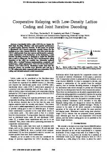
To validate our analysis, we compare the analytical results, which are obtained by using the average BER closed-form expression, with the simulation results obtained through Monte Carlo simulation. For each run of the Monte Carlo simulation, two symbols, a 2 × 2 MIMO channel matrix (i.e., the MIMO channel matrix between the transmitter and the receiver) and a 2 × 2 noise matrix (i.e., the noises generated at the receive antennas in the first and second time slots) are randomly generated. The number of Monte Carlo runs is chosen to be very large in order to accurately produce the average BER curve. In Figure 3.1, the average BER of Alamouti coding for BPSK is plotted ten times, and in each time the number of runs is 106 . The sold line represents the exact average BER, while the scattered points represent the Monte Carlo simulation for 106 runs. We can see that the simulation results, even with only 106 runs, exhibits low variance and closely match the theoretical results. Throughout the thesis, we run the Monte Carlo for 5 × 106 times (i.e., 107 symbols are gener39


10−1

10−2

BER

10−3

10−4

10−5

0

2

4

6 8 SNR (dB)

10

12

14

Figure 3.1: Average BER of Alamouti coding for BPSK. ated), which is large enough to obtain accurate average BER up to 10−5 through Monte Carlo simulation. Figure 3.2 shows the analytical and the simulation results of the average BER of the Alamouti code for BPSK, 4-QAM and 16-QAM. As expected, the analytical results have excellent agreement with the simulation results. In the BPSK case, the analytical results perfectly match the simulation results, because each symbol conveys only one bit, so the average BER is exactly equal to the Al Al average SER (i.e., P¯b,k→R = P¯s,k→R ). In the M -QAM case, at low SNR, there

is an error between the analytical and simulation results due mainly to the approximation in (3.10). This error decreases either as the modulation order decreases or the SNR increases. 40

3.3. BER of the MMSE Detector

100 Theoretical: 16-QAM Simulation: 16-QAM Theoretical: 4-QAM Simulation: 4-QAM Theoretical: BPSK Simulation: BPSK

10−1

BER

10−2

10−3

10−4

10−5 0

2

4

6

8

10

12 γ¯k,R

14 (dB)

16

18

20

22

24

Figure 3.2: BER performance of the point-to-point Alamouti coding.

3.3

BER of the MMSE Detector

In this section we derive an approximate closed-form BER expression for the MMSE detector presented in Section 2.5. Let P MMSE (γk,R ) denote the instantas neous SER of detecting the symbol xk,v at the relay which, for square M -QAM, can be approximated as [64]

P MMSE (γk,R ) ≈ α Q s

where α = 4(1 −

√1 ), M

and β =

3 . 2(M −1)

p 2βγk,R ,

(3.11)

The random value γk,R is the in-

stantaneous signal-to-interference-plus-noise ratio (SINR) of xk,v at the MMSE 41


detector output at the relay, and is given by (see details in Appendix A.2)

γk,R =

Ek H hk,v M−1 l hk,v , 2

(3.12)

where hk,v is the v th column of the effective channel matrix Hk and Ml = El Hl HlH 2

2 + σN I4 (where l 6= k) is the interference-pulse-noise covariance matrix.

Because of the structure of the Alamouti STBC, we have γk,1,R = γk,2,R = γk,R . Using spectral decomposition we can rewrite Ml as Ml = Vl Λl VlH ,

(3.13)

where Λl and is a diagonal matrix of the eigenvalues of Ml , and Vl is the eigenvector matrix. According to [67], the eigenvalues of Ml are given by

λl,n

   2  σ  N 1+    2 = σN 1+       2 σN ,

where γl,v =

γl,1 +γl,2 2 γl,1 +γl,2 2

p (γl,1 − γl,2 )2 + 4ρ12 , p − 12 (γl,1 − γl,2 )2 + 4ρ12 , +

1 2

n=1 n=2

,

(3.14)

n = 3, 4

El H 2 hl,v hl,v 2σN

=

El 2 2σN

kHl k2F is the instantaneous SNR of the symbol

xl,v , which has a chi-square distribution with eight degrees of freedom, and ρ12 = 2 | 2σEl2 hH l,1 hl,2 | = 0 because hl,1 and hl,2 are orthogonal. Therefore, (3.14) can be N

rewritten as λl,n =

   2  El kHl k2F + σN , 2

n = 1, 2

  2 σ N ,

n = 3, 4 42

.

(3.15)


Using (3.13) we can express (3.12) as

γk,R =

Ek H −1 u Λ uk,v , 2 k,v l

(3.16)

where the vector uk,v = VlH hk,v = [uk,v,1 , uk,v,2 , uk,v,3 , uk,v,4 ]T has the same probability density function of hk,v , because Vl is a unitary matrix (i.e., Vl VlH = VlH Vl = I). We can rewrite (3.16) as

γk,R

L X Ek |uk,v,n |2 , = 2λl,n n=1

(3.17)

where L = 4 is the number of independent channels between Ak

The average SER of detecting a symbol from Ak at the relay is found by averaging (3.1) over the pdf of γk,R and the pdf of λl,1 . Because it is difficult to take the average over the pdf of λl,1 , we use the average value of λl,1 , which is given by

¯ l,1 = E [λl,1 ] = 2El σ 2 + σ 2 . λ l N

(3.18)

Therefore, the average SER of detecting a symbol from Ak at the relay can be expressed as [66] α MMSE P¯s,k→R ≈ π

ˆ

π/2

Φγk,R

0

2β − 2 sin2 (θ)

dθ,

(3.19)

where Φγk,R (ω) is the MGF of γk,R and is given by Φγk,R (ω) =

1 1 − ω¯ γk,R

L−Ns

1 γ ¯ 1 − ω λ¯l,1k,R /σ 2

N

43

!Ns ,

(3.20)


where γ¯k,R =

σk2 Ek 2 2σN

is the average SNR per channel per symbol, L = 4 is the

number of independent channels between Ak and the relay and Ns = 2 is the number of interfering symbols. Then, (3.19) can be rewritten as

MMSE P¯s,k→R

where ψ1 = β¯ γk,R , ψ2 =

α ≈ π

ˆ

π/2

2 Y

0

β¯ γk,R ¯ l,1 /σ 2 , λ N

l=1

sin2 (θ) sin2 (θ) − ψl

ml dθ,

(3.21)

m1 = L − Ns and m2 = Ns .

Using the results of the limit integral in [66], an approximate closed-form MMSE expression for P¯s,k→R is

MMSE P¯s,k→R

Ns −1 " # L−N N s −1 s −1 α ψψ12 X X ψ1 Cm Im (ψ1 ) , (3.22) ≈ Bm Im (ψ2 ) − L−1 ψ ψ1 2 m=0 m=0 2 1 − ψ2

where

Bm =

ψ2 ψ1

m −1

m NX s −1 ψ1 Cm = 1 − ψ2 n=0 Am = (−1)

Ns −1+m

and

(Ns − 1)!

s Im (ψ) = 1 −

Ns −1 m

Am

,

(3.23)

m n An , L−1 n

(3.24)

L−1 m

Ns Y

(L − n) ,

(3.25)

n=1 n6=m+1

m ψ X 2n [4 (1 + ψ)]−n . 1 + ψ n=0 n

(3.26)

Using the well-known approximation in [64], the BER is given by

MMSE P¯b,k→R ≈

44

MMSE P¯s,k→R . log2 M

(3.27)


100

10−1

BER

10−2

10−3 Theoretical: 16-QAM Simulation: 16-QAM Theoretical: 4-QAM Simulation: 4-QAM Theoretical: BPSK Simulation: BPSK

10−4

10−5 0

2

4

6

8

10 12 14 16 18 20 22 24 26 28 30 γ¯1,R (dB)

Figure 3.3: BER performance of the MMSE detector for γ¯2 = γ¯1 . This approximate closed-form expression of the average BER can also be used for any other modulation scheme that has instantaneous SER in the form p of α Q 2βγk,R . To confirm our analysis, the average BER results obtained by using (3.27) are compared with the average BER results obtained thorough Monte Carlo simulation. In Figure 3.3 shows the analytical and the simulation results of the average BER performance of the MMSE detector for BPSK, 4-QAM and 16-QAM. We consider the case where the average SNR between node A2 and the relay is equal to the average SNR between node A1 and the relay (i.e, γ¯1,R = γ¯2,R ). As expected, the analytical results are very close to the simulation results.

45


100

10−1

BER

10−2

10−3 Theoretical: 16-QAM Simulation: 16-QAM Theoretical: 4-QAM Simulation: 4-QAM Theoretical: BPSK Simulation: BPSK

10−4

10−5 0

2

4

6

8

10 12 14 16 18 20 22 24 26 28 30 γ¯1,R (dB)

Figure 3.4: BER performance of the MMSE detector for γ¯2 = 15 dB. In Figure 3.4, we extend the simulation to the case when γ¯2,R = 15 dB, and γ¯1,R varies from 0 dB to 30 dB. As shown in the figure, the analytical results agree with the simulation results, and at high SNR they have very good match.

3.4

BER of Four-Phase Relaying

In this section we evaluate the average end-to-end BER for the four-phase relaying scheme. The average end-to-end BER is defined as the average BER of detecting the transmitted bits from node Ak at node Al , where k, l ∈ {1, 2} and k 6= l. 46

3.4. BER of Four-Phase Relaying

In the four-phase relaying scheme, as described in Chapter 2, node Ak transmits its symbol vector to node Al over two independent wireless links; the first link is from node Ak to the relay (Ak → R) and the second link is from the relay to node Al (R → Al ). These two links have independent BER, because the symbol vector transmitted from Ak is detected (i.e., hard-estimated) at the relay, then the relay transmits the detected symbol vector to Al . As a result, the average end-to-end BER can be calculated as

Al Al Al Al P¯b,k→l = P¯b,k→R P¯b,R→l 1 − P¯b,R→l + 1 − P¯b,k→R Al Al Al Al = P¯b,k→R + P¯b,R→l − 2P¯b,k→R P¯b,R→l ,

(3.28)

Al is the average BER of the Ak → R link (i.e, BER of the first hop) where P¯b,k→R Al and P¯b,R→l is the average BER of the R → Al link (i.e, BER of the second hop).

The end-to-end bit error occurs if and only if a bit error happens either in the Ak → R or in the R → Al link, but not both. If a bit error happens in both links, Al will correctly receive the transmitted bit from Ak .

To validate our analysis, the average end-to-end BER results obtained by using (3.28) are compared with the average BER results obtained thorough Monte Carlo simulation. Figure 3.5 shows the analytical and the simulation results of the average end-to-end BER performance of the four-phase detectand-forward relaying scheme for BPSK, 4-QAM and 16-QAM. We consider the average SNR between node A2 and the relay is equal to the average SNR between node A1 and the relay (i.e, γ¯1,R = γ¯2,R ). As expected, the analytical results are very close to the simulation results. 47


100 Analytical: 16-QAM Simulation: 16-QAM Analytical: 4-QAM Simulation: 4-QAM Analytical: BPSK Simulation: BPSK

10−1

BER

10−2

10−3

10−4

10−5 0

2

4

6

8

10

12 14 γ¯1,R

16

18

20

22

24

26

Figure 3.5: End-to-end BER performance of the four-phase detect-andforward relaying scheme for γ¯2,R = γ¯1,R .

3.5

BER of Three-Phase Relaying

In this section we derive the average end-to-end BER for the three-phase relaying scheme when the relay either uses the XOR-and-forward strategy or the detectand-forward strategy.

3.5.1

XOR-and-Forward strategy

In the XOR-and-forward strategy, as discussed in the Chapter 2, the relay uses a bitwise-XOR operation to combine the detected symbols, and at node Al the receiver applies the bitwise-XOR operation to its original transmitted bit and 48

3.5. BER of Three-Phase Relaying

the detected bit to extract the transmitted bit from Ak . As a results, the average end-to-end BER of detecting the transmitted bit from Ak at Al depends on the BER of the detecting the transmitted bit from Al at the relay. In other words, an end-to-end bit error occurs if and only if a bit error happens in one of the Ak → R, Al → R or the R → Al links or all three. Otherwise, Al will correctly receive the transmitted bit from Ak . Therefore, the average end-to-end BER of the transmitted bit from Ak at Al can be expressed as Al Al Al P¯b,k→l = P¯b,k→R 1 − P¯b,l→R 1 − P¯b,R→l Al Al Al + 1 − P¯b,k→R P¯b,l→R 1 − P¯b,R→l Al Al Al + 1 − P¯b,k→R 1 − P¯b,l→R P¯b,R→l Al Al Al +P¯b,k→R P¯b,l→R P¯b,R→l .

(3.29)

The average SNR of between node Ak and the relay depends on the location of the node and the relay, which varies slowly. For this reason, we assume the average SNR between node Ak and the relay remains constant over the period of the communication between the nodes. Therefore, the average BER of Al → R Al Al link is equals to the average BER of R → Al link (i.e., P¯b,l→R = P¯b,R→l ), and

(3.29) can be simplified to

Al Al Al Al P¯b,k→l = P¯b,k→R + 2 P¯b,l→R − 4 P¯b,k→R P¯b,l→R 2 2 Al Al Al . −2 P¯b,l→R + 4 P¯b,k→R P¯b,l→R

(3.30)

To validate our analysis, the average end-to-end BER results obtained by using (3.29) are compared with the average BER results obtained thorough Monte Carlo simulation. Figure 3.6 shows the analytical and simulation results 49



10−1

BER

10−2

10−3

10−4

10−5 0

2

4

6

8

10

12 14 γ¯1,R

16

18

20

22

24

Figure 3.6: A1 → A2 average BER performance of the three-phase XOR-andforward relaying scheme for γ¯2,R = γ¯1,R + 5 dB. of the A1 → A2 average BER performance of the three-phase detect-and-forward relaying scheme for BPSK, 4-QAM and 16-QAM. We consider the case where the average SNR between node A2 and the relay is equal to the average SNR between node A1 and the relay plus 5 dB(i.e, γ¯2,R = γ¯1,R + 5 dB). As expected, the analytical results show an excellent agreement with the simulation results.

3.5.2

Detect-and-forward strategy

In the detect-and-forward strategy the relay linearly combines the detected symbols. As a results, the average end-to-end BER of detecting the symbol of node Ak at node Al is affected by the SER of detecting the symbol xˆl,v at the relay, 50


because node Al subtracts its original transmitted symbol xl,v from the received sample to remove its effect (i.e., self-interference) as shown in (2.22). If the relay detects the transmitted symbol xl,v correctly, (i.e., xˆl,v = xl,v ), node Al can remove the self-interference completely from the received sample, otherwise, node Al cannot cancel the self-interference. To evaluate the average end-to-end BER of detecting the transmitted bits from Ak at Al , we need to evaluate the average BER of the Ak → R and R → Al links. The average BER for the Ak → R link is already derived in Section 3.2 and is given by (3.10). To evaluate the average BER of the R → Al link, we first evaluate the average SER of detecting the symbol xˆk,v at node Al . We use the total probability theorem [68] to calculate the average probability of correctly detecting the symbol xˆk,v given that xˆk,v = sm3 is transmitted from the relay, which can be expressed as

Pr[xˆˆk,v = sm3 |ˆ xk,v =sm3 ] =

M X

Pr[xl,v = sm1 , xˆl,v = sm2 , xˆˆk,v = sm3 |ˆ xk,v = sm3 ]

m1 =1 m2=1

=

M X

Pr[xl,v = sm1 |, xˆk,v = sm3 ]

m1 =1 m2=1

× Pr[ˆ xl,v = sm2 |xl,v = sm1 , xˆk,v = sm3 ] × Pr[xˆˆk,v = sm3 |xl,v = sm1 , xˆl,v = sm2 , xˆk,v = sm3 ].

(3.31)

Because xl,v and xˆk,v are independent and xˆl,v and xˆk,v are independent, then the probability of occurrence of the symbols xl,v and xˆl,v are not affected by the 51


occurrence of the symbol xˆk,v . Therefore, (3.31) can be simplified to Pr[xˆˆk,v = sm3 |ˆ xk,v =sm3 ] =

M X

Pr[xl,v = sm1 ] Pr[ˆ xl,v = sm2 |xl,v = sm1 ]

m1 =1 m2 =1

× Pr[xˆˆk,v = sm3 |xl,v = sm1 , xˆl,v = sm2 , xˆk,v = sm3 ],

(3.32)

where Pr[xl,v = sm1 ] is the probability of xl,v = sm1 to be transmitted from Al . Since M -QAM is used and the symbols are equally likely to be transmitted, then Pr[xl,v = sm1 ] =

1 M

. Pr[ˆ xl,v = sm2 |xl,v = sm1 ] denotes the transition probability

that xˆl,v = sm2 is detected at the relay given that xl,v = sm1 is transmitted from Al . Pr[xˆˆk,v = sm3 |xl,v = sm1 , xˆl,v = sm2 , xˆk,v = sm3 ] denotes the probability that xˆk,v = sm3 is detected correctly at Al given that xl,v = sm1 is transmitted from Al and xˆl,v = sm2 is detected at the relay. The approximate average SER of detecting the symbol xˆk,v at node Al is given by

P¯s,R→l = 1 −

M X

Pr[xˆˆk,v = sm3 |ˆ xk,v = sm3 ] Pr[ˆ xk,v = sm3 ]

m3 =1 M 1 X Pr[xˆˆk,v = sm3 |ˆ xk,v = sm3 ], =1− M m =1

(3.33)

3

since all the symbols are equally likely to be transmitted, so Pr[ˆ xk,v = sm3 ] =

1 . M

With Gray coding, the BER can be approximated by P¯s,R→l P¯b,R→l ≈ . log2 M

(3.34)

The average end-to-end BER of detecting the transmitted bit from Ak at Al 52


can be expressed as

Al Al P¯b,k→l = P¯b,k→R 1 − P¯b,R→l + 1 − P¯b,k→R P¯b,R→l Al Al + P¯b,R→l − 2P¯b,k→R P¯b,R→l . = P¯b,k→R

(3.35)

Similar to the four-phase detect-and-forward relaying, the end-to-end bit error occurs if and only if a bit error happens either in the Ak → R or in the R → Al link, but not both. If a bit error happens in both links, Al will correctly receive the transmitted bit from Ak . In the following we give an example to illustrate how to evaluate the probability of correctly detecting the symbol xˆk,v at node Al .

Example:

In this example, we illustrate how to evaluate the average BER for the R → Al link. We consider the case where the nodes and the relay uses BPSK to transmits their bits. The signal constellation for BPSK is shown in Figure 3.7, where symbol s1 and s2 are located at d and −d, respectively, where d = 1 for BPSK which results in a covariance matrix of I2 (i.e., Rxk = E xk xk = I2 , see (2.3)). The decision region for symbol s1 is shown by the shaded area, while the decision region for s2 is shown by the unshaded area. We use the notation Dm to denote the the decision region for symbol si. The transition probability, for the BPSK, is the probability that xˆl,v = sm2 is detected when xl,v = sm1 is transmitted, and is given by 53


D2

D1

s2

s1

-d

d

Re

Figure 3.7: The signal constellation of BPSK. s1 = d and s2 = −d.

Pr[ˆ xl,v = sm2 |xl,v

where E[Q(

  p  2  2d γk,R , E Q = sm1 ] = p   2  2d γk,R , 1 − E Q

m1 6= m2 ,

(3.36)

m1 = m2

p 2d2 γR,l ) is the average SER of Alamouti coding for BPSK, and

is given (3.8) for α = 1 and β = d2 . As shown in Section 2.4, node Al multiplies the received sample by a weight matrix and then subtracts its original transmitted vector from the result of the multiplication. The result of these operation can be written as

m3 x˜˜k = ξm +n ˜l, 2 ,m1

(3.37)

m3 where ξm is a new constellation points as shown in Figure 3.8,which result 2 ,m1

from the the subtraction (self-interference cancellation) and is given by r m3 ξm 2 ,m1

= sm 3 + 54

δl sm2 − sm1 . δk

(3.38)


2 ξ2,1

D2

D1

2 ξ2,2 2 ξ1,1

1 ξ2,2 1 ξ1,1

2 ξ1,2

1 ξ2,1

1 ξ1,2

Re

(a) δ1 > 2δ2

D2

2 ξ2,1

2 ξ2,2 2 ξ1,1

D1

1 ξ2,1

2 ξ1,2

1 ξ2,2 1 ξ1,1

1 ξ1,2

Re

(b) δ1 < 2δ2

xˆ1 = s1

xˆ1 = s2 .

Figure 3.8: The signal constellation after self-interference cancellation at node Al .

55


The error probability of detecting the transmitted symbol from node Ak at node Al is affected by the new constellation point, i.e., the probability of error m3 is high for ξm located close to the boundary decision. For example, consider 2 ,m1

the detected symbols of node A1 and A2 at the relay are xˆ1,v = s1 , xˆ2,v = s2 , respectively, and the transmitted symbol from node A2 is x2,v = s1 , which q q δl 1 results in ξ2,1 = s1 + δk (s2 − s1 ) = d + δδkl (−2d). Therefore, the probability 1 is close of detecting the symbol xˆ1,v at node A2 is high, because the point ξ2,1

to the boundary decision. So, the probability of correct detection at node Al , when xk,v = sm3 , xl,v = sm1 and xl,v = sm2 , is given by

Pr[xˆˆk,v = sm3 |xl,v = sm1 , xˆl,v = sm2 , xˆk,v = sm3 ] =

   1 − f,

m3 ξm ∈ / Dm3 2 ,m1

  f,

m3 ξm 2 ,m1

,

∈ Dm3 (3.39)

where q m3 2γR,l |ξm2 ,m1 |2 f = E Q

(3.40)

and r m3 ξm 2 ,m1

= sm 3 +

δl (sm2 − sm1 ). δk

(3.41)

p m3 2 where E[Q( 2γR,l |ξm 2 ,m1 | ) is the average SER of Alamouti coding for BPSK, m 2 3 . and is given by (3.8) for α = 1 and β = ξm 2 ,m1 In the following, we extend the example to 4-PAM case. As shown in Figure 3.9, the symbol are arranged on the real axis, and the symbol sm has value of (M + 1 − 2m)d, where 2d is the minimum distance between two adjacent 56


D4

D3

D2

D1

s4

s3

s2

s1

−3d

−d

d

3d

Re

Figure 3.9: The signal constellation of 4-PAM. The dashed lines denotes the boundary of the decision regions.

symbols and is given by d =

q

3 M 2 −1

for Rxk = E xk xk = I2 . The decision

region boundaries, which divide the decision regions between of two adjacent symbols, are given by (M − 2m)d for m ∈ {1, 2, · · · , M − 1}. The transition probability, for the 4-PAK, when xˆl,v = sm2 is detected and xl,v = sm1 is transmitted can be evaluated as

Pr[ˆ xl,v = sm2 |xl,v = sm1 ] =

    1 − q1        1 − 2q

for m2 = m1 , m2 ∈ {1, M } for m2 = m1 , m2 ∈ {2, 3 · · · , M − 1}

1

   qθ        qθ − qθ+1

for m2 6= m1 , m2 ∈ {1, M } for m2 6= m1 , m2 ∈ {2, 3 · · · , M − 1} (3.42)

q 2 where θ = |m1 − m2 | and qθ = E Q( 2 (2θ − 1)d γR,l ) . The probability of correct detection at node Al , when xk,v = sm3 , xl,v = sm1 and xl,v = sm2 , is given by 57

,


Pr[xˆˆk,v = sm3 |xl,v = sm1 , xˆl,v = sm2 , xˆk,v = sm3 ] =

   fUm3 + fLm3 ,

m3 ξm ∈ / Dm3 2 ,m1

  1 − fUm3 − fLm3 ,

m3 ξm 2 ,m1

,

∈ Dm3

(3.43) where q m3 = E Q 2γR,l |(M − 2m3 ) − ξm2 ,m1 |2

(3.44)

q m3 = E Q 2γR,l |(M + 2 − 2m3 ) − ξm2 ,m1 |2 ,

(3.45)

fUm3

and

fLm3

are the upper an lower boundaries for the decision region of the symbol sm3 (i.e., Dm3 ). The upper boundary for the decision region D1 is infinity, so fU1 = 0 for s1 , and the lower bound for the decision region DM is minus infinity, so fLM = 0 for sM , because Q(∞) = 0.

Now, we extend the example to the squared M -QAM case. Unlike the M PAM in which each symbol is represented by a real number, the M -QAM is a two dimensional mapper, in which each symbol is represented by a complex number (i.e., real and the imaginary), as shown in Figure 3.10. It can be noted √ that the M -QAM constellation can be generated by combining two M -PAM q with d = 2(M3−1) , one in the real axis and the other on the imaginary axis. Therefore, the square M -QAM symbol can be represented as

sm = zmRe + j zmIm , 58

(3.46)


Im

−3d

−d

d

3d

Re

Im

3d

3d

d

d

=

+

−3d

−d

d

−d

−d

−3d

−3d

3d

Re

Figure 3.10: The signal constellation of 16-QAM.

where zmRe and zmIm are the √ Note that j = −1 .

√

M -PAM symbols and mRe , mIm ∈ {1, 2, · · · ,

√

M }.

The transition probability, for the M -QAM, when xˆl,v = sm2 is detected and xl,v = sm1 is transmitted can be evaluated as Re Pr[ˆ xl,v = sm2 |xl,v = sm1 ] = Pr[ˆ xRe l,v = zmRe,2 |xl,v = zmRe,1 ]

(3.47)

Im × Pr[ˆ xIm l,v = zmIm,2 |xl,v = zmIm,1 ],

Re Im where Pr[ˆ xRe xIm l,v = zmRe,2 |xl,v = zmRe,1 ] and Pr[ˆ l,v = zmIm,2 |xl,v = zmIm,1 ] can be

evaluated by using (3.42). To validate our analysis, the average end-to-end BER results obtained by using (3.35) are compared with the average BER results obtained through Monte Carlo simulation. Figure 3.11 shows the analytical and simulation results of the A1 → A2 average BER performance of the three-phase detect-and-forward relaying scheme for BPSK, 4-QAM and 16-QAM. We consider the case where the average SNR between node A2 and the relay is equal to the average SNR between node A1 and the relay plus 5 dB(i.e, γ¯2,R = γ¯1,R + 5 dB). We also 59



10−1

BER

10−2

10−3

10−4

10−5 0

2

4

6

8

10

12 14 γ¯1,R

16

18

20

22

24

Figure 3.11: A1 → A2 average BER performance of the Three-phase detectand-forward relaying scheme for γ¯2,R = γ¯1,R + 5 dB and δ1 = 0.7. consider the power-splitting factor δ = 0.7 (i.e., δ1 = 0.7 and δ2 = 0.3). As expected, the analytical results show an excellent agreement with the simulation results.

3.6

BER of Two-Phase Relaying

In this section, we derive the average end-to-end BER for the two-phase relaying scheme when the relay uses either the XOR-and-forward or the detect-andforward strategy. We consider the case where relay uses the MMSE detector to estimate the symbols transmitted from the nodes. 60

3.6. BER of Two-Phase Relaying

3.6.1

XOR-and-Forward strategy

In two-phase relaying using the XOR-and-forward strategy, as discussed in the Chapter 2, the relay uses a MMSE detector to detect the transmitted symbols from the nodes, then uses the bitwise-XOR operation to combine the detected symbols. The average end-to-end BER derivation for two-phase relaying, when the XOR-and-forward strategy is used, is similar to the derivation of threephase relaying in Section 3.5.1, except the node-to-relay BER is given by (3.27) instead of (3.10). Therefore, the end-to-end average BER is

MMSE MMSE Al P¯b,k→l = P¯b,k→R 1 − P¯b,l→R 1 − P¯b,R→l Al MMSE ¯ MMSE Pb,l→R 1 − P¯b,R→l + 1 − P¯b,k→R MMSE MMSE ¯ Al + 1 − P¯b,k→R 1 − P¯b,l→R Pb,R→l MMSE ¯ MMSE ¯ Al +P¯b,k→R Pb,l→R Pb,R→l .

(3.48)

To validate our analysis, the average end-to-end BER results obtained by using (3.48) are compared with the average BER results obtained through Monte Carlo simulation. Figure 3.12 shows the analytical and simulation results of the A1 → A2 average BER performance of the three-phase detect-and-forward relaying scheme for BPSK, 4-QAM and 16-QAM. We consider the case where the average SNR between node A2 and the relay is equal to the average SNR between node A1 and the relay plus 5 dB (i.e, γ¯2,R = γ¯1,R + 5 dB). As expected, the analytical results show an excellent agreement with the simulation results. 61


100

10−1

BER

10−2

10−3 Analytical: 16-QAM Simulation: 16-QAM Analytical: 4-QAM Simulation: 4-QAM Analytical: BPSK Simulation: BPSK

10−4

10−5 0

2

4

6

8

10 12 14 16 18 20 22 24 26 28 30 γ¯1,R

Figure 3.12: A1 → A2 average BER performance of the two-phase XOR-andforward relaying scheme for γ¯2,R = γ¯1,R + 5 dB.

3.6.2

Detect-and-forward strategy

The derivation of the BER of the detect-and-forward strategy for two-phase relaying is similar to the three-phase relaying in Section 3.5.2. The average end-to-end average BER is given by

MMSE MMSE ¯ P¯b,k→l = P¯b,k→R 1 − P¯b,R→l + 1 − P¯b,k→R Pb,R→l ,

(3.49)

MMSE where P¯b,k→R and P¯b,R→l are given by (3.27) and (3.34), respectively.

To validate our analysis, the average end-to-end BER results obtained by using (3.49) are compared with the average BER results obtained through Monte 62

3.6. BER of Two-Phase Relaying

100

10−1

BER

10−2

10−3 Analytical: 16-QAM Simulation: 16-QAM Analytical: 4-QAM Simulation: 4-QAM Analytical: BPSK Simulation: BPSK

10−4

10−5 0

2

4

6

8

10 12 14 16 18 20 22 24 26 28 30 γ¯1,R

Figure 3.13: A1 → A2 average BER performance of the two-phase detect-andforward relaying scheme for γ¯2,R = γ¯1,R + 5 dB. Carlo simulation. Figure 3.13 shows the analytical and simulation results of the A1 → A2 average BER performance of the two-phase detect-and-forward relaying scheme for BPSK, 4-QAM and 16-QAM. We consider the case where the average SNR between node A2 and the relay is equal to the average SNR between node A1 and the relay plus 5 dB (i.e, γ¯2,R = γ¯1,R + 5 dB). We also consider the power-splitting factor δ = 0.7 (i.e., δ1 = 0.7 and δ2 = 0.3). As expected, the analytical results show an excellent agreement with the simulation results.

63

Chapter

4

Performance Evaluation and Discussion In this chapter we evaluate and compare the performance of proposed two-way relaying schemes using the Monte Carlo method. This chapter is organized as follows. Firstly, we introduce the sum capacity measure which is used to evaluate the performance of the proposed two-way relaying schemes. Secondly, we simulate the end-to-end BER and the sum capacity of the proposed four-phase, threephase and two-phase relaying schemes and compare their performance. We also estimate and compare the energy consumption for these schemes. Thirdly, we investigate and compare the performance and computational complexity of the two-phase relaying schemes when the relay uses different detectors (i.e., MMSE, ZF, MMSE-OSIC, ZF-OSIC, and ML detectors). Lastly, we investigate the effect of the power-splitting factor on the performance of the detect-and-forward strategy. Throughout this chapter, we assume uncorrelated slow flat Rayleigh fading channels between node Ak and the relay, (Hk , Gk ), wherein the elements in these 64

4.1. Sum Capacity Performance channel matrices are modeled as iid ZMCG random variables with variance σk2 . We also assume that the CSI is perfectly known at the receivers of the nodes and the relay. Furthermore, the noises at the nodes and the relay are modeled 2 as iid ZMCG with variance σN . The average SNR of the Ak → R link is given

by γ¯k,R = σk2 σE2k , and the average SNR of the R → Ak link given by γ¯R,k = σk2 σE2k . N

N

We assume the average transmit energy per time slot of the relay and nodes to be equal (i.e., E1 = E2 = ER ).

4.1

Sum Capacity Performance

In this section we introduce the sum capacity performance, which is used to evaluate and compare the proposed two-way relaying schemes. The sum capacity is defined as the sum of the end-to-end maximum achievable date rate of the two nodes when a good error correction code is applied. Most of the researchers uses the Shannon capacity formula, which is a function of SNR, to evaluate the sum capacity performance of the relaying systems. The Shannon capacity considers the input and the output of the digital communication systems to the system be is continuous-values with Gaussian distribution. However, in these systems (i.e., digital communication systems), the input to the systems is represented as discrete-values, since the transmitter maps a binary sequence to symbols, and the output can be represented as discrete-values or a continuous-values depends on the decoder (i.e., the output is discrete-values for the hard decoder and the output is continuous-values for the soft decoder). The channel capacity for the discrete-input discrete-output system can be calculated using either the conventional method [69] or the log-likelihood ratio (LLR) [70,71]. The conventional method is symbol-based, in which the input to 65

Chapter 4. Performance Evaluation and Discussion

the system is considered to be symbols. while the LLR method is bit-based, in which the input to the system is considered to be bits. However, the capacity of the LLR method is equal to the capacity of the conventional method only when BPSK or 4-QAM is used, because the LLR method depends on the constellation ordering (e.g. Gray coding order, binary order). For simplicity, we use the discrete-input discrete-output method to calculate the capacity of the proposed two-way relaying schemes. The end-to-end capacity (i.e., Ak → Al , k, l = 1, 2 and l 6= k) is given by

Ck

ˆ ˆ = H(xˆk,v ) − H xˆk,v |xk,v ,

(4.1)

where H(xˆˆk,v ) is the entropy of xˆˆk,v , where xˆˆk,v is the detected symbol of node ˆ Ak at node Al and is random variable. H xˆk,v |xk is the conditional entropy of xˆˆk,v detected at Al when xk,v is transmitted from Ak , and is given by M X ˆ Pr[xk,v = sm1 ] H xˆˆk,v |xk,v = sm1 , H xˆk,v |xk,v =

(4.2)

m1 =1

where M X H xˆˆk,v |xk,v = sm1 = − Pr xˆˆk,v = sm2 |xk,v = sm1 m2 =1

× log2 Pr xˆˆk,v = sm2 |xk,v = sm1 .

(4.3)

The probability distribution of xˆˆk is uniform distribution, since xk has a uniform distribution. Therefore, we can express (4.1) as Ck = log2 (M ) − H xˆˆk |xk , 66

(4.4)

4.2. Two-way Relaying Schemes

where M is the modulation order (i.e., the number of the different symbol values). Therefore, the sum capacity for a two-way relaying system with a good error correction code is

Csum =

2 X

Ck

k=1

4.2

Two-way Relaying Schemes

In this section we investigate and compare the performance of the proposed schemes, which are presented in Chapter 3. We also investigate the energy consumption and the impact of the link quality on the proposed schemes. We consider the case where relay, in the two-phase relaying scheme, uses the MMSE detector. The performance of the two-phase relaying scheme when the relay uses the other detectors (i.e., ZF, OSIC and ML) are investigated and compared later. We consider the case when the power splitting-factor δ = 0.5 for the detect-and-forward strategy in the two-phase and three-phase relaying schemes.

4.2.1

Performance Comparison

In this section we evaluate and compare the performance of the proposed twoway relaying schemes. In Figure 4.1 we plot the end-to-end average BER (i.e., A1 → A2 average BER) for the proposed schemes for a spectral efficiency of 4 bit/s/Hz, i.e. the four-phase, the three-phase and the two-phase relaying schemes use 256-QAM, 64-QAM and 16-QAM, respectively. We assume the average SNR between node A2 and the relay is equal to the average SNR between node A1 and the relay, i.e., γ¯2,R = γ¯1,R and γ¯k,R = γ¯R,k . As expected, the two-phase relaying scheme 67


100

10−1

BER

10−2

10−3

Two-phase XF relaying Two-phase DF relaying Three-phase XF relaying Three-phase DF relaying Four-phase DF relaying

10−4

10−5 0

2

4

6

8

10 12 14 16 18 20 22 24 26 28 30 γ¯1,R

Figure 4.1: The end-to-end average BER of the proposed two-way relaying schemes for a spectrum efficiency of 4 bit/s/Hz. The relay uses MMSE detector for two-phase relaying. δ = 0.5 for DF strategy. outperforms the three-phase and four-phase relaying schemes at low SNR, because it uses a lower modulation order i.e., lower number of constellation points. But at high SNR the two-phase relaying scheme has worse BER performance than the three-phase and four-phase relaying schemes, because the three-phase and four-phase relying schemes can provide higher diversity order than the two phase relaying scheme. As shown Figure 4.1, for the three-phase relaying schemes, the XOR-andforward strategy outperforms the detect-and-forward strategy. This is because, in the detect-and-forward strategy, the relay splits the power between the two detected symbol vectors, which results in a higher BER in the second link 68


(i.e., R → A2 link). In the two-phase scheme the performance of the detectand-forward and XOR-and-forward strategies are almost the same. The reason behind this is that the relay detects the transmitted symbols from the nodes with high probability of error, since the nodes simultaneously transmit their symbols to the relay. These errors significantly degrade the BER of the broadcast phase, because the nodes use their original symbols to remove the effect of self-interference from the received samples (see Section 2.5). If the relay uses the ML detector the BER of the Ak → R will be improved significantly, which results in the XOR-and-forward strategy is outperforming the detect-and-forward strategy as will be shown later. Figure 4.2 shows the sum capacity for the proposed schemes for the same previous configuration. As can be seen, the two-phase relaying provides higher sum capacity than the three-phase and four-phase relaying scheme at high SNR, although it uses a lower modulation order (16-QAM). At low SNR, the four-phase relaying scheme outperforms the two-phase and three-phase relaying schemes. However, the two-phase can relaying schemes can improve the sum capacity, at low SNR, by switching to a lower modulation order, for example 4-QAM or BPSK. In Figure 4.3, we plot and compare the maximum sum capacity for the proposed schemes. The maximum sum is defined as the maximum values of the sum capacities for different modulation orders (i.e., BPSK, 4-QAM, 16-QAM, 64-QAM and 256-QAM), and is obtained by generating sum capacity curves for different modulation order, and then taking the maximum values of these curves. In Figure 4.3, as expected the two-phase relaying can provide a higher capacity than the three-phase and four-phase relaying schemes. For example, at SNR of 30 dB the two-phase, three-phase and four-phase relaying can offer 69


4 3.5

Sum capacity (b/s/Hz)

3 2.5 2 1.5 Two-phase XF relaying Two-phase DF relaying Three-phase XF relaying Three-phase DF relaying Four-phase DF relaying

1 0.5 0

0

2

4

6

8

10 12 14 16 18 20 22 24 26 28 30 γ¯1,R

Figure 4.2: The sum capacity of the proposed two-way relaying schemes for a spectrum efficiency of 4 bit/s/Hz. The relay uses MMSE detector for two-phase relaying. δ = 0.5 for DF strategy.. a capacity of 7.2, 5.2 and 4 bit/s/Hz, respectively. We also see that the threephase XOR-and-forward scheme, at a SNR of 11 dB, provides slightly higher capacity than two-phase relaying. However, at this SNR the sum capacity of the two-phase scheme can be improved by using an optimal non-rectangular 8-QAM constellation.

4.2.2

Impact of Link Quality

In this section we investigate the impact of the link quality on the performance of the two-way relaying schemes. To do this, we plot the BER curves in each 70


8 Two-phase XF relaying Two-phase DF relaying Three-phase DF relaying Three-phase DF relaying Four-phase DF relaying

7

Sum capacity (b/s/Hz)

6 5 4 3 2 1 0

0

2

4

6

8

10 12 14 16 18 20 22 24 26 28 30 γ¯1,R

Figure 4.3: The maximum sum capacity of the proposed two-way relaying schemes. The relay uses MMSE detector for two-phase relaying. δ = 0.5 for DF strategy. ˆ k at phase, i.e., the BER of detecting bk at the relay, the BER of detecting b the node Al (k, l = 1, 2 and k 6= l) and the end-to-end BER. In this section, we consider the SNR between node A2 and the relay is fixed at γ¯2,R = 14 dB, while the SNR between node A1 and the relay varies. The nodes and the relay uses 4-QAM with Gray coding. Figure 4.4 shows the BER curves of detecting b1 and b2 at the relay for the four-phase, three-phases and two-phase relaying schemes. As can be seen, the four-phase and the three-phase relaying schemes have exactly the same BER performance, and outperform the two-phase relaying schemes. This is because, in the four-phase and three-phase schemes, the nodes transmit their symbols 71


100 Four-phase relaying Three-phase relaying Two-phase relaying

10−1

BER

10−2

10−3

10−4

10−5

0

2

4

6

8

10 12 14 16 18 20 22 24 26 28 30 γ¯1,R

Figure 4.4: The BER of detecting the bk at the relay. (solid lines: BER of b1 at the relay, BER of b2 at the relay)

over different phases, while in the two-phase schemes, the nodes simultaneously, in the same phase, transmit their symbols to the relay, causing the symbols interfere with each other at the relay. In the four-phase and three-phase schemes, the BER of detecting b2 is fixed at certain value because the average SNR between the relay and node A2 is fixed at 14 dB, while in the two-phase schemes the BER of b2 increases, because the average SNR between node A1 and the relay increases, i.e., the energy of the transmitted symbol from node A1 increases. ˆ 2 at node A2 and A1 , reˆ 1 and b In Figure 4.5 , we plot the BER of detecting b spectively, for four-phase, three-phase (i.e., using detect-and-forward and XORand-forward) and two-phase relaying schemes (i.e., using detect-and-forward 72


100 Two-phase XF relaying Two-phase DF relaying Three-phase XF relaying Three-phase DF relaying Four-phase DF relaying

10−1

BER

10−2

10−3

10−4

10−5

0

2

4

6

8

10 12 14 16 18 20 22 24 26 28 30 γ¯1,R

ˆ k at node Al . (Solid lines: BER of b ˆ1 Figure 4.5: The BER of detecting the b ˆ 2 at node A1 ). at node A2 , dashed lines: BER of b

and XOR-and-forward). As can be seen, the three-phase and two-phase schemes have higher BER than the four-phase scheme. Because the relay, in the threephase and the two-phase scheme, detects and combines/XORs the transmitted symbols/bits from the nodes, and node Al uses its original transmitted symbols/bits to cancel its effect (i.e., self-interference) from the received combined symbols/bits coming from the relay and estimate the symbols/bits transmitted from node Ak . Since errors may occur when the relay estimates the transmitted symbols/bits from node Al , these errors will increase the error probability of the symbols/bits of node Ak at node Al . Figure 4.6 shows the end-to-end BER curves of the four-phase, three-phase 73


100 Two-phase XF relaying Two-phase DF relaying Three-phase XF relaying Three-phase DF relaying Four-phase DF relaying

10−1

BER

10−2

10−3

10−4

10−5

0

2

4

6

8

10 12 14 16 18 20 22 24 26 28 30 γ¯1,R

Figure 4.6: The end-to-end average BER. (Solid lines: BER of b1 at node A2 , dashed lines: BER of b2 at node A1 ).

and two-phase relaying schemes. From the figure we observe that the performance of all schemes saturate at a certain values of BER (error floor), which results from the fixed value of the average SNR between node A2 and the relay (i.e., γ¯2,R ). The values of these error floors depends on the value of γ¯2,R and the modulation order. As expected from (3.28) the end-to-end BER for A1 → A2 and A2 → A1 links, for the four-phase scheme, are exactly the same. For threephase and two-phase schemes, the end-to-end BER for A1 → A2 and A2 → A1 links are different and depend on which link has the higher average SNR. For example, when γ¯1,R > γ¯2,R the BER of detecting the bits of node A1 at node A2 is worse than BER of detecting the bits of node A2 at node A1 , despite the 74


fact of that the bits of node A1 were transmitted over the higher SNR in the first hop. This issue occurs because node A2 use its original transmitted symbols/bits to remove its effect from the received combined symbols/bits coming from the relay and then estimate the symbols/bits coming from node A1 . For the XOR-and-forward strategy, the combined signal from the relay is composed of the estimated bits of node A1 and node A2 where the estimated bits of A2 (at the relay) has higher bit errors, these errors will increase the error probability of the bits A1 at node A2 . For the detect-and-forward strategy, the combined signal at the relay is composed of the estimated symbols (hard decision) of both nodes, where the estimated symbols of A2 (at the relay) has higher symbol errors, these symbol errors are treated as noise at node A2 , which results in a higher bit error probability of A1 at node Al .

4.2.3

Energy Consumption

In a relay network, users’ devices, such as smart-phones and laptops, may be deployed as mobile relays. Consequently, these types of relays have limited energy, since they use batteries to operate. Therefore, it is very important to investigate the energy consumption of the two-way relaying schemes, because the use of user’s devices as relays reduces the life-time of their batteries. As shown Figure 4.7 the relay transceiver has two main parts, the transmitter and the receiver. The transmitter consists of three main parts; the digital signal processing (DSP), digital-to-analog-converter (DAC), the up-converter (UC) and the power amplifier (PA), and receiver consists of the low-noise-amplifier (LNA), down-converter (DC), analog-digital-converter (ADC), and DSP. The DSP part of the receiver includes the detector and demapping, while the DSP 75


Transmitter DSP

DAC

Mixer

PA

Mixer

LNA

Receiver DSP

ADC

Figure 4.7: Block diagram of the relay transceiver. part of the transmitter includes the mapping and combining symbols, in the case of the two-phase and three-phase relaying schemes. The power amplifier consumes higher power than the other parts [72, 73]. The total power consumption of the relay, during transmission, is given by

PT x = PDDU + PP A ,

(4.5)

where PDDU is the combined power consumption of the DSP, DAC and upconverter, and PP A is the power consumption of the power amplifier. The consumption of the power amplifier depends on its efficiency ηP A , and is given by PP A =

PT , ηP A

(4.6)

where PT is the transmit power. In a similar way, the total power consumption of the relay, during the reception, is given by

PRx = PLN A + PDC + PADC + PDSPRx , 76

(4.7)


where PLN A , PDC , PADC and PDSPRx are the power consumption of the LNA, the down-converter, the ADC, and the DSP, respectively. In the four-phase relaying schemes, the nodes requires eight time slots to exchange four symbol, where the relay receives the transmitted symbols from nodes A1 and A2 in the first phase and third phase, respectively, and then forwards them to node A2 and A1 in the second and fourth phases, respectively. Therefore, the total energy consumption in the relay per two symbol duration is

E 4phase = 2Ts (2PT x + 2PRx ), = 4Ts (PDDU + PRX ) + 4Ts = 4Ts (PDDU + PRX ) + 4

PT ηP A

ET , ηP A

(4.8)

where Ts is the duration of one symbol (i.e., one time slot), and ET = Ts PT is the average transmitted energy per time slot at the relay, see Chapter 2 (i.e., ET = ER ). In the three-phase relaying schemes, the nodes requires six time slots to exchange four symbol, where the relay receives the transmitted symbols from nodes A1 and A2 in the first phase and second phase, respectively, and then broadcasts them to the nodes in the third phase. Therefore, the total energy consumption in the relay per two symbols duration is

E 3phase = 2Ts (PT x + 2PRx ) = 2Ts (PDDU + 2PRX ) + 2

ET . ηP A

(4.9)

In the two-phase relaying schemes, the nodes requires 4 time slots to ex77


change four symbol, where the relay receives the transmitted symbols from nodes A1 and A2 in the first phase, and then broadcasts them to the nodes in the second phase. Therefore, the total energy consumption in the relay per two symbols duration is

E 2phase = 2Ts (PT x + PRx ) = 2Ts (PDDU + PRX ) + 2

(4.10) ET . ηP A

(4.11)

In Figure 4.8, we plot the total energy consumption as a function of the average transmitted energy per time slot for the four-phase, three-phase and two-phase relaying schemes. We assume the power consumption in the receiver PRx = 100 mW, and the power consumption in the transmitter, without the power consumption in the power amplifier, PDDU = 100 mW. We also assume the symbol duration Ts = 1 µsec and the efficiency of the power amplifier ηP A =0.4 and we vary the transmit power (PT ) from 1 mW to 100 mW. As can be seen, the two-phase relaying schemes has the lower energy consumption than the four-phase and three-phase relaying schemes. Where at PT = 10 mW the two-phase can save energy of 0.45 mJ (50%) and 0.2 mJ (30.7%) compared with the four-phase and the three-phase schemes, respectively. While at PT = 100 mJ it can save energy of 0.9 mJ (50%) and 0.2 mJ (18.18%) compared with the fourphase and the three-phase schemes, respectively. These results were expected, since the relay, in the two-phase scheme, receives the transmitted symbols from the nodes in the first phase, and broadcast them in the second phase. In the four-phase scheme, the relay receives the transmitted symbols from the node on different phases, which increases the power consumption of the receiver, and the relay transmits the symbols to the node in different phase, which increases 78

4.3. Two-phase Relaying Detectors

1.8

(100, 1.8)

Four-phase Three-phase Two-phase

Total energy consumption (mJ)

1.6 1.4 1.2

(100, 1.1)

(10, 0.9)

1 0.8

(10, 0.65)

0.6

(10, 0.45)

0.4

0

10

20

(100, 0.9)

30

40 50 60 70 Transmit Power (mW)

80

90

100

Figure 4.8: The energy consumption of the proposed schemes for PRx = 100 mW, PDDU = 100 mW, and ηP A = 0.4.

the power consumption of the transmitter.

4.3

Two-phase Relaying Detectors

In this section, we simulate and compare the performance of the two-phase relaying when the relay uses different detectors, i.e., ML, MMSE-OSIC, ZF-OSIC, MMSE, and ZF detectors. We also evaluate and compare the computational complexity for these detectors. 79


4.3.1

Performance Evaluation

The end-to-end BER and sum capacity performance of the two-phase relaying schemes depend on the relay detector. Therefore, in this section we simulate and compare the performance of two-phase relaying schemes when different detectors are used. In Figures 4.9 and 4.10 we plot, respectively, the sum capacity and the endto-end average BER curves for the two-phase XOR-and-forward and detect-andforward relaying schemes. We assume the average SNR between the node A2 and the relay is equal to the average SNR between node A1 and the relay, i.e., γ¯2,R = γ¯1,R and γ¯k,R = γ¯R,k , and the schemes all use 4-QAM. We also assume the power splitting-factor δ = 0.5 for the detect-and-forward strategy. As can be seen, the ML detector has the best performance over the others. However, the complexity of ML detector is higher, and it increases dramatically as the modulation order increases, as it is shown later. The MMSE-OSIC and ZFOSIC detectors can improve the performance of the two-phase schemes over the MMSE and ZF detectors. For example, at a sum capacity of 1.8 bit/s/Hz the MMSE-OSIC detector can provide a SNR gain of 2.3 dB and 3 dB over MMSE and ZF detectors, respectively, for XOR-and-forward strategy, and 1.5 dB and 2 dB,respectively, for detect-and-forward strategy.

4.3.2

Computational complexity

To evaluate the computational complexity of the detectors at the relay we use the term of floating-point operation (flop) [74,75]. Throughout the analysis, we consider each real square root counts one flop, complex multiplication counts six flops and one complex addition\subtraction counts two flops. We also consider 80


2 1.8 1.6 capacity (b/s/Hz)

1.4 1.2 1 0.8 0.6

ML detector MMSE-OSIC detector MMSE detector ZF detector ZF-OSIC detector

0.4 0.2 0

0

2

4

6

8

10 γ¯1,R

12

14

16

18

20

Figure 4.9: The sum capacity of the two-phase relaying scheme using different detectors for γ¯2,R = γ¯1,R . (Solid lines for XOF-and-forward and dashed lines for detect-and-forward).

81


100 ML detector MMSE-OSIC detector ZF-OSIC detector MMSE detector ZF detector

10−1

BER

10−2

10−3

10−4

10−5

0

2

4

6

8

10 12 14 16 18 20 22 24 26 28 30 γ¯1,R

Figure 4.10: The end-to-end BER of the two-phase relaying scheme using different detectors for γ¯2,R = γ¯1,R . (Solid lines for XOF-and-forward and dashed lines for detect-and-forward).

82


the hard-decision operation (i.e., quantization) counts log2 (M ) per symbol [76]. The number of flops required for some complex matrix operations (i.e, matrix multiplication, summation, squared Frobenius norm and inversion) is illustrated in Table 4.1. For simplicity, we ignore the multiplication of a complex matrix q by real scalar, such as the multiplication E2l Hk . Table 4.1: Computational complexity of complex matrix operations. D is a×b complex matrix, E is b × c complex matrix and F is a × a complex matrix. Operation DE DDH kDk2F F−1

complex multiplications abc 1 2 (a + a) b 2 ab 1 3 a + 23 a2 2

complex additions a(b − 1)c 1 2 (a + a) (b − 1) 2 ab − 1 1 3 a − 12 a2 2

Dec(D)

–

–

number of flops 8abc − 2ac 4a2 b + 4ab − a2 − a 8ab − 2 3 4a + 8a2 + a (included a real square root operation) ab log2 (M )

According to 2.27, the ML detector requires, in each step, two complex matrix multiplications (112 flops) for O1 = H1 x1 and O2 = H2 x2 , one complex P2 q E k matrix addition (8 flops) for O3 = k=1 Oi , one complex matrix subtrac2 tion (8) for O4 = y − O3 , and one square Frobenius norm (22 flops) for |O4 |2 . Thus the total of flops in each step is 118 flops. The number of steps required to search over all possible combinations of transmitted symbols is 24log2 (M ) = M 4 . Therefore, the ML detector requires a total number of 118 × M 4 flops to detect the transmitted symbols from the nodes. The ZF detector requires two Hermitian matrix multiplications (280 flops) for O1 = H1 H1H and O2 = H2 H2H , one complex matrix summation (32 flops) for P O3 = 2l=1 E2l Ol , one complex matrix inversion (388 flops) for O4 = O−1 3 , and two complex matrix multiplication (450 flops) O5 = H1H O4 and O6 = H2H O4 to 83


calculate the weight matrix. Furthermore, the ZF detector requires two complex matrix multiplication and two hard-decision operations (120 + 4 log2 (M ) flops) for Dec(O5 yR ) and Dec(O6 yR ) to detect the transmitted symbols from the nodes. Therefore, the number of flops required for the ZF detector is 1300 + 4 log2 (M ) flops. The MMSE detector requires the same number of flops as in the ZF detector, in addition to 32 flops more complex matrix summation for the noise covariP2 q E k 2 Oi + σ N I4 . Therefore, the computational ance matrix, i.e., O3 = k=1 2 complexity of the MMSE detector is 1332 + 4 log2 (M ) flops. The ZF-OSIC detecor, as described in Table 2.1, requires two square Frobenius norms (60 flops) for O1 = kH1 k2F and O2 = kH2 k2F , 940 flops to calculate ZF O3 = WR,k , one complex matrix multiplication and one hard-decision oper-

ations (60 + 2 log2 (M ) flops) for O4 = Dec (O3 yR ) to detect the transmitted symbol from node Ak . Furthermore, it requires one complex matrix multiplication (56 flops) for O5 = Hk O4 , one complex matrix subtraction (8 flops) for O6 = yR − O5 , and one complex matrix multiplication and one hard-decision operation (60 + 2 log2 (M ) flops) for O7 = Dec(HlH O6 ). Therefore the number of flops requires for the ZF-OSIC is 1184 + 4 log2 (M ). The MMSE-OSIC detector requires the same number of flops as in the ZFOSIC detector plus 32 flops more complex matrix summation for the noise MMSE covariance matrix, i.e., O3 = WR,k . Therefore, the computational complexity

of the MMSE detector is 1216 + 4 log2 (M ) flops. Table 4.2 shows the computational complexity of the ML, ZF, MMSE, ZFOSIC, and MMSE-OSIC detectors for different values of modulation order (i.e., M = 2, 4, and 16). As can been seen in Table 4.2, the ML detector has the highest computational complexity, and its complexity increases dramatically as 84

4.4. Effect of the power splitting-factor

the modulation order increases. Furthermore, the ZF-OSIC and MMSE-OSIC detector has the lowest computational complexity, because the weight matrix, which is used to detect the next symbol vector, is just the Hermitian matrix of the channel. Table 4.2: Computational complexity of two-phase relaying detectors. ML MMSE ZF MMSE-OSIC ZF-OSIC

4.4

M =2 2,528 1,336 1,304 1,220 1,188

M =4 40,448 1,340 1,308 1,224 1,192

M = 16 10,354,688 1,348 1,316 1,232 1,200

Effect of the power splitting-factor

In this section we investigate the effect of the power-splitting factor (δ) on the performance of the two-phase detect-and-forward relaying scheme. We consider the MMSE-OSIC detector, since it provides a better performance and lower computational complexity than MMSE. Figure (4.11) shows the sum capacity curves of the two-phase detect-andforward relaying scheme as a function of the power-splitting factor (δ) for different values of the average SNR between node A1 and the relay (i.e., γ¯1,R = 8, 10, 12, 14, 16, 18 and 20 dB) and the average SNR between node A2 and the relay is fixed at γ¯2,R = 14 dB. The nodes use 16-QAM with Gray coding. As can be seen, the sum capacity of the two-phase detect-and-forward relaying scheme varies with δ, and there exists a unique value of δ which maximizes the sum capacity, which is denoted by βo . For example, for γ¯2,R = 14 dB and γ¯1,R = 8, 10, 12, 14, 16, 18 and 20 dB the optimal values of power-scaling fac85


4 γ¯1,R = 8, 10, 12, 14, 16, 18, 20 dB

Sum capacity (bit/s/Hz)

3.5

(X : 0.7, Y : 3.58) (X : 0.64, Y : 3.39)

3

(X : 0.56, Y : 3.16)

(X : 0.50, Y : 2.88)

2.5

(X : 0.43, Y : 2.59)

(X : 0.39, Y : 2.23)

2

(X : 0.35, Y : 1.93)

1.5

1

0

0.1

0.2

0.3

0.4

0.5 δ

0.6

0.7

0.8

0.9

1

Figure 4.11: The effect of the power scaling factor on the sum capacity performance of the two-phase detect-and-forward relaying scheme using MMSEOSIC detector. (¯ γ1,R = 8, 10, 12, 14, 16, 18, 20 dB and γ¯2,R = 14 dB). tor are, respectively, βo ≈ 0.7, 0.64, 0.56, 0.5, 0.43, 0.39 and 0.35. From these results, therefore, the proposed two-phase relaying scheme using detect-andforward strategy can be further improved by optimizing the power-splitting factor (δ).

86

Chapter

5

Conclusions and Future Work The use of relays in wireless communication systems can improve the data transmission in areas with low SNR. Furthermore, it can improve the energy efficiency of the wireless systems by reducing the transmitted power at each node. In this thesis, we worked in the area of two-way relaying. Our main objective was to improve the performance the two-way relaying with reasonable computational complexity at the relay. In this chapter we conclude the main points and contributions of our research, and we also discus some possible work that is expected to improve the performance of the two-way relaying system.

5.1

Conclusions

In this section we summarize our conclusion of the thesis. • In the thesis we considered the case where the nodes and the relay are equipped with only two antennas each, and they use Alamouti coding for transmission. We considered the use of Alamouti coding because of its ability to provide spatial diversity with a simple receiver, and furthermore 87

Chapter 5. Conclusions and Future Work

it is the only STBC scheme that can provide full diversity with a spatial code rate of one. We also assumed that there is no direct link between the nodes.

• In Chapter 2 we first presented a generic system model for the two-way relaying schemes, which is valid only for the case where the direct link between the two nodes is ignored. Then we introduced the traditional fourphase relaying scheme. This scheme requires eight time slots to exchange four symbols between the nodes (i.e., to transmit two symbols from node A1 to node A2 and two symbols from node A2 to node A1 ). To reduce the number of time slots and improve the spectral efficiency, we described two three-phase relaying schemes which uses the network coding. These schemes require only six time slots to exchange four symbols between nodes. In the first three-phase relaying scheme, the relay uses the XORand-forward strategy, where the relay uses a bitwise-XOR operation to combine the transmitted bits from the nodes. In the second three-phase relaying scheme, the relay uses the detect-and-forward strategy, where the relay detects the transmitted symbols from the nodes, splits the available power between them, and sums up them. We also proposed two twophase relaying schemes to improve the spectral efficiency, where the nodes transmit their symbols simultaneously to the relay in the first phase, as a result, four time slots are required to exchange four symbols. The first scheme uses XOR-and-forward strategy, while the second schemes uses detect-and-forward strategy. However, these two-phase relaying schemes improved the spectral efficiency by sacrificing some the diversity in the first phase, since the relay uses either the MMSE or MMSE-OSIC to separate 88

5.1. Conclusions

the transmitted symbols from the nodes. • In Chapter 3 we focused on the derivation of closed-form expressions of the average BER for the case when Gray mapping is used and the channel was assumed to be Rayleigh fading channel. We first derived a closed-form expression of average BER for the point-to-point Alamouti coding transmission and Alamouti multiuser detection two users when the receiver uses the MMSE detector. Then we derived approximate closed-form expressions of the average end-to-end BER for the all proposed two-way relaying schemes (i,e., four-phase, three-phase and two-phase relaying schemes). All the derived closed-form expressions are valid for M -QAM and M PAM. To validate our analysis, we compared the analytical results with simulation results, which were obtained through Monte Carlo simulation, and we showed that the analytical and simulation results have an excellent agreement. • In Chapter 4 we presented the simulation results of the proposed schemes using the Monte Carlo method. Firstly, we introduced the sum capacity measure which is used to evaluate the performance of the proposed two-way relaying schemes. Secondly, we compared the performance and the energy consumption of the proposed schemes. Thirdly, we compared the performance and computational complexity of the two-phase relaying schemes when the relay uses different detectors (i.e., MMSE, ZF, MMSEOSIC, ZF-OSIC, and ML detectors). Lastly, we investigate the effect of the power-splitting factor on the performance of the detect-and-forward strategy. From the these simulation results we showed the following: – The two-phase relaying schemes, using MMSE detector, have lower 89


end-to-end average BER than four-phase relaying and three-phase relaying schemes. At high SNR, the three-phase relaying schemes outperforms the two-phase and four-phase relaying schemes.

– The two-phase relaying schemes, using the MMSE detector at the relay, offers the best spectral efficiency over the four-phase and threephase relaying schemes, even though they provides less diversity gain in the first hop.

– The end-to-end BER for A1 → A2 and A2 → A1 links, for the fourphase scheme, are exactly the same, because the received signal from the nodes are not combined. For three-phase and two-phase schemes, the end-to-end BER for A1 → A2 and A2 → A1 links are different and depends on which link has the higher average SNR. For example, when γ¯1,R > γ¯2,R the BER of detecting the bits of node A1 at node A2 is worse than BER of detecting the bits of node A2 at node A1 .

– The ML detector can significantly improve the performance of the two-way relaying schemes, but its computational complexity is very high. The use of MMSE-OSIC and ZF-OSIC detectors can improve the performance of two-phase relaying schemes and reduce the computational complexity.

– The performance of two-phase relaying schemes, using detect-andforward, can be improved by using adaptive power-splitting factor. 90

5.2. Future Work

5.2

Future Work

In this thesis we proposed different schemes for the two-way relaying system to improve its performance with reasonable complexity at the relay. However, there are still interesting research topics might be done as an extension to our work. Some of these research topics are listed below: • In this thesis, we investigated the performance of the proposed schemes in the case where the channel coefficients are assumed to be perfectly estimated at the receiver. In practice, however, this assumption is not true because of the noise generated at the receiver. Extending our work to include the channel estimation errors can be another topic for future research. • In this thesis, we derived a closed-form expressions of average end-to-end BER for the two-phase relaying schemes in the case where the MMSE detector is used at the relay. It is interesting to derive a closed-form expression of the average end-to-end BER in the case the relay uses MMSE-OSIC detector, since we showed that by using Monte Carlo Simulation that the MMSE-OSIC detector has better performance and lower computational complexity than the MMSE detector. • In this thesis we considered the cases where the relay uses the XORand-forward and detect-and-forward strategies to retransmit the received symbols from the nodes. In these strategies, the modulation order remains unchanged during the communication, i.e., the nodes and the relay use the same modulation order. However, using the same modulation order for the both links (i.e., Ak → R and R → Al links) can degrade the end-to-end 91


BER performance. So, investigating the performance of the demodulateand-forward strategy in two-way relaying might be an extension to our research. • We showed in this thesis the Ak -to-Al average BER (k, l ∈ {1, 2} and k 6= l), for the two-phase and three-phase relaying schemes, is degraded by the BER of the transmitted bits from node Al at the relay, since the node Al uses its original transmitted information to remove its effect (selfinterference) from the received signal from the relay. In the following, some interesting ideas are suggested to improve the performance of the two-phase and three-phase relaying schemes. – In the proposed two-phase and three-phase relaying schemes, the detector of node Al does not consider the SER/BER at the relay to estimate the transmitted symbol/bit from node Ak , it just tries to remove the self-interference. For future work, if the SNR of both links are assumed to be unchanged, a new detector, at node Al , can be designed to exploit the derived average SER/BER closed-form expression of detecting the transmitted symbol/bit from Al at the relay, and improve the performance. – Another interesting idea is to use spatial multiplexing in the second phase for two-phase relaying schemes. When the relay retransmits the received symbols from the nodes on different antennas, for example, the relay can transmit the received symbol from node A1 on antenna one, and retransmits the received symbol from node A2 on antenna two. Node Al can use either the ML, MMSE, ZF, MMSEOSIC, or ZF-OSIC detector to estimate transmitted symbol from 92

5.2. Future Work

Ak . The performance analysis of this scheme might be considered as extension of our work. • Throughout our research, we assumed only one relay is available to exchange the signals between the two nodes. For future research, it is interesting to extend the work to the case where more than one relay are available.

93

Appendix

A

Minimum Mean Square Error

A.1

Optimal Weight

The received sample is given by

r yR =

E1 H1 x1 + 2

r

E2 H2 x2 + n. 2

(A.1)

Where xk = [xk,1 xk,2 ]T is the transmitted symbol vector from the k th . The objective function of the MMSE detector to estimate the transmitted symbol from node A1 is

minimize (E [(W1 y1 − x1 )]) ,

(A.2)

where W1 is the optimal weight matrix to estimate the transmitted symbol vector x1 . To derive the optimal weight matrix W1 , we use the orthogonality property 94

A.1. Optimal Weight

of the MMSE, which is given by

H E (W1 y1 − x1 ) yR = 0,

(A.3)

Therefore, the optimal weight matrix can be calculated

H H −1 W1 = E[x1 yR ] E[yR yR ] ,

(A.4)

where 

H

r

!H 

r

E1 E2 H 1 x1 + H2 x2 + n  2 2 "r # "r # E1 E 2 H =E x 1 xH x 1 xH + E x1 nH . 1 H +E 2 H2 2 2

E x1 yR = E x1

(A.5)

i hq E2 H H = 0, because x1 , x2 and n are H x x The term E x1 nH = 0 and E 2 2 1 2 i q hq E1 H H = E21 H1H , because independent random variable. The term E H x x 1 2 1 1 E x1 xH = I2 , Therefore, 1 r H E x 1 yR =

E1 H H . 2 1

(A.6)

In a similar way, the covariance matrix of the received sample is

E1 E2 H 2 E yR yR = H1 H1H + H2 H2H + σN I4 . 2 2 95

(A.7)

Appendix A. Minimum Mean Square Error

A.2

Derivation of SNIR

In this section we derive the signal-to-noise-plus-interference ratio (SNIR) at the output of the MMSE detector. We consider two nodes (i.e., users), each is equipped with two antennas and uses the Alamouti coding for transmission. The MMSE detector estimate the transmitted symbol x1,1 from node A1 as

x e1,1 = W1 yR "r # r r E1 H −1 E1 E2 = h1,1 Ryy H1 x1 + H2 x2 + n , 2 2 2 where Ryy =

E1 H1 H1H 2

+

E2 H2 H2H 2

(A.8)

2 + σN I4 , and hH 1,1 is the first column of H1 .

We can rewrite (A.8) as

x e1,1 =V + U,

(A.9)

where

E1 H −1 h R H 1 x1 2 1,1 yy E1 H −1 −1 = h1,1 Ryy h1,1 x1 + hH 1,1 Ryy h1,2 x1 2

V=

(A.10)

and

r U =

E1 E2 H −1 h R H2 x2 + 4 1,1 yy 96

r

E1 H −1 h R n. 2 1,1 yy

(A.11)

A.2. Derivation of SNIR −1 The term hH 1,1 Ryy h1,2 x1 = 0, since h1,2 and h1,2 are orthogonal. Therefore

(A.10) is simplified to

V=

E1 H −1 h R h1,1 x1 2 1,1 yy

(A.12)

The SNIR at the output of the MMSE detector is given by

E VVH SNIR = , E [UUH ]

(A.13)

where

E1 2

2

H −1 −1 H hH 1,1 Ryy h1,1 E x1 x1 h1,1 Ryy h1,1 2 E1 H −1 = h R h1,1 2 1,1 yy

E VVH =

97

(A.14) (A.15)

Appendix A. Minimum Mean Square Error

and

H

E UU

= = =

= = = = =

H E1 H −1 E2 E1 H −1 H −1 H h1,1 Ryy H2 E x2 x2 H2 R−1 h R E nn Ryy h1,1 yy h1,1 + 2 2 2 1,1 yy σN E1 H −1 −1 E1 H −1 E2 H h1,1 Ryy H2 H2 R−1 h1,1 Ryy Ryy h1,1 yy h1,1 + 2 2 2 ! 2 E1 H −1 X Ek E σN E1 H −1 −1 1 h1,1 Ryy Hk HkH − h1,1 hH R−1 h1,1 Ryy Ryy h1,1 1,1 yy h1,1 + 2 2 2 2 k=1 ! ! 2 X E1 E k −1 hH Hk Hk + σN I4 R−1 − E VVH 1,1 Ryy yy h1,1 2 2 k=1 E1 H −1 H h1,1 Ryy Ryy R−1 yy h1,1 − E VV 2 E1 H −1 h1,1 Ryy h1,1 − E VVH 2 2 E1 H −1 E1 H −1 h R h1,1 h1,1 Ryy h1,1 − 2 2 1,1 yy E1 H −1 E1 H −1 h R h1,1 1 − h1,1 Ryy h1,1 (A.16) 2 1,1 yy 2

Therefore, the SNIR is

2 E1 H h R−1 h 2 1,1 yy 1,1 , = E1 H −1 −1 h R h 1 − E21 hH 1,1 Ryy h1,1 2 1,1 yy 1,1 E1 H h R−1 h 2 1,1 yy 1,1 = −1 1 − E21 hH 1,1 Ryy h1,1

SNIR

(A.17)

Using the Matrix inversion Lemma [77][Appendix B], we can rewrite the SNIR as

−1 E1 H E1 H SNIR = h1,1 Ryy − h1,1 h1,1 h1,1 , 2 2 98

(A.18)

A.2. Derivation of SNIR

Using Ryy =

E1 H1 H1H 2

+

E1 SNIR = hH 2 1,1

E2 H2 H2H 2

2 + σN I4 , (A.18) can be expressed as

E1 E1 2 H1 H1H + h1,2 hH 1,2 + σN I4 2 2

−1 h1,1 ,

(A.19)

H H where h1,1 hH 1,2 = h1,2 h1,1 = 0, because h1,1 and h1,1 are orthogonal. Therefore,

(A.19) can be written as

SNIR =

where M2 =

E2 H2 H2H 2

E1 H h M−1 h1,1 , 2 1,1 2

2 + σN I4

99

(A.20)

Appendix

B

Useful Matrix Algebra

B.1

Matrix Inversion Identities

Consider a square matrix A of dimensions n × n. The following identities hold.

Identity 1

(I + A)−1 = I − (I + A)−1 A

(B.1)

where I is the identity matrix.

Identity 2

(I + AB)−1 A = A(I + BA)−1

where B is a general matrix (could be rectangular matrix). 100

(B.2)

B.1. Matrix Inversion Identities

Identity 3

(A + BCD)−1 = A−1 − A−1 B(C−1 + DA−1 B)−1 DA−1

(B.3)

where C is square invertible matrix, and D is general matrix. If B = b and D = d are column vectors, and C = I the identity (3) and (4) can be written respectively as follows

(A + bdT )−1 = A−1 −

A−1 bdT A−1 1 + dT A−1 b

(B.4)

Identity 4

(A + BCD)−1 BC = A−1 B(C−1 + DA−1 B)−1

(B.5)

If B = b and D = d are column vectors, and C = I the identity (3) and (4) can be written respectively as follows

(A + bdT )−1 b =

101

A−1 b 1 + dT A−1 b

(B.6)

References

[1] C. Sharma, “Managing growth and profits in the yottabyte era,” Growth (Lakeland), July 2009. [Online]. Available: http://www.chetansharma. com/Managing_Growth_and_Profits_in_the_Yottabyte_Era.pdf [2] “Global mobile data traffic forecast update, 2009–2014,” 2013. [Online]. Available: http://www.cisco.com/en/US/solutions/collateral/ns341/ ns525/ns537/ns705/ns827/white_paper_c11-520862.pdf [3] “Introducing LTE-advanced,” Application note, Agilent Technologies, March 2011. [Online]. Available: http://cp.literature.agilent.com/litweb/ pdf/5990-6706EN.pdf [4] A. Paulraj, D. Gore, R. Nabar, and H. Bolcskei, “An overview of MIMO communications–A key to gigabit wireless,” Proceedings of the IEEE, vol. 92, pp. 198–218, November 2004. [5] J. Lee, J.-K. Han, and J. C. Zhang, “MIMO technologies in 3GPP LTE and LTE-advanced,” EURASIP Journal on Wireless Communications and Networking, pp. 1–10, March 2009. 102

References

[6] R. Chang, “Synthesis of band-limited orthogonal signals for multichannel data transmission,” Bell System Technical Journal, vol. 45, pp. 1775–1796, December 1966. [7] R. Prasad, OFDM for wireless communications systems.

Artech House

Publishers, 2004. [8] Y.-D. Lin and Y.-C. Hsu, “Multihop cellular: A new architecture for wireless communications,” in IEEE International Conference on Computer Communications (INFOCOM), March 2000, pp. 1273–1282. [9] R. Pabst, B. Walke, D. Schultz, P. Herhold, H. Yanikomeroglu, S. Mukherjee, H. Viswanathan, M. Lott, W. Zirwas, M. Dohler, and Others, “Relaybased deployment concepts for wireless and mobile broadband radio,” IEEE Communications Magazine, vol. 42, pp. 80–89, September 2004. [10] H. Hu, H. Yanikomeroglu, D. Falconer, and S. Periyalwar, “Range extension without capacity penalty in cellular networks with digital fixed relays,” in IEEE Global Telecommunications Conference (GLOBECOM), Dalas, Texas, USA, pp. 3053–3057. [11] H. Bolukbasi, H. Yanikomeroglu, D. Falconer, and S. Periyalwar, “On the capacity of cellular fixed relay networks,” in IEEE Canadian Conference on Electrical and Computer Engineering (CCECE), Niagara Falls, Ontario, Canada, May 2004, pp. 2217–2220. [12] J.-Y. Song, H. Lee, and D.-H. Cho, “Power consumption reduction by multihop transmission in cellular networks,” in IEEE 60th Vehicular Technology Conference (VTC-Fall), vol. 5, Los Angeles, CA, USA, September 2004, pp. 3120–3124. 103

References

[13] H. Bolcskei, R. Nabar, O. Oyman, and A. Paulraj, “Capacity scaling laws in MIMO relay networks,” IEEE Transactions on Wireless Communications, vol. 5, pp. 1433–1444, June 2006. [14] I. Hammerstrom, M. Kuhn, C. Esli, J. Zhao, A. Wittneben, and G. Bauch, “MIMO two-way relaying with transmit CSI at the relay,” in IEEE Workshop on Signal Processing Advances in Wireless Communications (SPAWC), Helsinki, Finland, June 2007. [15] K. Doppler, C. Wijting, and K. Valkealahti, “On the benefits of relays in a metropolitan area network,” in Vehicular Technology Conference (VTCSpring), Marina Bay, Singapore, May 2008, pp. 2301–2305. [16] S. W. Peters, A. Y. Panah, K. T. Truong, and R. W. Heath, “Relay Architectures for 3GPP LTE-Advanced,” EURASIP Journal on Wireless Communications and Networking, July 2009. [17] B. Walke, R. Pabst, and D. Schultz, “A mobile broadband system based on fixed wireless routers,” in International Conference on Communication Technology Proceedings (ICCT), Beijng, China, April 2003, pp. 1310–1317. [18] K. Loa, C.-C. Wu, S.-T. Sheu, Y. Yuan, M. Chion, D. Huo, and L. Xu, “IMT-advanced relay standards [WiMAX/LTE Update],” IEEE Communications Magazine, vol. 48, pp. 40–48, August 2010. [19] C. Hoymann, W. Chen, J. Montojo, A. Golitschek, C. Koutsimanis, and X. Shen, “Relaying operation in 3GPP LTE: Challenges and solutions,” IEEE Communications Magazine, vol. 50, pp. 156–162, February 2012. 104

References

[20] V. Genc, S. Murphy, Y. Yu, and J. Murphy, “IEEE 802.16J relay-based wireless access networks: an overview,” IEEE Wireless Communications, vol. 15, pp. 56–63, October 2008. [21] S. W. Peters and R. W. Heath, “The future of WiMAX: Multihop relaying with IEEE 802.16j,” IEEE Communications Magazine, vol. 47, pp. 104– 111, January 2009. [22] M. Hasna and M.-S. Alouini, “End-to-end performance of transmission systems with relays over rayleigh-fading channels,” IEEE Transactions on Wireless Communications, vol. 2, pp. 1126–1131, November 2003. [23] J. Laneman, D. Tse, and G. Wornell, “Cooperative diversity in wireless networks: Efficient protocols and outage behavior,” IEEE Transactions on Information Theory, vol. 50, pp. 3062–3080, December 2004. [24] P. Popovski and H. Yomo, “The anti-packets can increase the achievable throughput of a wireless multi-hop network,” in IEEE International Conference on Communications, vol. 9, June 2006, pp. 3885–3890. [25] M. Benjillali and L. Szczecinski, “A simple detect-and-forward scheme in fading channels,” IEEE Communications Letters, vol. 13, pp. 309–311, May 2009. [26] ——, “Detect-and-forward in two-hop relay channels: a metrics-based analysis,” IEEE Transactions on Communications, vol. 58, pp. 1729–1736, June 2010. [27] R. Annavajjala, A. Maaref, and J. Zhang, “Demodulate-and-forward relaying with higher order modulations: Impact of channel state uncertainty,” 105

References

in International Conference on Communications (ICC), Cape Town, South Africa, May 2010. [28] Y. Yang, H. Hu, J. Xu, and G. Mao, “Relay technologies for WiMAX and LTE-advanced mobile systems,” IEEE Communications Magazine, vol. 47, pp. 100–105, October 2009. [29] Y. Wu, P. Chou, and S. Kung, “Information exchange in wireless networks with network coding and physical-layer broadcast,” in Annual Conference on Information Sciences and Systems (CISS), John Hopkins University, March 2005, pp. 16–18. [30] A. Agustin, O. Muhoz, and J. Vidal, “A game theoretic approach for cooperative MIMO schemes with cellular reuse of the relay slot,” in International Conference on Acoustics, Speech, and Signal Processing (ICASSP), Montreal, Quebec, Canada, May 2004, pp. iv–581–iv–584. [31] T. Asai and H. Yoshino, “A "relay node division duplex" Relaying approach for MIMO relay networks,” in IEEE International Symposium on Personal, Indoor and Mobile Radio Communications (PIMRC), September 2006, pp. 1–5. [32] S. Katti, H. Rahul, W. Hu, D. Katabi, M. Médard, and J. Crowcroft, “XORs in the air: Practical wireless network coding,” in Special Interest Group on Data Communication (SIGCOMM), Pisa, Italy, September 2006, pp. 243–254. [33] P. Popovski and H. Yomo, “Physical network coding in two-way wireless relay channels,” in IEEE International Conference on Communications (ICC’07), Glasgow, Scotland, June 2007, pp. 707–712. 106

References

[34] B. Rankov and A. Wittneben, “Spectral Efficient Signaling for Half-duplex Relay Channels,” Conference Record of the Thirty-Ninth Asilomar Conference onSignals, Systems and Computers, pp. 1066–1071, 2005. [35] A. Ghosh, R. Ratasuk, B. Mondal, N. Mangalvedhe, and T. Thomas, “LTEadvanced: Next-generation wireless broadband technology [Invited Paper],” IEEE Wireless Communications, vol. 17, pp. 10–22, June 2010. [36] E. Perahia, “IEEE 802.11n development: History, process, and technology,” IEEE Communications Magazine, vol. 46, pp. 48–55, July 2008. [37] B. Li, Y. Qin, C. Low, and C. Gwee, “A survey on mobile WiMAX [wireless broadband access],” IEEE Communications Magazine, vol. 45, pp. 70–75, December 2007. [38] D. Gesbert, H. Bolcskei, D. Gore, and A. Paulraj, “MIMO wireless channels: Capacity and performance prediction,” in IEEE Global Telecommunications Conference, vol. 2, San Francisco, CA, USA, February 2000, pp. 1083–1088. [39] H. Bolcskei, D. Gesbert, and A. J. Paulraj, “On the capacity of OFDMbased spatial multiplexing systems,” IEEE Transactions on Communications, vol. 50, pp. 225–234, February 2002. [40] V. Tarokh, N. Seshadri, and A. Calderbank, “Space-time codes for high data rate wireless communication: Performance criterion and code construction,” IEEE Transactions on Information Theory, vol. 44, pp. 744 –765, March 1998. 107

References

[41] P. Wolniansky, G. Foschini, G. Golden, and R. Valenzuela, “V-BLAST: An architecture for realizing very high data rates over the rich-scattering wireless channel,” in IEEE International Symposium on Signals, Systems, and Electronics (ISSSE), Pisa, Italy, September 1998, pp. 295–300.

[42] R. Bohnke, D. Wubben, V. Kuhn, and K. Kammeyer, “Reduced complexity MMSE detection for BLAST architectures,” in IEEE Global Telecommunications Conference (GLOBECOM), San Francisco, USA, December 2003, pp. 2258–2262.

[43] A. Naguib, N. Seshadri, and A. Calderbank, “Applications of space-time block codes and interference suppression for high capacity and high data rate wireless systems,” in Thirty-Second Asilomar Conference on Signals, Systems and Computers, Pacific Grove, CA, USA, November 1998, pp. 1803–1810.

[44] A. E. Naguib, N. Seshadri, and A. Calderbank, “Increasing data rate over wireless channels,” IEEE Signal Processing Magazine, vol. 17, pp. 76–92, May 2000.

[45] S. M. Alamouti, “A simple transmit diversity technique for wireless communications,” IEEE Journal on Selected Areas in Communications, vol. 16, pp. 1451–1458, October 1998.

[46] V. Tarokh, H. Jafarkhani, and A. Calderbank, “Space-time block codes from orthogonal designs,” IEEE Transactions on Information Theory, vol. 45, no. 5, pp. 1456–1467, July 1999. 108

References

[47] ——, “Space-time block coding for wireless communications: Performance results,” IEEE Journal on Selected Areas in Communications, vol. 17, pp. 451–460, March 1999. [48] B. Hochwald, T. L. Marzetta, and C. B. Papadias, “A transmitter diversity scheme for wideband CDMA systems based on space-time spreading,” IEEE Journal on Selected Areas in Communications, vol. 19, pp. 48–60, January 2001. [49] W. Su and X.-G. Xia, “Signal constellations for quasi-orthogonal spacetime block codes with full diversity,” IEEE Transactions on Information Theory, vol. 50, pp. 2331–2347, October 2004. [50] H. Jafarkhani, “A quasi-orthogonal space-time block code,” IEEE Transactions on Communications, vol. 49, pp. 1–4, January 2001. [51] L. He and H. Ge, “A new full-rate full-diversity orthogonal space-time block coding scheme,” IEEE Communications Letters, vol. 7, pp. 590–592, December 2003. [52] T. Unger and A. Klein, “Linear transceive filters for relay stations with multiple antennas in the two-way relay channel,” in 16th IST Mobile and Wireless Communications Summit, Budapest, Hungary, July 2007. [53] ——, “Duplex schemes in multiple antenna two-hop relaying,” EURASIP Journal on Advances in Signal Processing, vol. 2008, January 2008. [54] Y.-S. Gwon, J. Seo, J. Cho, and J.-H. Jung, “A modified two-way relaying method with a maximum ratio transmission,” in IEEE International Sym109

References

posium on Communications and Information Technology, Incheon, Korea, September 2009, pp. 479–480.

[55] M. Eslamifar, W. Chin, C. Yuen, and G. Liang, “Performance analysis of two-way multiple-antenna relaying with network coding,” in IEEE 70th Vehicular Technology Conference (VTC-Fall), Anchorage, Alaska, USA, September 2009.

[56] M. Eslamifar, W. H. Chin, C. Yuen, and Y. L. Guan, “Performance analysis of two-step bi-directional relaying with multiple antennas,” IEEE Transactions on Wireless Communications, vol. 11, pp. 4237–4242, November 2012.

[57] N. Xu and S. Fu, “Performance analysis of space-time codes over twoway relay channels,” in IEEE Military Communications Conference (MILCOM), October 2009.

[58] ——, “On the performance of two-way relay channels,” International Journal of Communication Systems, pp. 1002–1014, January 2011.

[59] M. Park, I. Choi, and I. Lee, “Exact BER analysis of physical layer network coding for two-way relay channels,” in IEEE 73rd Vehicular Technology Conference (VTC-Spring), Budapest, Hungary, May 2011.

[60] H. Wei, B. Zheng, and X. Ji, “A novel design of physical layer network coding in strong asymmetric two-way relay channels,” EURASIP Journal on Wireless Communications and Networking, vol. 2013, June 2013. 110

References

[61] G. Amarasuriya, C. Tellambura, and M. Ardakani, “Performance analysis of zero-forcing for two-way MIMO AF relay networks,” IEEE Wireless Communications Letters, vol. 1, pp. 53–56, April 2012. [62] A. Ghosh, J. Zhang, J. G. Andrews, and R. Muhamed, Fundamentals of LTE. Prentice Hall, 2010. [63] P. Upadhyay and S. Prakriya, “Outage performance of two-way DF relaying with Alamouti transmissions and network coding,” in International Workshop on Cognitive Wireless Systems, New Delhi, India, December 2009. [64] J. G. Proakis and M. Salehi, Digital Communications. McGraw-Hill, 2008. [65] E. Larsson and P. Stoica, Space-time block coding for wireless communications. Cambridge Univ Pr, 2008. [66] M. K. Simon and M. S. Alouini, Digital Communication over Fading Channels. Wiley, 2005. [67] J. Cui, D. Falconer, and A. Sheikh, “Analysis of ber for optimum combining with two co-channel interferers and maximal ratio combining with arbitrary number of interferers,” in Proceedings of 7th IEEE PIMRC’96, vol. 1, Taipei, Taiwan, 1996, pp. 53–57. [68] A. Leon-Garcia, Probability, statistics, and random processes for electrical engineering. Pearson-Prentice Hall, 2008. [69] N. Guney, H. Deliç, and F. Alagoz, “Capacity and mutual information of soft and hard decision output M-ary PPM over UWB channels,” in IEEE International Conference on Communications (ICC’08), 2008, pp. 4654– 4658. 111

References

[70] J. Hagenauer, “The EXIT chart-introduction to extrinsic information transfer in iterative processing,” in 12th European Signal Processing Conference, Vienna, Austria, September 2004, pp. 1541–1548. [71] J. Zhang, M. A. Armand, and P. Y. Kam, “A mutual information approach for comparing LLR metrics for iterative decoders,” in IEEE International Conference on Communications (ICC’09), Dresden, Germany, June 2009, pp. 1–5. [72] A. Y. Wang and C. G. Sodini, “On the energy efficiency of wireless transceivers,” in IEEE International Conference on Communications (ICC’06), vol. 8, Istanbul, Turkey, June 2006, pp. 3783–3788. [73] C. Desset, B. Debaillie, V. Giannini, A. Fehske, G. Auer, H. Holtkamp, W. Wajda, D. Sabella, F. Richter, M. J. Gonzalez et al., “Flexible power modeling of LTE base stations,” in Wireless Communications and Networking Conference (WCNC), Paris, France, Apri 2012, pp. 2858–2862. [74] G. Golub and C. Van Loan, Matrix computations. Johns Hopkins University Press, 1996, vol. 3. [75] R. Hunger, “Floating Point Operations in Matrix-Vector Calculus,” Munich University of Technology, Associate Institue for Signal Processing, Tech. Rep., October 2007. [76] M. Li, C. A. Nour, C. Jego, and C. Douillard, “Design of rotated QAM mapper/demapper for the DVB-T2 standard,” in IEEE Workshop on Signal Processing Systems, Tampere, Finland, October 2009, pp. 018–023. 112

References

[77] G. Ridgway, “Matrix inversion identities,” 2006. [Online]. Available: http://www0.cs.ucl.ac.uk/staff/g.ridgway/mil/mil.pdf

113

Application of Alamouti Coding to Two-Way Relaying

Application of Alamouti Coding to Two-Way Relaying

Suggest Documents

Relaying Via Hybrid Coding

Performance of Alamouti Space Time Coding in Fading ... - Ijser

Alamouti-type polarization-time coding in coded ... - OSA Publishing

graph twoway - Stata

A Plotkin-Alamouti Superposition Coding Scheme ... - Semantic Scholar

Robust Timing Epoch Tracking for Alamouti Space-Time Coding in ...

Coding with state information. Application to

Distributed Turbo Coding With Soft Information Relaying ... - CiteSeerX

Cooperative Relaying with Low-Density Lattice Coding ... - IEEE Xplore

Link Reliability in Cooperative Relaying Using Network Coding

Network Coding for Two-Way Relaying Networks ... - Semantic Scholar

Distributed Turbo Coding with Hybrid Relaying ... - Semantic Scholar

Quality-Aware Coding and Relaying for 60GHz Real-Time Wireless ...

Adaptive Network Coding in Two-Way Relaying ... - Semantic Scholar

BER of MIMO FSO Link with Alamouti Coding and SEC

From Local Similarity to Global Coding; An Application to ... - CiteSeerX

Application of Partial-response Channel Coding to Magnetic ...

Application of the Discrete Laguerre Transform to Speech Coding

Application of Fluid Time Hopping Coding to ... - Semantic Scholar

AN APPLICATION OF RAMSEY THEORY TO CODING ... - ECE@IISc

AN APPLICATION OF RAMSEY THEORY TO CODING ... - ECE@IISc

Performance Improvement of 4x4 Extended Alamouti ... - CiteSeerX

Application of Predictive Coding in Neuroevolution

Application of the Altruistic Behavior Coding Scheme