Application of Bayesian Neural Networks to Protein Sequence ...

Application of Bayesian Neural Networks to Protein Sequence Classi cation Qicheng Ma and Jason T. L. Wang Department of Computer and Information Science New Jersey Institute of Technology Newark, NJ 07102, U.S.A.

Abstract

In this paper we present an application of neural networks to biomedical data mining. Speci cally we propose a hybrid approach, combining similarity search and Bayesian neural networks, to classify protein sequences. We apply our techniques to recognizing the globin sequences obtained from the database maintained in the Protein Information Resources (PIR) at the National Biomedical Research Foundation. Experimental results indicate an excellent performance of the proposed approach.

Keywords: Arti cial intelligence, biomedical applications, data mining, machine learning.

1 Introduction Data mining or knowledge discovery in data (KDD) is aimed to nd signi cant information from a set of data [8]. The knowledge to be mined from the dataset may refer to patterns, association rules, belief networks, classi cation and clustering regulations, and so forth. The techniques used to mine the knowledge are borrowed from many disciplines, including pattern recognition, machine learning, genetic computation, neural networks, and statistics. As the result of the ongoing Human Genome Project [3], DNA, RNA and protein data are accumulated rapidly. Mining these biological data to extract signi cant information becomes extremely important in accelerating genome processing [13]. This eld has recently gained much attention from the data mining and machine learning communities.

Classi cation, or supervised learning, is one of the major data mining processes. Classi cation is to partition a set of data into two or more categories. When there are only two categories, it is called binary classi cation. Here we focus on binary classi cation of protein sequences. In binary classi cation, we are given some training data including both positive and negative examples. The positive data belongs to a target class, whereas the negative data belongs to the non-target class. The goal is to assign unlabeled test data to either the target class or the non-target class. In our case, the test data are some unlabeled protein sequences, the positive data are protein sequences belonging to the globin superfamily in the PIR database and the negative data are non-globin sequences. We use globin sequence classi cation as an example, though our techniques should generalize to any type of protein sequences. Our approach is to combine similarity search and Bayesian neural networks (BNNs) [5] to classify the protein sequences. Section 2 discusses how to extract features to be used by the BNN. Section 3 describes the BNN classi er. Section 4 reports some experimental results.

2 Feature Extraction from Protein Sequences Protein sequences are composed of 20 amino acids, represented as 20 English uppercase

letters: A,

C, D, E, F, G, H, I, K, L, M, N, P, Q, R, S, T, V, W, Y. When extract-

ing features from the protein sequences, one would like the features to be relevant and biologically meaningful. By \relevant," we mean that there should be high mutual information between the features and the output of the neural network, where the mutual information measures the average reduction in uncertainty about the output of the neural network given the values of the features. By \biologically meaningful," we mean that the features should re ect the biological characteristics of the sequences. In protein classi cation, we choose features that can capture either the global similarity information or the local similarity information of a protein sequence. The global similarity information of a protein sequence includes (i) the information extracted by the 2-gram encoding method and (ii) a normalized highest score obtained from the FASTA alignment tool [6]. The local similarity information includes scores obtained from approximately common motifs occurring in a set of protein sequences. These motifs are found by using a previously developed pattern recognition tool [14].

2.1 Global Similarity Information The 2-gram method extracts and counts the occurrences of patterns of two consecutive residues (amino acids) in a protein sequence. For instance, given a protein sequence, PVKTNVK, the 2-gram encoding method counts and records the occurrences of each pattern of two amino acids: 1 for PV, 2 for VK, 1 for KT, 1 for TN, 1 for NV. In general, there are 20  20 possible 2-grams, so there are 400 possible dipeptide patterns in protein sequences. If all the 400 dipeptide patterns are chosen as the neural network input features, it would require many weight parameters and training data. This makes it dicult to train the neural network|a phenomenon called \curse of dimensionality." We propose to extract relevant features by employing a heuristic method that uses dis-

tance measures to calculate the relevance of each feature. Let X be a feature and let x be its value. Let P (xjClass = 1) (P (xjClass = 0), respectively) denote the class conditional density function of feature X . Let D(X ) denote a distance function between P (xjClass = 1) and P (xjClass = 0). The distance measure rule prefers feature X to feature Y if D(X ) > D(Y ), because it is easier to distinguish between Class 1 (the target class) and Class 0 (the non-target class) by observing feature X than feature Y . In general, P (xjClass = 1) can be calculated from a sample of the positive training dataset. P (xjClass = 0) can be calculated from a sample of the negative training dataset. The sampling ratio depends on the number of training data available. In our framework, each feature X is a 2-gram pattern. Let c denote the occurrence number of feature X in a sequence S . Let l denote the total number of 2-grams in S ; l = lgh(S ) ? 1 where lgh(S ) is the length of S . We de ne the feature value x of sequence S as

x = lgh(Sc) ? 1

(1)

For example, suppose S = PVKTNVK. Then the value of feature VK is 2/(7-1) = 0.33. Because a protein sequence may not be long enough, x may have some random noise. D(X ) can be approximated by the Mahalonobis distance [12]:

D(X ) = (md12 ?+md20 )

2

1

0

(2)

where m1 and d1 (m0 and d0 , respectively) are the mean value and the standard deviation of feature X in the positive (negative, respectively) training dataset. Let X1 ; X2 ; : : : ; Xk be the top k features (2gram patterns) with the largest D(X ) values. Intuitively, these k features occur more frequently in the positive training dataset and less frequently in the negative training dataset. For each protein sequence S (whether it is a training or a test sequence), we examine the k features in S , calculate their values as de ned in Equation (1), and use the k feature values as

inputs of the Bayesian neural network to be described in Section 3. Recall that there are 400 2-gram patterns in protein sequences. However we only consider a subset of k 2-gram patterns. To compensate for the possible loss of the information because of the deletion of the other features, a linear correlation coecient (LCC) between the values of the 400 2-gram patterns and the mean value of the 400 2-gram patterns in the chosen sample of the positive training dataset is calculated and used as another feature [7]. Suppose we assign an order (e.g. lexicographic order) among the 400 2-gram patterns. For any protein sequence S (which could be a training or a test sequence), the LCC of S is de ned as:

q P 400

400

400 j =1

x2j

P P ?

400 j =1

(

LCC (S ) =

P P q P

xj xj ?

400 j =1

xj )2

400 j =1 400

xj

400 j =1

400 j =1

xj

xj 2 ?(

P

400 j =1

xj )2

(3) where xj is the mean value of the j th 2-gram pattern (feature), 1  j  400, in the chosen sample of the positive training dataset and xj is the value of the j th 2-gram pattern of S as de ned in Equation (1). The second global information extracted from a protein sequence is the highest score obtained from a FASTA search. FASTA [6] is an alignment tool that compares two sequences and displays a score re ecting their similarity. In general, if a sequence receives high FASTA scores (similarities) when comparing it with the sequences in a protein superfamily, it may indicate that the sequence belongs to that superfamily. Since the target class we are interested in may be sizable, comparing a sequence S with each individual sequence in the target class may be time consuming. Our approach is to partition the positive training dataset using the single linkage clustering algorithm [10]. A protein sequence S is only compared to the centers of clusters. Given a sequence S (whether it is a training or a test sequence), we compare S with the centers of the clusters using the FASTA tool. The maximum similarity score obtained is a feature value and is used as an

input of the Bayesian neural network.

2.2 Local Similarity Information The local similarity information is related to the frequently occurring motifs in protein sequences. Given a set of sequences, the motifs of interest are in the form X1  X2 


, where each motif approximately matches at least N sequences in the set within Mut mutations. (A mutation could be a mismatch, insert or delete of a letter.) N and Mut are userspeci ed parameters, X1 , X2 ,


, are sequence segments and  is a variable length don't care symbol. When matching a motif with a sequence S , a variable length don't care symbol in the motif is instantiated into an arbitrary number of residues at no cost. For example, when matching a motif VLHGKKVL with sequence MNVLAHGKKVLKWK, the rst  is instantiated into MN and the second  is instantiated into KWK. The distance (mutation) between the motif and the sequence is 1, representing the cost of inserting the A in the motif. The frequently occurring motifs can be found by using a previously developed tool Sdiscovery [14]. In applying Sdiscovery to protein classi cation, one has to develop a measure for evaluating the signi cance of motifs. We propose here to use the minimum description length (MDL) principle [2, 9] to calculate the signi cance of a motif. The MDL principle states that the best model, e.g., a motif, is one that minimizes the sum of the length, in bits, of the description of the model and the length, in bits, of the description of the data, e.g., sequences, encoded by the model. The MDL principle embodies the Occam's Razor principle [13] naturally, which says that if several models account for the data equally well, then the simplest model is preferred. In [11], Shannon showed that the length in bits to transmit a symbol b via a channel in some optimal coding is ?log2 Px (b), where Px(b) is the probability with which the symbol b occurs. Given the probability distribution Px over an alphabet x = fb1 ; b2 ; : : : ; bn g, we can calculate the description length of any string

bk bk : : : bkl over alphabet x by 1

2

l X ? log P (b i=1

2

x ki )

(4)

In our case, the alphabet is the protein alphabet A containing the 20 amino acids. The probability distribution P can be calculated by examining the occurrence frequencies of amino acids in the positive training dataset D. One straightforward way to transmit sequences in D = fS1 ; : : : ; Sk g, referred to as Scheme 1, is to transmit sequence by sequence separated by a delimiter $. Let len(Si ) denote the description length of sequence Si . Then

X len(S ) = ? n 20

i

j =1

aj log2 P (aj )

(5)

where aj 2 A, j = 1; 2; : : : ; 20; naj is the number of occurrences of aj in Si. For example, suppose Si =MNVLAHGKKVLKWK is a sequence in D. Then len(Si) = ?(log2 P (M)+ log2 P (N)+2log2 P (V)+ 2log2 P (L) + log2 P (A) + log2 P (H) + log2 P (G)+ 4log2 P (K) + log2 P (W)) (6) Let len(D) denote the description length of D. If we ignore the description length of delimiter $, then the description length of D is given by k X len(D) = len(S ) i=1

i

(7)

Another method to transmit the set of sequences, referred to as Scheme 2, is to use a frequently occurring motif, say Mj , found by Sdiscovery and encode the sequences using Mj and transmit their encoded form. Speci cally, if a sequence Si 2 D can approximately match Mj within the allowed number of mutations Mut, then transmit the encoded Si. Otherwise transmit Si using the technique in Scheme 1. For example, suppose Mj = VLHGKKVL is a frequently occurring motif in D that is found by Sdiscovery. Suppose Si = MNVLAHGKKVLKWK is a sequence in D and Mut = 2. Si can match Mj within mutation 2.

In Scheme 2, we rst transmit the motif Mj by sending , V, L, H, G, K, K, V, L,  and $0, where $0 is the delimiter that signals the end of Mj . The description length of Mj , denoted len(Mj ), is

log2 (u + 1) ? (2log2 P1 () + 2log2 P1 (V)+ 2log2 P1 (L) + log2 P1 (H) + log2 P1 (G)+ 2log2 P1 (K) + P1 ($0)) (8) wherePP1 denotes the probability distribution over 1 = fa1 ; a2 ; : : : ; a20 ; ; $0g, u is the upper bound of Mut of all the motifs. We then encode the sequences in D using

Mj . For example, we transmit Si by sending M, N and $1; 1, (OI , 2, A); K, W, K and $1, where $1 is a delimiter that signals the end of the instantiation of , and 1 is the distance between Si and Mj . (OI , 2, A) means that one has to insert A after position 2 in Mj . Let len(Si ; Mj ) denote the description length of Si when it is encoded by Mj . Then

len(Si ; Mj ) = ?(log2 P2 (M) + log2 P2 (N)+ log2 P2 ($1)) + log2 (Mut + 1) ? (log2 P3 (OI )+ log2 P4 (2) + log2 P5 (A)) ? (log2 P2 (K)+ log2 P2 (W) + log2 P2 (K) + log2 P2 ($1)) (9) wherePP2 denotes the probability distribution over 2 = fa1 ; a2 ; : : : ; a20 ; $1g, P3 denotes the probability distribution over fOI ; OD ; OM g, P4 denotes the probability distribution over f1; 2; 3; : : : ; 8g, and P5 denotes the probability distribution over fa1 ; a2 ; : : : ; a20 g. OI , OD and OM are symbols representing the insert, delete

and mismatch, respectively. 8 is the length of Mj . The probability distributions can be calculated by matching the motif Mj and sequences, which is carried out by the dynamic programming approach. Suppose there are q protein sequences Sp : : : Spq in D that approximately match the motif Mj within mutation Mut. The weight of Mj , denoted w(Mj ), is de ned as 1

w(Mj )=

P

P

?(len(Mj )+

q n=1 len(Spn )

q n=1 len(Spn ;Mj ))

(10)

In general, by using Sdiscovery, one can nd a set S of frequently occurring motifs from the positive training dataset D. The higher weight a motif has, the more concisely the motif can encode the sequences in D, and therefore the better the motif is. Given a protein sequence S (whether it is a training sequence or a test sequence), suppose S can approximately match, within mutation Mut, m motifs in S . Let these motifs be M1 ; : : : ; Mm . The local similarity feature value of S is de ned as max1nm fw(Mn )g and is set to 0 if m = 0.

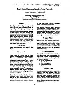
3 A BNN Classi er We adopt Mackay's BNN architecture [5]. The inputs of our BNN classi er include the values of the selected 2-gram patterns, the FASTA score, the LCC value and the score obtained from the approximately common motifs. We use one hidden layer with sigmoid activation functions, where the number of hidden units is determined experimentally. The output layer of the neural network has one output unit. The output value is bounded between 0 and 1 by the logistic activation function f (a) = 1+1e?a . The neural network is fully connected between the adjacent layers. Figure 1 illustrates the architecture of the Bayesian neural network. Let D = fx(m) ; tm g; m = 1; 2; : : : ; N; denote the training dataset, where N is the total number of training sequences in D, x(m) is an input feature vector. tm is the binary (0/1) target value for the output unit. That is, if x(m) represents a protein sequence in the globin superfamily, tm is 1; otherwise, tm is 0. Let x denote an input feature vector for a protein sequence (which could be a training sequence or a test sequence). Given the architecture A and the weights w of the BNN classi er, the output value y can be uniquely determined from the input vector x. The output value y(x; w; A) can be interpreted as P (t = 1jx; w; A), i.e., the probability that x represents a globin sequence given x; w; A. The traditional neural network suers from

2_gram_1

2_gram_n FASTA Score LCC Score LS Score

Figure 1: The Bayesian neural network architecture. the over tting problem. The weight decay is often used to avoid over tting, but there is not precise way to specify the weight decay parameter (hyperparameter), which is tuned oine. To solve this problem, the Bayesian neural network interprets the object function in the traditional neural network as the likelihood of the data given the neural network model. The weight decay term is interpreted as the prior of the neural network model. The Bayesian training of neural networks is an iterative procedure. In the implementation of the Bayesian neural network that we adopt, each iteration involves two levels of inference. At the rst level, given the value of hyperparameter that is initialized to the random value during the rst iteration, we can infer the Most Probable value of the weight vector. At the second level, the hyperparameter is optimized. The new hyperparameter value is then used in the next iteration. The process iterates a number of times. In the classi cation phase, the out-

put of a Bayesian neural network, y, is based on all models rather than one model. Each model is weighted by its posterior probability. The output of a Bayesian neural network, P (t = 1jx; D; A), is the probability that the unlabeled test sequence is a globin sequence. If it is greater than a predetermined positive threshold, the test sequence is classi ed as a globin; if it is less than a predetermined negative threshold, the test sequence is classi ed as a non-globin; otherwise the test sequence gets a \no-opinion" verdict.

4 Experiments and Results We tested our approach on two sets of data. In the rst dataset, there were 751 globin sequences (positive examples) and 293 nonglobin sequences, all selected from the PIRinternational Protein Sequence Database [1]. In the second dataset, the positive examples were the same as the rst dataset; however 736 non-globin protein sequences chosen from PROSITE [4] were used as negative examples. We used ten-fold cross validation for training and testing. The results showed that the error rate for the rst dataset was 0.3% (i.e. only 0.3% of the test sequences were misclassi ed) and the error rate for the second dataset was 0.0%. Currently we are applying our techniques to classifying DNA sequences and other types of biomolecular data.

Acknowledgment We thank Dr. David Mackay for sharing the Bayesian neural network software with us. We thank Dr. Tom Marr and Dr. Cathy Wu for providing the protein data used in the experiments. We also thank Dr. Gung-Wei Chirn for the discussion of the implementation of Sdiscovery.

References [1] W. C. Barker, J. S. Garavelli, D. H. Haft, L. T. Hunt, C. R. Marzec, B. C. Orcutt,

G. Y. Srinivasarao, L. S. L. Yeh, R. S. Ledley, H. W. Mewes, F. Pfeier, and A. Tsugita. The PIR-international protein sequence database. Nucleic Acids Research, 26(1):27{32, 1998. [2] A. Brazma, I. Jonassen, E. Ukkonen, and J. Vilo. Discovering patterns and subfamilies in biosequences. In Proceedings of the Fourth International Conference on Intelligent Systems for Molecular Biology, pp. 34{43, 1996. [3] K. A. Frenkel. The Human Genome Project and informatics. Communications of the ACM, 34(11):41{51, 1991. [4] K. Hofmann, P. Bucher, L. Falquet, and A. Bairoch. The PROSITE database, its status in 1999. Nucleic Acids Research, 27(1):215{219, 1999. [5] D. J. C. Mackay. The evidence framework applied to classi cation networks. Neural Computation, 4(5):698{714, 1992. [6] W. R. Pearson and D. J. Lipman. Improved tools for biological sequence comparison. Proceedings of the National Academy of Sciences of the USA, 85(8):2444{2448, 1988. [7] P. Petrilli. Classi cation of protein sequences by their dipeptide composition. Computer Applications in the Biosciences, 9(2):205{209, 1993. [8] G. Piatetsky-Shapiro and W. J. Frawley, editors. Knowledge Discovery in Databases, AAAI Press, Menlo Park, California, 1991. [9] J. Rissanen. Modeling by shortest data description. Automatica, 14:465{471, 1978. [10] H. C. Romesburge. Cluster Analysis for Researchers, Lifetime Learning Publications, Belmont, California, 1984. [11] C. E. Shannon. A mathematical theory of communication. Bell System Technical Journal, 27:379{423, 623{656, 1948.

[12] V. V. Solovyev and K. S. Makarova. A novel method of protein sequence classi cation based on oligopeptide frequency analysis and its application to search for functional sites and to domain localization. Computer Applications in the Biosciences, 9(1):17{24, 1993. [13] J. T. L. Wang, B. A. Shapiro, and D. Shasha, editors. Pattern Discovery in Biomolecular Data: Tools, Techniques and Applications, Oxford University Press, New York, 1999. [14] J. T. L. Wang, G. Chirn, T. G. Marr, B. A. Shapiro, D. Shasha, K. Zhang. Combinatorial pattern discovery for scienti c data: Some preliminary results. In Proceedings of the ACM SIGMOD International Conference on Management of Data, Minneapolis, Minnesota, pp. 115-125, May 1994.