Mar 9, 2010 - Neural Networks: Basic Model ... Example: Fisher's Iris Data. Modeling ... Spline. â» Generalized Additiv
Bayesian Neural Networks Yuhan Xue
March 9, 2010
Motivation
◮
Neural networks have been developed mainly by the machine learning community
◮
Statisticians often consider them to be black boxes not based on a probability model
◮
How neural networks can be applied into nonparametrics regression and classification modeling
My talk is based on Bayesian Nonparametrics via Neural Networks by Professor Herbie Lee.
Outline Bayesian Non Parametrics Model for Neural Networks BNP Regression using Local Methods BNP Regression using Basis Functions Neural Networks: Basic Model Nonparamatric Multivariate regression Nonparamatric Classification Example: Fisher’s Iris Data Modeling Issues Choosing Priors Bayesian Model Selection Conclusions
BNP Regression using Local Methods ◮
Spline
◮
Generalized Additive Model(GAM) yi =
r X
fj (xij ) + ǫi
j=1
local smoothed function for each variable without interaction effects y = f1 (x1 ) + f2 (x2 ) + ... + ǫ where fj is a one-dim spline. ◮
Prejection Persuit Regression(PPR) yi =
r X j=1
rotation of the axes
fj (β t xi ) + ǫi
BNP Regression using Basis Functions ◮
General form yi =
k X
βj fj (xi ) + ǫi
j=0
◮
Polynomial basis functions fj (x) = xj
◮
Logistic basis functions yi =
k X
�
1, x, x2 , x3 , x4 , ...
βj ψ(xi ) + ǫi , where ψ(x) =
j=0
◮
i.e.
1 1 + exp {−x}
Gaussian densities k X
� 2� xi − µj 1 x ) + ǫi , where φ(x) = √ exp − yi = βj φ( σj 2 2π j=0
Neural Networks: Basic Model yi = β0 +
k X
βj ψ(γjt xi ) + ǫi
j=1
◮
Recall Projection Persuit Regression(PPR): yi =
r X
fj (β t xi ) + ǫi
j=1
◮
Recall logistic basis functions: yi =
k X
βj ψ(xi ) + ǫi
j=0
◮
The basic neural network model = PPR + logistic basis functions
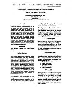
Neural Networks: Basic Model ◮
yi = β0 +
Pk
j=1 βj
Output
1 P + ǫi 1 + exp {−γj0 − rh=1 γjh xih } y
βj Hidden Nodes
3
2
1
K
γj Input
x1
x2
xr
Neural Networks: Basic Model: Example
y
Output
◮
Single input
◮
Single output
◮
2 Hidden Nodes
β2
β1
Example: Hidden Nodes
2
1 γ1
Input
γ2 x1
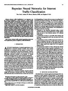
Neural Networks: Basic Model(Continued) The fitted curve: y = 4−
13.12 10.58 + 1.0 + exp(21.75 − 0.19 ∗ x) 1.0 + exp(19.60 − 0.07 ∗ x) 12 10 8 6 4 2 0 −2 −4 −6 −8
0
50
100
150
200
250
300
350
400
Neural Networks: Basic Model (Continued)
y = 4−
13.12 10.58 + 1.0 + exp(21.75 − 0.19 ∗ x) 1.0 + exp(19.60 − 0.07 ∗ x) yi = β0 +
k X
βj ψ(γjt xi ) + ǫi
j=1
◮
β0 Overall location parameter for y
◮
βj Overall scale factor for y
◮
γ0 Center of the logistic function occurs at −
◮
γ0 γ1 γj For γ1 larger, y changes at a steeper rate at the neighborhood of the center.
Outline Bayesian Non Parametrics Model for Neural Networks BNP Regression using Local Methods BNP Regression using Basis Functions Neural Networks: Basic Model Nonparamatric Multivariate regression Nonparamatric Classification Example: Fisher’s Iris Data Modeling Issues Choosing Priors Bayesian Model Selection Conclusions
Multivariate regression: Basic Setup ◮
From yig = β0g +
k X
βjg ψj (γjt xi ) + ǫig
j=1
And ψj (γjt xi ) =
1 P 1 + exp {−γj0 − rh=1 γjh xih }
The multivatiate regression model in Neural Networks: yig = β0g +
k X j=1
βjg
1 P + ǫig 1 + exp {−γj0 − rh=1 γjh xih } ǫig ∼ N (0, σ 2 )
◮
Each dimension of the output is modeled as a different linear combination of the same basis functions.
Multivariate regression: Basic Setup(Continued) ◮
From yig = β0g +
k X j=1
βjg
1 P + ǫig 1 + exp {−γj0 − rh=1 γjh xih }
Output
yp
y1
βj Hidden Nodes
3
2
1
K γj
Input
x1
x2
xr
Outline Bayesian Non Parametrics Model for Neural Networks BNP Regression using Local Methods BNP Regression using Basis Functions Neural Networks: Basic Model Nonparamatric Multivariate regression Nonparamatric Classification Example: Fisher’s Iris Data Modeling Issues Choosing Priors Bayesian Model Selection Conclusions
Classification: Basic setup An extension of multimonial likelihood approach ◮
◮
q categories {1, ..., q} ( 1, if g = yi yig = 0, otherwise Likelihood f (y|p) = ∝
n Y
i=1 n Y i=1
f (yi |pi1 , · · · , piq )
(pi1 )yi1 · · · (piq )yiq
For example, if we have three categories, then q=3 y11 = 1 y12 = 0 y13 = 0 y21 = 0 y22 = 0 y23 = 1 .. . yi1 = 0 yi2 = 1 .. .
yi3 = 0
Classification: Basic setup(Continued) ◮
exp {wig } pig = Pq g=1 exp {wig } wig = β0g +
k X
βjg ψj (γjt xi )
j=1
ψj (γjt xi ) = ◮
1 P 1 + exp {−γj0 − rh=1 γjh xih }
i = 1, ..., n Sample size h = 1, ..., r Number of imput variables j = 1, ..., k Number of hidden nodes g = 1, ..., q Number of output variables, i.e. categories ◮
Classification Rule: gˆi = argmax wig
Classification: Basic setup(Continued) ◮ ◮ ◮
exp {wig } pig = Pq g=1 exp {wig } P wig = β0g + kj=1 βjg ψj (γjt xi ) 1 P ψj (γjt xi ) = 1 + exp {−γj0 − rh=1 γjh xih } Output
y1
yp
βj Hidden Nodes
3
2
1
K γj
Input
x1
x2
xr
Classification: Fisher’s Iris Data
For simplicity, in this example I am using ◮ Classification between 2 types ◮ ◮
◮
2 input variables ◮ ◮
◮
Sepal Width Petal Width
Number of hidden nodes ◮ ◮
◮
Setosa vs. Versicolor Versicolor vs. Virginica
2 nodes 4 nodes
Maximum Likelihood
Classification: Fisher’s Iris Data Setosa vs. Versicolor Setosa vs. Versicolor
◮
2 hidden nodes
4 hidden nodes
◮
2
2
1.5
1.5 Petal Width
Petal Width
◮
1
0.5
0 2
1
0.5
2.5
3 3.5 Sepal Width
4
4.5
0 2
2.5
3 3.5 Sepal Width
4
4.5
Classification: Fisher’s Iris Data Versicolor vs. Virginica Versicolor vs. Virginica
◮
2 hidden nodes
4 hidden nodes
◮
2.5
2.5
2
2
Petal Width
Petal Width
◮
1.5
1 1
1.5
2
2.5 3 Sepal Width
3.5
4
1.5
1 1
1.5
2
2.5 3 Sepal Width
3.5
4
Outline Bayesian Non Parametrics Model for Neural Networks BNP Regression using Local Methods BNP Regression using Basis Functions Neural Networks: Basic Model Nonparamatric Multivariate regression Nonparamatric Classification Example: Fisher’s Iris Data Modeling Issues Choosing Priors Bayesian Model Selection Conclusions
Choosing Priors: Parameter Lack Interpretability Parameter may lack interpretability, so it is hard to determine a reasonable prior belief. Example: 8
8
6
6
4
4
2
2
0
0
−2
−2
−4
−4
−6
0
50
100
150
200
250
300
350
400
−6
0
50
100
150
200
250
300
350
400
Choosing Priors: Hierarchical Priors
μβ
μγ
Σβ
Σγ
γ
β
yi ∼ N
k X j=0
βj ψ(γjt xi , σ 2
βj ∼ N (µβ , σβ2 )
Σ
γj ∼ Np (µγ , Σγ ) σ 2 ∼ Γ−1 (s, S)
µβ ∼ N (aβ , Aβ )
yi
µγ ∼ N (aγ , Aγ )
σβ2 ∼ Γ−1 (cβ , Cβ ) Σγ ∼ W ish−1 (cγ , (cγ Cγ )−1 )
Choosing Priors: Comparison between Priors ◮ ◮
Problems with Improper Priors Priors in Consideration of Overfitting ◮ ◮
◮
Weight decay Shinkage Priors
Example comparing Priors
Bayesian Model Selection
Recall the Basic Model yi = β0 +
k X
βj ψ(γjt xi ) + ǫi
j=1
Bayesian model selection ◮
The covariates to be included. i.e. the optimal x
◮
The number of hidden nodes. i.e. the optimal k
◮
Modeling vs Prediction
◮
Model Averaging
Bayesian Model Selection Criteria ◮
Bayes Factors P (M1 |y) P (M1 ) P (y|M1 ) = P (M2 |y) P (M2 ) P (y|M2 )
◮
◮
BIC
ˆ Mi ) − 1 di ln n BICi = ln f (y|θ, 2
Log Scores
n
LSCV =
1X ln p(yj |y−j , Mi ) n j=1 n
LSF S = ◮
DIC
1X ln p(yj |y, Mi ) n j=1
ˆ + 2ˆ DIC(Mi |y) = D(θ) pDi
Outline Bayesian Non Parametrics Model for Neural Networks BNP Regression using Local Methods BNP Regression using Basis Functions Neural Networks: Basic Model Nonparamatric Multivariate regression Nonparamatric Classification Example: Fisher’s Iris Data Modeling Issues Choosing Priors Bayesian Model Selection Conclusions
Conclusions
Advantages ◮
Flexibility
◮
High-dimensional
◮
Good track record
Disadvantages ◮
Complexility
◮
Lack of interpretability
◮
Difficult to specify prior information