Hindawi Publishing Corporation Mathematical Problems in Engineering Volume 2016, Article ID 4280704, 15 pages http://dx.doi.org/10.1155/2016/4280704
Research Article Application of Blind Source Separation Algorithms and Ambient Vibration Testing to the Health Monitoring of Concrete Dams Lin Cheng and Fei Tong State Key Laboratory Base of Eco-Hydraulic Engineering in Arid Area, Xi’an University of Technology, Xi’an 710048, China Correspondence should be addressed to Lin Cheng;
[email protected] Received 13 August 2016; Revised 5 October 2016; Accepted 20 November 2016 Academic Editor: Yuri Vladimirovich Mikhlin Copyright © 2016 L. Cheng and F. Tong. This is an open access article distributed under the Creative Commons Attribution License, which permits unrestricted use, distribution, and reproduction in any medium, provided the original work is properly cited. In this work, using AVT data, a health monitoring method for concrete dams based on two different blind source separation (BSS) methods, that is, second-order blind identification (SOBI) and independent component analysis (ICA), is proposed. A modal identification procedure, which integrates the SOBI algorithm and modal contribution, is first adopted to extract structural modal features using AVT data. The method to calculate the modal contribution index for SOBI-based modal identification methods is studied, and the calculated modal contribution index is used to determine the system order. The selected modes are then used to calculate modal features and are analysed using ICA to extract some independent components (ICs). The square prediction error (SPE) index and its control limits are then calculated to construct a control chart for the structural dynamic features. For new AVT data of a dam in an unknown health state, the newly calculated SPE is compared with the control limits to judge whether the dam is normal. With the simulated AVT data of the numerical model for a concrete gravity dam and the measured AVT data of a practical engineering project, the performance of the dam health monitoring method proposed in this paper is validated.
1. Introduction Dam health monitoring [1] is a process based on the structural static/dynamic response and environmental variables measured by sensors installed on a dam body, foundation, and reservoir to evaluate structural health. It is an effective way to prevent the occurrence of catastrophic dam failure that would result in great loss of human life and property. Dam health monitoring is a special case of structural health monitoring (SHM) [2]. Among all SHM methods that have been proposed, the vibration-based SHM method [3] has obvious advantages. In conventional static dam health monitoring methods, the commonly measured dam responses are displacement, seepage flow, temperature, and so on, which can indicate only the local damage of a structure where the instruments are installed, and it is usually very difficult to evaluate the global state of a structure. Unlike static dam response quantities, many structural dynamic features are global, for example, changes in the natural frequencies of the structure. The advantage of global features is that damage can be detected remotely from a sensor [4]. Other dynamic
features, such as modal shape vectors, can also provide information about the damage location. Thus, using the vibrationbased method to monitor the health of large concrete dams is feasible and meaningful. Moreover, with the construction of some vibration monitoring systems, such as the dam strong earthquake monitoring system, the ambient vibration testing (AVT) [5–8] data of concrete dams under certain ambient excitation can be acquired to diagnose structural health conveniently. Therefore, research on dam health monitoring methods for concrete dams based on ambient AVT at full scale has received much attention in the last few years. To diagnose dam health using AVT data, two key steps, that is, feature extraction and feature classification, are necessary. Feature extraction is the process of identifying damage-sensitive properties, derived from the measured dynamic response, which allows one to distinguish between undamaged and damaged structures. The area of SHM that receives the most attention in the technical literature is feature extraction [9]. Although many different types of features have been reported to be used as structural damage indictors, modal features, for example, natural frequencies,
2 modal shape vectors, and coordinate modal assurance criteria (COMAC) [10], are still the most commonly used features in SHM. The advantage of using modal features is that they are independent of external ambient excitation and reflect the structural state directly. Using AVT data to identify the modal parameters of concrete dams is the operation modal analysis (OMA) [11] problem of structures. Recently, one area of research focused on OMA methods is the use of the blind source separation (BSS) technique to implement output-only modal identification. Among all proposed BSS-based OMA methods, the SOBI-based method, which has been studied in our previous work [12], shows many advantages, such as high identification accuracy, high computation efficiency, and strong robustness. The main difficulty in applying system identification for OMA of large-scale structures is the selection of the model order and the corresponding system poles. The most commonly used method is the stabilization diagram method. A conventional stabilization diagram using identified natural frequencies, damping ratios, and modal assurance criterion (MAC) is used as an index to select stable modes. Recently, a new index, modal contribution [13], has been proposed and shows better performance in discriminating structural models from mathematical poles. Whereas Cara’s work [13] shows us how to calculate the modal contribution index for the stochastic subspace identification (SSI) method [14], the procedure to calculate the modal contribution index for the SOBI-based method has not been studied. Concrete dams are large-scale engineering structures with complicated operation environments and are characterized by the structure-water interaction effect. Environmental variables, such as temperature, water level, and rainfall, cannot be ignored directly in practical engineering as in numerical and experimental investigations. Therefore, for dam health monitoring based on AVT, how to remove the variability due to environmental changes is an important problem. To monitor the health of a structure under a varying environment, a commonly used method that seeks to remove the variability due to environment without measuring the environmental variables is the latent variable-based method. For example, Sohn et al. [15], Yan et al. [16], Deraemaeker et al. [17], and Ni et al. [18] have used the principle component analysis (PCA) method for bridge structure health monitoring. In our previous work [19], the kernel component analysis (KPCA) method is adopted to monitor the health state of concrete dams. Recently, some literature has reported on the good performance of independent component analysis (ICA) [20–22], which is a typical BSS algorithm and can be deemed an extension of PCA, in state monitoring of complex systems. PCA can impose independence only up to second-order statistical information (mean and variance), whereas ICA involves higher-order statistics; that is, it not only decorrelates the data (second-order statistics) but also reduces higher-order statistical dependencies. Therefore, an ICA-based SHM method can give more sophisticated results than a PCA-based one because ICA can extract the essential independent components that drive a process. In this work, we first present a health monitoring method for concrete dams based on AVT data. Using the measured AVT data, the SOBI-based modal identification method is
Mathematical Problems in Engineering adopted to extract the basic modal parameters of a dam. For the SOBI-based modal identification method, the method to calculate the modal contribution index is proposed for the first time. The modal contribution index is then introduced into the stabilization diagram method to remove spurious modes of ambient excitation. The identified or calculated modal features are then analysed using ICA, another BSS method, to extract some ICs, which may represent the effect of environmental variables. The square prediction error (SPE) control charts and the contribution plots are then used to detect structural abnormalities and the locations of such abnormalities. At the end of this work, a numerical example and an engineering example are used to verify the proposed dam health monitoring method.
2. Modal Identification of Concrete Dams Based on SOBI and Modal Contribution 2.1. SOBI-Based Modal Identification. Based on McNeill’s derivation [23], an analytic expression of the structural acceleration response can be constructed using Hilbert transformation (HT). After considering observation noise k(𝑡), the expression of an analytic signal is as follows: C𝑎 Φ𝑅 −C𝑎 Φ𝐼 q̈ 𝑅 (𝑡) y𝑅 (𝑡) ] [ 𝐼 ] + k (𝑡) y (𝑡) = [ 𝑅 ] = [ C𝑎 Φ𝐼 C𝑎 Φ𝑅 ŷ (𝑡) q̈ (𝑡)
(1)
= Θq̈ (𝑡) + k (𝑡) , where y𝑅 (𝑡) is the physical acceleration of 𝑙 channels and ŷ𝑅 (𝑡) is its HT. The HT is performed to identify imaginary parts of modal shape vectors. C𝑎 is the acceleration response selection matrix; Φ𝑅 and Φ𝐼 are the real and imaginary parts of complex mode shapes, respectively. q̈ 𝑅 (𝑡) and q̈ 𝐼 (𝑡) are the real and imaginary parts of the modal response. If all structural modal responses are independent of each other, (1) shows a BSS problem indeed. The structural vibration response under ambient excitation can be regarded as a linear mixture of each modal response. Each modal response can then be regarded as a virtual source signal [24], and the mixing matrix is Θ. If the BSS problem can be solved, the modal parameters can be extracted from the estimated ̈ mixing matrix Θ and modal response q(𝑡). To solve the BSS problem shown in (1), the SOBI algorithm [25, 26] is adopted and a modal identification is proposed in our previous work. After the discrete sampling of the physical acceleration of 𝑙 channels at 𝑁 identical time intervals, the SOBI-based modal identification method forms a vector Y𝑘 ∈ R2𝑝𝑙×1 , which consists of the measured seismic response of 𝑙 channels y𝑘 ∈ R𝑙×1 and its time-lagged data. 𝑇
𝑇 𝑇 ⋅ ⋅ ⋅ y𝑘+𝑝−1 Y𝑘 = (y𝑘𝑇 y𝑘+1 ) , 𝑅
(𝑘 = 1, 2, . . . , 𝐿) ,
(2)
where y𝑘 = [ yŷ𝑘 ], y𝑘𝑅 is the measured physical acceleration of 𝑘 𝑙 channels at time interval k, ŷ𝑘 is its Hilbert transformation, and 𝐿 = 𝑁 − 𝑝 + 1. If 𝑙 ≥ 𝑛, then parameter 𝑝 = 1, and no time-lagged data are needed; otherwise, the time delay should
Mathematical Problems in Engineering
3
satisfy 2𝑝 × 𝑙 > 𝑛. 𝑛 is the system order, which is equal to the number of structural active modal orders multiplied by 2. The Hankel matrix H(𝜏𝑖 ) ∈ R2𝑝𝑙×2𝑝𝑙 with time delay 𝜏𝑖 can then be defined as
̃ separation matrix Θ ̃ + , and source signal, mixing matrix Θ, ̈ that is, the modal response q(𝑡), can then be expressed as ̃ = W+ U; Θ
H (𝜏𝑖 ) = 𝐸 [Y𝑘 Y𝑇𝑘+𝜏𝑖 ]
̃ + = U𝐻W; Θ
Ryy (𝜏𝑖+1 ) Ryy (𝜏𝑖 ) [ [ Ryy (𝜏𝑖+1 ) Ryy (𝜏𝑖+2 ) [ =[ [ .. .. [ . . [ [Ryy (𝜏𝑖+𝑝−1 ) Ryy (𝜏𝑖+𝑝 )
̃ + Y (𝑡) . q̈ (𝑡) = Θ
⋅ ⋅ ⋅ Ryy (𝜏𝑖+𝑝−1 )
] ⋅ ⋅ ⋅ Ryy (𝜏𝑖+𝑝 ) ] ] ], ] .. ] ⋅⋅⋅ . ] ⋅ ⋅ ⋅ Ryy (𝜏𝑖+2𝑝−2 )]
(3)
(𝜏𝑖 > 𝜏0 ) .
If 𝑙 ≥ 𝑛, 𝑝 = 1 and the Hankel matrix becomes the 𝑇 covariance function matrix Ryy (𝜏𝑖 ) = 𝐸[y𝑘 y𝑘+𝜏 ]. 𝐸[⋅] is 𝑖 the expectation operator. For a structure under white-noiselike support excitation, the covariance function matrix of the measured acceleration Ryy (𝜏𝑗 ) is related only to the initial state and system parameters (modal parameters) of the structure, which is similar to that of the structural free vibration response and the impulse response when time 𝜏𝑖 is big enough. By further deduction, the Hankel matrix H(𝜏𝑖 ) can be expressed as Θ [ ] [ ΘΣ (𝑇𝑠 ) ] [ ] ] Rq̈ q̈ (𝜏𝑖 ) H (𝜏𝑖 ) = [ .. [ ] [ ] . [ ] 𝑝−1 (𝑇 ) ΘΣ 𝑠 ] [
(6)
(4)
̃ ̈ ̈ (𝜏𝑖 ) ⋅ [Θ𝐻 Σ (𝑇𝑠 ) Θ𝐻 ⋅ ⋅ ⋅ Σ𝑝−1 (𝑇𝑠 ) Θ𝐻] = ΘR ̃q ̃ q
̃ contains the real parts Ψ𝑅 = C𝑎 Φ𝑅 The submatrix Θ of Θ and the imaginary parts Ψ𝐼 = C𝑎 Φ𝐼 of the observed complex mode shape. Using the identified real modal response q̈ 𝑅 (𝑡) and the modal identification method of the single-degreeof-freedom (SDOF) system, the natural frequencies 𝑓𝑖 (𝑖 = 1, . . . , 𝑛) and damping ratios 𝜉𝑖 (𝑖 = 1, . . . , 𝑛) can be obtained. Some details of the above modal identification method can be found in our previous work. 2.2. Modal Contribution and System Order Determination. In the modal identification process presented above, activated system order n is an important parameter. However, it is usually unknown previously. Moreover, practical ambient excitation may have some dominant frequency components and may not be like white noise support excitation at all. Therefore, it is of great importance to determine the system order and discard the dominant frequencies of ambient excitation for the OMA of concrete dams. Recently, Cara et al. proposed a new index, that is, modal contribution, to select the proper order for the state space model in the SSI method. Here, we extend this method to the SOBI-based modal identification procedure and propose an automated operation modal analysis procedure for concrete dams. 𝑅 ] ∈ R𝑙×𝑁 be the measured Let Y = [y1𝑅 , y2𝑅 , . . . , y𝑁 physical acceleration response of a dam at 𝑁 different times; Y can then be expressed as
𝐻
̃ , ⋅Θ
𝑛
where Σ(𝑇𝑠 ) = exp{Λ𝑇𝑠 }, Λ = diag(𝜆 1 , . . . , 𝜆 𝑛 ), and 𝜆 1 , . . . , 𝜆 𝑛 are the eigenvalues of the system matrix A𝑐 . Rq̈ q̈ (𝜏𝑖 ) = 𝐸[q̈ 𝑘 q̈ 𝑇𝑘+𝜏𝑖 ] = [
Rq̈ 𝑅 q̈ 𝑅 (𝜏𝑖 ) 0 0 Rq̈ 𝐼 q̈ 𝐼 (𝜏𝑖 ) ];
C𝑎 = C𝑙×𝑛 is
the output selection matrix of acceleration. Superscript 𝐻 represents Hermitian (complex conjugate and transpose). In order to realize the diagonalization of the Hankel matrix H(𝜏𝑖 ), a robust algorithm called the joint approximate diagonalization (JAD) [27] technique is adopted. Instead of diagonalizing only one Hankel matrix, a group of Hankel matrices with different time delays H(𝜏1 ), H(𝜏2 ), . . . , H(𝜏𝑠 ) are diagonalized simultaneously in the JAD technique. For the JAD technique, the corresponding optimization problem is expressed as follows: 𝑠 2 min: ∑ off (U𝐻WH (𝜏𝑖 ) W𝐻U) , 𝑖=1
(𝜏𝑖 > 𝜏0 ) .
(5)
The whitening matrix W is obtained using the PCA method. After solving the optimization problem shown above, the generalized diagonalization matrix U can be obtained. The
Y = Y𝑚 + Y𝜀 = ∑ Y𝑚𝑘 + Y𝜀 ,
(7)
𝑘=1
where Y𝑚 is the acceleration due to identified modes, Y𝑚𝑘 = 𝑚 𝑚 𝑚 [y1 𝑘 , y2 𝑘 , . . . , y𝑁𝑘 ] is the acceleration response due to the 𝑘th 𝜀 𝜀 ] is the error term of the mode, and Y = [y1𝜀 , y2𝜀 , . . . , y𝑁 measured acceleration. According to (1) and (2), the observed acceleration response y𝑘 = y𝑘𝑅 of a structure can be expressed by 𝑛
𝑛
𝑟=1
𝑟=1
𝑚
y𝑘 = ∑ [Ψ𝑅𝑟 𝑞̈ 𝑅𝑟𝑘 − Ψ𝐼𝑟 𝑞̈ 𝐼𝑟𝑘 ] + k𝑘 = ∑y𝑘 𝑟 + k𝑘 , 𝑚
(8)
where y𝑘 𝑟 is the acceleration due to the 𝑟th mode; Ψ𝑅𝑟 and Ψ𝐼𝑟 are the 𝑟th columns of matrices Ψ𝑅 and Ψ𝐼 , respectively; and 𝑞̈ 𝑅𝑟𝑘 and 𝑞̈ 𝐼𝑟𝑘 are the 𝑟th real and imaginary modal response coordinates, respectively, at the 𝑘th time interval. For the SOBI-based modal identification method mentioned in Section 2.1, Ψ𝑅𝑟 , Ψ𝐼𝑟 , q̈ 𝑅 (𝑡), and q̈ 𝐼 (𝑡) can be 𝑚 calculated using (6). The acceleration due to each mode y𝑘 𝑟 can then be calculated as shown in (8).
4
Mathematical Problems in Engineering The covariance matrix can be calculated as (Y Y𝑇 )𝐷 = (Y𝑚 Y𝑇 )𝐷 + (Y𝜀 Y𝑇 )𝐷 .
AVT data
(9) Set initial system order n = 2
The operator (⋅)𝐷 means that (M)𝐷 is a matrix consisting of the diagonal elements of matrix M and zeros elsewhere. Normalizing the above equation, 𝑛
−1
Form Hankel matrix H(𝜏i ), i = 1, 2, . . . , s
−1
(Y Y𝑇 )𝐷 (Y Y𝑇 )𝐷 = ∑ (Y Y𝑇 )𝐷 (Y𝑚𝑘 Y𝑇 )𝐷 𝑘=1
SOBI
(10)
−1
+ (Y Y𝑇 )𝐷 (Y𝜀 Y𝑇 )𝐷 . For the diagonal elements of the diagonal matrices, the following expression can be obtained:
̃ Mixing matrix 𝚯
̈ Source signal 𝒒(t)
Modal shape vectors
Damping ratios and natural frequencies
𝑛
{1}𝑚 = ∑ Δ𝑚𝑘 + Δ𝜀 ,
(11)
𝑘=1
where Δ𝑚𝑘 = diag[Δ 𝑚𝑘 (1), Δ 𝑚𝑘 (2), . . . , Δ 𝑚𝑘 (𝑙)] and Δ𝜀 = diag[Δ 𝜀 (1), Δ 𝜀 (2), . . . , Δ 𝜀 (𝑙)] are the diagonal elements of the 𝑚𝑘 𝑇 𝑇 −1 𝜀 𝑇 diagonal matrices (YY𝑇 )−1 𝐷 (Y Y )𝐷 and (YY )𝐷 (Y Y )𝐷 , respectively. The two metrics 𝛿𝑚𝑘 and 𝛿𝜀 can then be calculated using the diagonal elements of the above two matrices as 𝛿𝑚𝑘 = 𝛿𝜀 =
𝑙
1 ∑ Δ (𝑗) ; 𝑙 𝑗=1 𝑚𝑘 (12)
𝑙
1 ∑ Δ (𝑗) . 𝑙 𝑗=1 𝜀
2.3. The Flowchart of Modal Identification. After extracting the modal parameters, the MAC and COMAC could be calculated using the following equations: 𝑐 Φ𝑏𝐻 𝑗 Φ𝑗 𝑏 𝑐𝑇 𝑐 (Φ𝑏𝐻 𝑗 Φ𝑗 ) (Φ𝑗 Φ𝑗 )
,
(13) (𝑗 = 1, 2, . . . , 𝑛) ,
COMAC (𝑘) =
2 ∑𝑛𝑗=1 Φ𝑏𝑗𝑘 ⋅ Φ𝑐𝑗𝑘 2
∑𝑛𝑗=1 Φ𝑏𝑗𝑘 ∑𝑛𝑟=1 Φ𝑐𝑗𝑘 2
Yes
n < nmax No Plot stabilization diagram and 𝛿m𝑘 ∼n curve
Select stable modes
Figure 1: Modal identification procedure based on SOBI and modal contribution using AVT data.
As noted by Cara et al., 𝛿𝑚𝑘 indicates the importance of the 𝑘th identified mode; the modal contributions of these spurious modes and weak modes are almost zero. In the vector 𝛿𝑚 = (𝛿𝑚1 , 𝛿𝑚2 , . . . , 𝛿𝑚𝑛 ), the greater the number of nonzero elements is, the more the activated modes are included in the vibration response and the more abundant the information therein is.
MAC (𝑗) =
Modal contribution metrics 𝛿m𝑘
n=n+2
,
(14) (𝑘 = 1, 2, . . . , 𝑙) ,
where Φ𝑏𝑗 is the 𝑗th modal shape vector of an undamaged structure; Φ𝑐𝑗 is the 𝑗th modal shape vector of a structure with
an unknown state; and Φ𝑏𝑟𝑘 and Φ𝑐𝑟𝑘 are the 𝑘th components of modal shape vectors Φ𝑏𝑟 and Φc𝑟 , respectively.
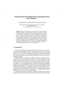
Many researchers have proved that MAC and COMAC are more sensitive to structural damage than natural frequencies and modal shape vectors. In addition, COMAC can also provide damage location information of a structure. According to the SOBI-based modal identification methods, stabilization diagram, and proposed modal contribution index, an OMA procedure for concrete dams using AVT data is proposed. The flowchart of the integrated OMA method is shown in Figure 1.
3. Dam Health Monitoring Using an ICA-Based Method The preceding section described a procedure to obtain an 𝑛dimensional feature space of modal features. In a situation where multidimensional feature vectors exist, several monitoring methods may be employed for feature vector discrimination [28]. As a result of environmental variables and some other stochastic factors, the 𝑛-dimensional feature vector is random. For a multidimensional random variable, the statistical process control- (SPC-) based method can be adopted to evaluate the structural health based on identified modal features. SPC is a collection of tools useful in process monitoring. The control chart is the most commonly used one and is very suitable for automated continuous system monitoring.
Mathematical Problems in Engineering
5
Hereafter, a newly developed ICA-based SPC method is introduced into the dam health monitoring process. 3.1. Perform ICA on the Extracted Modal Features. Assume that the identified modal features (natural frequencies, modal shape vectors, MAC or COMAC, etc.) are arranged in a zeromean vector x(𝑡) with 𝑚 components, 𝑥1 , 𝑥2 , . . . , 𝑥𝑚 , which can be expressed as [1, 16] x (𝑡) = f (𝐻, 𝑇, 𝜃, . . .) + g (𝜂) = x̃ (𝑡) + 𝜀 (𝑡) ,
(15)
where f(⋅) is a vector nonlinear function that projects environmental variables, such as water level 𝐻, temperature 𝑇, and time effect 𝜃, into the determined components x̃(𝑡) of structural dynamic features. For a concrete dam without damage, x̃(𝑡) preserves the major information of the calculated modal features x(𝑡), which is mainly the effect of some environmental variables; 𝜀(𝑡) = 𝑔(𝜂) is the random component, which contains the influence of some other random factors 𝜂, such as the identification error of modal features. The nonlinear mapping f(⋅) is expressed as another nonlinear mapping Θ(⋅) multiplied by a linear mapping Λ, that is, x̃ (𝑡) = f (𝐻, 𝑇, 𝜃, . . .) = Λ [Θ (𝐻, 𝑇, 𝜃, . . .)] = Λ𝜉 (𝑡) , (16) where 𝜉(𝑡) = [𝜉1 , . . . , 𝜉𝑠 ]𝑇 is called the latent variables vector. Latent variables 𝜉1 , . . . , 𝜉𝑠 are independent of each other. The number of latent variables 𝑠 ≤ 𝑚. For a concrete dam that has worked a long time or has recently undergone a large earthquake or flood, some damage may be found, and the damage will change the probability distribution of random vector 𝜀(𝑡). Therefore, the structural damage can be detected by comparison of the probability distribution of 𝜀(𝑡) after the determined components have been extracted. Hereafter, the ICA-based method is adopted to identify the linear mapping matrix Λ and the latent variables 𝜉1 , . . . , 𝜉𝑠 , also called independent components (ICs), to calculate the two parts, that is, x̃(𝑡) and 𝜀(𝑡). The principle of ICA estimation is based on the central limit theorem (CLT), which states that the sum of independent random variables tends to be distributed towards Gaussian, regardless of the underlying distribution. This means that a mixture of some independent random variables is always Gaussian for the original variables. Usually, in ICA, the original feature samples must be whitened first. The whitened variables z(𝑡) are obtained by z (𝑡) = Qx (𝑡) = QΛ𝜉 (𝑡) + Q𝜀 (𝑡) ,
(17)
where the whitening matrix Q = diag(𝜆 1 , 𝜆 2 , . . . , 𝜆 𝑚 )−1/2 [𝛽1 , 𝛽2 , . . . , 𝛽𝑚 ]𝑇 is obtained using PCA. 𝜆 𝑖 , 𝑖 = 1, . . . , 𝑚, are eigenvalues of the covariance matrix C𝑥 = 𝐸(xx𝑇 ); 𝛽𝑖 , 𝑖 = 1, . . . , 𝑚, are its eigenvectors. The goal of ICA is to find a de-mixing matrix W = O𝑇 Q from the original observed data x(𝑡) such that the estimated ICs, that is, latent variables, can be expressed as 𝜉̃ (𝑡) = Wx (𝑡) = O𝑇 z (𝑡) ,
(18)
where O is an orthonormal matrix and determined by maxĩ mizing the non-Gaussianity of 𝜉(𝑡). The non-Gaussianity of a random variable 𝜐 can be measured by negentropy. The negentropy can be approximated by the kurtosis kurt(𝜐) 2
kurt (𝜐) = 𝐸 [𝜐4 ] − 3 (𝐸 [𝜐2 ]) .
(19)
For a Gaussian random variable 𝜐, negentropy equals zero, and kurt(𝜐) = 0. With increasing non-Gaussianity of a random variable, negentropy increases. Therefore, the basic principle of the ICA estimation method can be summarized as finding the proper demixing matrix W, which can maximize the non-Gaussianity measured by the negentropy of each recovered IC. Another measure of the non-Gaussianity of a random variable is the entropy-based negentropy, which is more statistically justified. The entropy of a discrete random variable can be calculated as 𝐻 (𝜐) = −∑𝑝 (𝜐 = 𝜐𝑖 ) ⋅ log 𝑝 (𝜐 = 𝜐𝑖 ) , 𝑖
(20)
where 𝑝(⋅) is the discrete probability distribution function. The Gaussian random variable has the largest entropy among all other random variables with equal variance; that is, it is the most random or uncertain one. For a random variable with less Gaussianity, the definition of negentropy is given as follows: 𝐽 (𝜐) = 𝐻 (𝜐gau ) − 𝐻 (𝜐) ,
(21)
where 𝜐gau is a standard Gaussian random variable with zero mean and unit variance. The proper demixing matrix W = O𝑇 Q is obtained through an optimization process which maximizes the nonGaussianity of each latent variable and the non-Gaussianity is measured by negentropy calculated using (21). In order to realize this optimization object, the most widely used algorithm, that is, the FastICA algorithm [29], is adopted in this study. Then the ICs called latent variables for the process monitoring problem can be calculated using (18). In the error space, the square prediction error (SPE) can be calculated for use as an index of structural health. SPE (𝑡) = [x (𝑡) − Q−1 O𝑇𝑑 O𝑑 Ox (𝑡)]
𝑇
⋅ [x (𝑡) − Q−1 O𝑇𝑑 O𝑑 Qx (𝑡)] ,
(22)
where O𝑑 is composed of the first 𝑑 row vectors of O. Selecting an appropriate parameter 𝑑 is a key step of the above procedure. This parameter determines the division of the observation space into the dominant components space and the residual parts space. Based on Wang’s proof, ICs could be ranked and selected by the value of the 𝐿 2 norm of a mixing matrix Λ column according to the minimum mean square error (MSE). The criterion can be expressed as 𝑑
̃ = arg max∑ a 2 , arg min 𝐽 (𝜉) 𝑖 𝜉𝑖
𝜉𝑖 𝑖=1
where a𝑖 is the 𝑖th column of mixing matrix Λ.
(23)
6
Mathematical Problems in Engineering
3.2. Setting Control Limits for SPE. When the majority of nonGaussianity is removed by the ICs, the noise in the residuals 𝜀(𝑡) will approximately follow a Gaussian distribution, so the control limit of SPE can be calculated from the following weighted 𝜒2 distribution: SPE ∼ 𝜇𝜒2 .
(24)
In addition, the kernel density estimation (KDE) method proposed by Martin and Morris [30] can also be used to determine the confidence limit of the SPE statistic because it does not require an assumption for the distribution of data. ̃ Using the KDE-based method, the probability function 𝐷(𝜐) of the SPE index can be evaluated by 𝑛 ̃ (𝜐) = 1 ∑𝜅 ( 𝜐 − 𝜐𝑖 ) , 𝐷 𝑁𝑠 ℎ 𝑖=1 ℎ
(25)
where commonly used kernel function 𝜅(⋅) is a Gaussian function, 𝑁𝑠 is the sample number, ℎ is the time window length, and 𝜐𝑖 is the 𝑖th monitoring data point. Given a testing level 𝛼, the upper control limit (UCL) can be determined using the estimated probability function as follows: 𝑃 (𝜐 < UCL) = 1 − 𝛼.
Step 2. With these preprocessed AVT data, some basic modal parameters of structure are identified using the proposed modal identification procedure shown in Figure 1. Then, using (14), the COMAC index is calculated. For each type of modal feature, construct a data matrix X = [x1 , . . . , x𝑁], which includes the reference data for dam health monitoring. Step 3. After normalizing these data of the modal features by their mean 𝜇 and variance 𝜎, the ICA is adopted to analyse the normalized multidimensional time series x1 , . . . , x𝑁 to extract some ICs. The determined component is x̃(𝑡), and noise residuals are 𝜀(𝑡). The SPE metrics are calculated using (22). Given a testing level 𝛼, (26) determines the UCL of SPE for a dam without damage. Step 4. For each newly obtained AVT data, the above mentioned Steps 1∼3 are repeated and the SPE index is calculated. These newly calculated SPE indices are compared with the UCL calculated using (26) to determine whether the structure is normal. If the new SPE metrics exceed the control limit, the dam is abnormal; otherwise, it is still in the normal state.
(26)
The UCL is calculated to determine whether the SPE index is normal. When the calculated SPE index is greater than the UCL, the structure may be abnormal. If the analysed features are modal shapes, COMAC, and other metrics that can provide information on the damage location, the distribution of SPE index for different sensors indicates the location of structural damage. Then, another analysis tool called contribution plots [31] is used to locate the position of sensors with abnormal information. The SPE shown in (22) can be rewritten in the following expression: 𝑙 𝑙 2 ̃𝑗 = ∑ Cspe , SPE = ∑ X𝑗 − X 𝑗 𝑗=1 𝑗=1
Therefore, some preprocessing procedures are necessary to be adopted to improve the signal-to-noise ratio (SNR) of the AVT data.
(27)
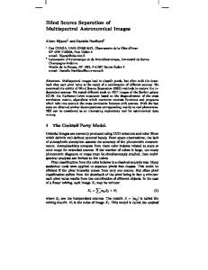
̃𝑗 are the identified and the reconstructed where X𝑗 and X modal features (natural frequencies, modal shape vectors, or COMAC) of the 𝑗th mode, respectively. The reconstructed modal features are obtained by ICA. Cspe𝑗 is the contribution of component 𝑗 of the vibration characteristic to the SPE norm. 3.3. The Flowchart of ICA-Based Dam Health Monitoring. Now, a detailed step-by-step description of the dam health monitoring method based on AVT and two different BSS methods will be given in the following. The flow chart of this dam health monitoring method is shown in Figure 2. Step 1. Through the vibration measurement system of a concrete dam, the AVT data can be obtained at different times, when the structure can be deemed as normal. The original AVT data may include the disturbance of measurement noise.
Step 5. When the calculated SPE index is greater than the UCL and the structure is deemed as abnormal, the SPE contribution plots and the local modal features are used to locate the structural damage. Local features are those modal features which can provide damage location information. If some obvious peaks appeared on the SPE contribution plots around some sensors number, damage may occur around these sensors.
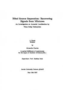
4. Case Study 4.1. Numerical Verification. Before analysing practical AVT data, the simulated AVT data using FEM are used to validate the proposed dam health monitoring method. The 3D finite element model of the maximum dam block of a concrete gravity dam is constructed as shown in Figure 3. The locations of 10 acceleration sensors with three measurement directions and a simulated crack are shown in Figure 3(a). The width of the dam block is 10 m. The dynamic elastic modulus, Poisson’s ratio, and mass density of dam concrete are 31.0 GPa, 0.2, and 2643 kg/m3 , respectively; the dynamic elastic modulus and Poisson’s ratio of foundation rock are 20.0 GPa and 0.25, respectively. A massless foundation is used to model the dam-foundation interaction when calculating the vibration response of a structure. The ambient excitation used in each FEM calculation is a white noise time series, which is generated using the MATLAB program. The AVT data are obtained by adding the calculation results of the FEM software MSC.Marc [32] using the mode-superposition method (10 modes are used) with some noise. The simulated AVT record of sensor #1 in 3 measurement channels is shown in Figure 4. The sampling frequency of the simulated acceleration measurement is 100 Hz and the total number of sample is 1000.
Mathematical Problems in Engineering
7
Dam
Dam
Healthy
?
Referenced AVT data
New AVT data
Modal features
Modal features Mean 𝜇 and variance 𝜎
Normalized data
Normalized data De-mixing
ICA
matrix W ICs
Calculate SPE Calculate SPE Determine upper control limit UCL
UCL
Contribution plots
Location of damage
Yes
Local features
Global features
SPE > UCL?
SPE > UCL?
No
Yes
Abnormal
No Normal
Figure 2: The dam health monitoring method based on AVT and ICA. 14.8 m
36.5 m
#2
#1
#4
#3 Crack zone
Reservoir water Dam
#6
5#
#8
#7
#9
70.0 m (a)
66.5 m
19.25 m
Foundation rock
#10 (b)
Figure 3: (a) Model size, a simulated crack and the location of acceleration sensors; (b) the finite element model of the dam-reservoirfoundation system.
8
Mathematical Problems in Engineering Table 1: A comparison of the calculated and identified no-damping natural frequencies (unit: Hz).
Method FEM SSI SOBI
1 1.05 1.06 1.06
2 2.51 2.50 2.51
3 3.77 3.78 3.77
4 5.56 5.57 5.57
5 6.25 6.24 6.24
6 7.91 7.85 7.93
7 8.34 8.35 8.35
8 10.91 10.91 10.91
9 11.93 11.92 11.93
10 12.53 12.53 12.54
Table 2: The false alarm rate and missing alarm rate of the dam health monitoring. Case
Alarm rate 𝑃𝐹 𝑃𝐶 𝑃𝐹 𝑃𝐶 𝑃𝐹 𝑃𝐶 𝑃𝐹 𝑃𝐶 𝑃𝐹 𝑃𝐶
1 2 3 4 5
PCA Frequency 2.5% 97.5% 2.0% 98.0% 57.5% 42.5% 34.0% 66.0% 11.0% 89.0%
KPCA COMAC 0.5% 99.5% 0.0% 100.0% 7.5% 92.5% 0.0% 100.0% 0.0% 100.0%
Acceleration (cm/s2 ) Acceleration (cm/s2 )
2000 1000 0 −1000 −2000
Acceleration (cm/s2 )
Channel 1 3000 1000 −1000 −3000
2000 1000 0 −1000 −2000
0
100 200 300 400 500 600 700 800 900 1000 Sample number Channel 2
0
100 200 300 400 500 600 700 800 900 1000 Sample number Channel 3
0
100 200 300 400 500 600 700 800 900 1000 Sample number
Figure 4: Simulated AVT data of sensor #1 in 3 measurement channels.
To validate the modal identification procedure based on SOBI and modal contribution, the simulated AVT data are used to extract structural modal parameters using SOBI and SSI. The practical modal parameters of the dam are calculated using FEM. The identified and calculated no-damping natural frequencies are shown in Table 1. As shown in Table 1, the maximum relative errors of the modal identification results for the SOBI and SSI methods are 0.95% and 1.03%, respectively. Setting 𝑛max = 50, the modal contribution index and singular value spectrum are shown in Figure 5. As shown in Figure 5(a), when the system order is higher than 20, the modal contribution index tends to become a stable constant, whereas in the singular value spectrum, no obvious drop is observed. The increase in noise level will increase the modal
Frequency 0.0% 100.0% 1.5% 98.5% 7.5% 92.5% 15.5% 84.5% 5.0% 9.5%
ICA COMAC 0.0% 100.0% 0.0% 100.0% 5.0% 95.0% 0.0% 100.0% 0.0% 100.0%
Frequency 0.0% 100.0% 2.0% 98.0% 6.0% 94.0% 7.0% 93.0% 0.0% 100.0%
COMAC 0.50% 99.50% 0.0% 100.0% 2.5% 97.5% 0.0% 100.0% 0.0% 100.0%
contribution index, but the position of the turning point will not be changed. The modal contribution of 10 activated modes is shown in Figure 5(c). The relationship between the identified first- and secondmode natural frequencies and the water level is shown in Figure 6. Because the reservoir water will provide additional mass to the dam-foundation-reservoir system, Figure 6 shows that the natural frequencies decrease with increasing water level. In this numerical example, to evaluate the impact of environmental variables (here, only the water level is simulated) and damage extent on the identification results of vibration features, five simulation cases are designed. The crack lengths corresponding to the five cases are 0 m, 0 m, 2 m, 4 m, and 6 m. For each of the five cases, 200 different water levels are selected randomly within the water level range [75 90] m, and then, the acceleration responses measured by sensors numbered #1∼#10 are calculated using the FEM. Case number 1 is designed to generate referenced data, and case number 2 is used to verify the false alarm rate of the proposed method. For the simulated AVT data of case number 1 and case number 5, the identified modal natural frequencies of the 1st mode and the 10th mode are shown in Figure 7. As shown in this figure, the effect of damage cannot be distinguished directly as a result of the variation in water level. Using the modal features, that is, the natural frequencies and COMAC, PCA, KPCA, and ICA are adopted to monitor the dam health. A comparison of the false alarm rate and missing alarm rate of the three analysis methods is shown in Table 2. For the PCA and ICA method, the SPE index and UCL are shown in Figure 8. The false alarm rate 𝑃𝐹 and correct alarm rate 𝑃𝐶 can be defined as 𝑁 𝑃𝐹 = 𝐹 × 100%; 𝑁 (28) 𝑃𝐶 = 1 − 𝑃𝐹 ,
Mathematical Problems in Engineering
9
1.1
2
1
1
0.9 log(𝜎)
𝛿m
0.8 0.7 0.6 0.5
0 −1 −2
0.4 0
5
10
15
20 25 System order
30
35
−3
40
0
SNR = 30 db SNR = 20 db
No noise SNR = 50 db SNR = 40 db
5
10
15
20 25 System order
30
35
40
SNR = 30 db SNR = 20 db
No noise SNR = 50 db SNR = 40 db
(a)
(b)
0.5 0.4
𝛿m𝑘
0.3 0.2 0.1 0
0
5
10
15
20 25 30 Frequency (Hz)
35
40
45
50
(c)
Figure 5: (a) Modal contribution plots; (b) singular value plots; (c) modal contribution of different modes. 2.8
1.14
Natural frequency (Hz)
Natural frequency (Hz)
1.16 1.12 1.1 1.08 1.06 1.04 1.02 1 75
80
85
90
95
Water depth (m) (a)
2.7 2.6 2.5 2.4 2.3 75
80
85
90
95
Water depth (m) (b)
Figure 6: The relationship between natural frequencies and water level for (a) the first mode and (b) the second mode.
where, 𝑁 is the total number of modal features and 𝑁𝐹 is the number of false alarming. It can be seen in Table 2 and Figure 9 that the ICA-based dam health monitoring method has higher alarm accuracy than the other two methods, especially for a dam with a small damage extent. For the simulated case 4, the contribution plots of SPE are shown in Figure 10. As shown in this figure, an obvious peak of SPE can be found near sensor #5, which is just the location where the crack is simulated. In practical engineering application, acceleration sensors may be not just installed near a crack zone, since the location
of crack is commonly unknown in advance. In order to verify the performance of the proposed ICA-based SHM method when sensors are far away from structural damage zone, the acceleration sensors are rearranged, as is shown in Figure 11. For the new arrangement of sensors, the dam health monitoring results using COMAC index and ICA-based method are shown in Figure 12. The SPE control chart shows the damage can be detected effectively. The contribution plots show two peaks at the sensor numbered #5 and #6, but the two peaks are not very obvious since the distance between the two sensors and crack zone is little far (4.5 m indeed).
1.16 1.12 1.08 1.04 1
0
20
40
60
80
100
120
140
160
180 200
Natural frequency (Hz)
Mathematical Problems in Engineering
Natural frequency (Hz)
10
14 13.5 13 12.5 12 11.5
0
20
40
60
80
Sample number
100
120
140
160
180 200
Sample number
Case 1 Case 5
Case 1 Case 5 (a)
(b)
25 20 15 10 5 0
Case 1
Case 2
Case 3
Case 4
Case 5
UCL, 𝛼 = 0.01
0
100
200
SPE
SPE
Figure 7: A comparison of identified natural frequencies of case 1 and case 5 for (a) the first mode and (b) the tenth mode.
300
400 500 600 700 Sample number
800
900 1000
60 50 40 30 20 10 0
Case 1
Case 2
Case 3
Case 4
Case 5
UCL, 𝛼 = 0.01
0
100
200
300
400 500 600 700 Sample number
(a)
800
900 1000
(b)
4 3 2 1 0
Case 1
Case 2
Case 3
Case 4
Case 5 SPE
SPE
Figure 8: Dam health monitoring results using natural frequencies for the (a) PCA-based method and (b) ICA-based method.
UCL, 𝛼 = 0.01
0
100
200
300
400 500 600 700 Sample number
800
900 1000
Case 1 Case 2 Case 3 Case 4 Case 5 30 25 20 15 10 UCL, 𝛼 = 0.01 5 0 0 100 200 300 400 500 600 700 800 900 1000 Sample number
(a)
(b)
Figure 9: Dam health monitoring results using COMAC index for the (a) PCA-based method and (b) ICA-based method.
10
7
3
6 5
#3
32.0 m
4 #4
2
4 3
1
2 20
40
60
#5 Crack zone #6
#7
4.5 m 4.5 m
19.25 m
80 100 120 140 160 180 200 Sample number
Figure 10: Contribution plot of SPE for case 4.
4.2. Analysing the Practically Measured AVT Data. A hydropower station is located in the middle stream of the Minjiang River in Fujian Province of China. The maximum height of the roller-compacted concrete (RCC) gravity dam is 101.0 m, and its normal flood level elevation is 65.0 m, with a corresponding storage capacity of 2.6 × 10⁹ m3 . This project
#9
#8
#10 70.0 m
62.0 m
Sensor number
#2
#1
8
1
14.8 m
5
9
#11
Figure 11: New arrangement of acceleration sensors.
Mathematical Problems in Engineering
11 15
SPE
35 30 25 20 15 10 5 0
Case 1
Case 2
Case 3
Case 4
Cspe
10 Case 5
5 UCL, 𝛼 = 0.01
0
100
200
300
400 500 600 700 Sample number
n n 800 1 900 2 1000
0
1
2
3
4
5 6 7 8 Sensor number
(a)
9
10
11
(b)
12 10
Cspe
8 6 4 2 0
1
2
3
4
5 6 7 8 Sensor number
9
10
11
(c)
Figure 12: Dam health monitoring results using COMAC index for the ICA-based method, (a) SPE control chart and (b) contribution plots at the sample number 𝑛1 and (c) at the sample number 𝑛2 of case 5.
Monitoring center
SE5
74.00 Dam crest
19
20
SE1
SE7
2 22
SE6
19
SE3 25
Vertical direction
SE2
32.00 26
74.00
18
Dam base
53.00 Pier bottom
11.30
Monitoring house
Dam crest
SE1
32.00
24
Vertical direction
Gallery −4.80 −11.50
SE4 Gallery
−26.00
−19.00
River flow direction
Dam axis direction Accelerometer
(a)
SE2
Dam axis direction
River flow direction Accelerometer
Gallery 11.30 SE3 Gallery −11.50
SE4
(b)
Figure 13: Arrangement of seismographs on the RCC dam.
is located near the Taiwan Strait seismic zone, so seismographs are installed on the 19th and 25th dam blocks. The arrangement and location of these seismographs are shown in Figure 13. Because each dam monolith in the concrete gravity dam works independently, in this study, only the vibration response record of dam monolith number 19 is studied. The ambient vibration response record of 56 different measurement times is used. The sample size of each AVT record is 16,000, and the sampling frequency is 100 Hz. The AVT data of all nine channels measured on August 19, 2003 are shown in Figure 14. Using the AVT data of 56 different measurement times, the modal parameters are identified based on the proposed
automated modal identification procedure. Seven modes with larger modal contributions than the other modes are used to monitor the dam health, and their identification results are shown in Figure 15(a). The modal contribution of the seven modes is shown in Figure 15(b). The identified natural frequencies (7 orders) and calculated COMAC index using the AVT data of the dam for the first 40 times are used as reference data. For the other 16 measurement times, the structural health is diagnosed using the PCA, KPCA, and ICA methods. The dam health diagnosis result based on these data is shown in Figures 16 and 17. UCL is calculated by setting the test level 𝛼 = 0.01 using (26). From the two figures, we can see that the health state of the
2000
4000
6000 8000 10000 12000 14000 16000 Sample number
Seismograph SE1, channel 3, river flow direction
0
2000
4000
6000 8000 10000 12000 14000 16000 Sample number
Seismograph SE2, channel 5, river flow direction 2000 1000 0 −1000 −2000 0
2000
4000
6000 8000 10000 12000 14000 16000 Sample number
Seismograph SE4, channel 7, vertical direction
1000 500 0 −500 −1000
0
2000
4000
6000 8000 10000 12000 14000 16000 Sample number 1500 1000 500 0 −500 −1000 −1500
Acceleration (10−6 g)
0
3000 2000 1000 0 −1000 −2000 −3000
Acceleration (10−6 m/s2 )
6000 4000 2000 0 −2000 −4000 −6000
Seismograph SE1, channel 1, vertical direction
1500 1000 500 0 −500 −1000 −1500
Acceleration (10−6 g)
4000 3000 2000 1000 0 −1000 −2000 −3000
1500 1000 500 0 −500 −1000 −1500
Acceleration (10−6 g)
Mathematical Problems in Engineering
Acceleration (10−6 g)
Acceleration (10−6 g)
Acceleration (10−6 g)
Acceleration (10−6 g)
Acceleration (10−6 g)
12
1000
Seismograph SE1, channel 2, dam axis direction
0
2000
4000
6000 8000 10000 12000 14000 16000 Sample number
Seismograph SE2, channel 4, dam axis direction
0
2000
4000
6000 8000 10000 12000 14000 16000 Sample number
Seismograph SE3, channel 6, river flow direction
0
2000
4000
6000 8000 10000 12000 14000 16000 Sample number
Seismograph SE4, channel 8, dam axis direction
500 0 −500 −1000
0
2000
4000
6000 8000 10000 12000 14000 16000 Sample number
Seismograph SE4, channel 9, river flow direction
0
2000
4000
6000 8000 10000 12000 14000 16000 Sample number
Figure 14: The AVT data of the dam monolith number 19 measured on August 19, 2003.
dam is normal at the 16 different times, which is consistent with the diagnosis result using the static monitoring data of displacement and flow seepage.
5. Conclusions The dam health monitoring method presented in this work includes a modal identification procedure based on SOBI and modal contribution index and a SPC method based on ICA. The modal contribution index calculation method for
SOBI-based modal identification is studied to determine the system orders. ICA and SPE contribution plots are used for the calculated modal features to detect structural damage and determine the location of it. The numerical example and the engineering example have verified the good performance of these proposed methods. The advantages of the vibrationbased structural health monitoring method have been widely applied in many fields of civil engineering. For dam and some other concrete hydraulic structures, since much more attentions have been paid to the construction of vibration
Mathematical Problems in Engineering
13
0.25 0.2
50 40 30 20 10 0
𝛿m𝑘
Natural frequency (Hz)
0.15 0.1 0.05 0 0
4
8
12 16 20 24 28 32 36 40 44 48 52 56 Measurement number
0
5
10
(a)
15
20 25 30 Frequency (Hz)
35
40
45
(b)
Figure 15: (a) Identification results of natural frequencies using the AVT data of 56 different times and (b) modal contribution index for each identified mode.
Referenced data using PCA
3
2.5
2.5 UCL, 𝛼 = 0.01
1.5
1
0.5
0.5 5
10
15 20 25 Sample number
30
35
SPE
0.05
4
6 8 10 Sample number
12
14
16
12
14
16
12
14
16
Compared data using KPCA
UCL, 𝛼 = 0.01
0.1 0.05
0
5
10
15 20 25 Sample number
30
35
0
40
Referenced data using ICA
6
0
2
4
UCL, 𝛼 = 0.01
5
4
6 8 10 Sample number Compared data using ICA
6
UCL, 𝛼 = 0.01
5
4 SPE
SPE
2
0.15
0.1
3
3
2
2
1
1
0
0
0.2
UCL, 𝛼 = 0.01
0.15
0
0
40
Referenced data using KPCA
0.2
SPE
1.5
1
0
UCL, 𝛼 = 0.01
2 SPE
SPE
2
0
Compared data using PCA
3
0
5
10
15 20 25 Sample number
30
35
40
0
0
2
4
6 8 10 Sample number
Figure 16: Dam health monitoring using the PCA, KPCA, and ICA methods for the referenced data and compared data of natural frequencies.
14
Mathematical Problems in Engineering Referenced data using PCA
2
1 0.5
0
5
10
15 20 25 Sample number
35
0
40
UCL, 𝛼 = 0.01
0
5
10
15 20 25 Sample number
30
35
40
Referenced data using ICA
1.5
1.2 1.1 1 0.9 0.8 0.7 0.6 0.5 0.4 0.3 0.2
0
2
4
1
12
14
16
12
14
16
12
14
16
UCL, 𝛼 = 0.01
0
2
4
6 8 10 Sample number Compared data using ICA
1.5
UCL, 𝛼 = 0.01
6 8 10 Sample number
Compared data using KPCA
2
SPE
SPE
30
Referenced data using KPCA
2
UCL, 𝛼 = 0.01
1 0.5
0.5 0
1 0.5
SPE
SPE
1.2 1.1 1 0.9 0.8 0.7 0.6 0.5 0.4 0.3 0.2 0.1 0
UCL, 𝛼 = 0.01
1.5 SPE
SPE
1.5
0
Compared data using PCA
2
UCL, 𝛼 = 0.01
0
5
10
15 20 25 Sample number
30
35
40
0
0
2
4
6 8 10 Sample number
Figure 17: Dam health monitoring using the PCA, KPCA, and ICA method for the referenced data and compared data of COMAC index.
monitoring systems, the dam health monitoring method proposed in this work is expected to be widely applied in realistic engineering.
Competing Interests The authors declare that they have no competing interests.
Acknowledgments This work was supported by the National Natural Science Foundation of China (Grants nos. 51409205, 51279052, 51409018, and 51309189), Project Funded by China Postdoctoral Science Foundation (Grant no. 2015M572656XB) and Postdoctoral Science Foundation of Shanxi Province, Open Foundation of State Key Laboratory of Hydrology-Water Resources and Hydraulic Engineering (Grant no. 2014491011), the Program 2013KCT-15 for Shanxi Provincial Innovative
Research Team, and the Innovative Research Team of Institute of Water Resources and Hydroelectric Engineering, Xi’an University of Technology (Grant no. 2016ZZKT-14).
References [1] L. Cheng and D. Zheng, “Two online dam safety monitoring models based on the process of extracting environmental effect,” Advances in Engineering Software, vol. 57, pp. 48–56, 2013. [2] H. Sohn, C. R. Farrar, F. M. Hemez et al., A Review of Structural Health Monitoring Literature: 1996–2001, Los Alamos National Laboratory, New Mexico, NM, USA, 2003. [3] S. W. Doebling, C. R. Farrar, and M. B. Prime, Damage Identification and Health Monitoring of Structural and Mechanical Systems from Changes in their Vibration Characteristics, a Literature Review, Los Alamos National Laboratory, Los Alamos, NM, USA, 1996. [4] J. Zhao and J. T. DeWolf, “Sensitivity study for vibrational parameters used in damage detection,” Journal of Structural Engineering, vol. 125, no. 4, pp. 410–416, 1999.
Mathematical Problems in Engineering [5] B. Sevim, S. Atamturktur, A. C. Altunis¸ik, and A. Bayraktar, “Ambient vibration testing and seismic behavior of historical arch bridges under near and far fault ground motions,” Bulletin of Earthquake Engineering, vol. 14, no. 1, pp. 241–259, 2016. [6] B. Sevim, A. C. Altunis¸ik, and A. Bayraktar, “Earthquake behavior of berke arch dam using ambient vibration test results,” Journal of Performance of Constructed Facilities, vol. 26, no. 6, pp. 780–792, 2012. [7] G. R. Darbre, C. A. M. De Smet, and C. Kraemer, “Natural frequencies measured from ambient vibration response of the arch dam of Mauvoisin,” Earthquake Engineering and Structural Dynamics, vol. 29, no. 5, pp. 577–586, 2000. [8] C.-H. Loh and T.-S. Wu, “Identification of Fei-Tsui arch dam from both ambient and seismic response data,” Soil Dynamics and Earthquake Engineering, vol. 15, no. 7, pp. 465–483, 1996. [9] E. P. Carden and P. Fanning, “Vibration based condition monitoring: a review,” Structural Health Monitoring, vol. 3, no. 4, pp. 355–377, 2004. [10] N. A. J. Lieven and D. J. Ewins, “Spatial correlation of mode shapes the coordinate modal assurance criterion,” in Proceedings of the 6th International Modal Analysis Conference, vol. 3, pp. 690–695, 1988. [11] C. Rainieri and G. Fabbrocino, Operational Modal Analysis of Civil Engineering Structures, Springer, Berlin, Germany, 2014. [12] L. Cheng and D. Zheng, “The identification of a dam’s modal parameters under random support excitation based on the Hankel matrix joint approximate diagonalization technique,” Mechanical Systems and Signal Processing, vol. 42, no. 1-2, pp. 42–57, 2014. [13] F. J. Cara, J. Juan, E. Alarc´on, E. Reynders, and G. De Roeck, “Modal contribution and state space order selection in operational modal analysis,” Mechanical Systems and Signal Processing, vol. 38, no. 2, pp. 276–298, 2013. [14] P. Van Overschee and B. De Moor, Subspace Identification for Linear Systems: Theory-Implementation-Applications, Kluwer Academic Publishers, Dordrecht, The Netherlands, 1996. [15] H. Sohn, M. Dzwonczyk, E. G. Straser, A. S. Kiremidjian, K. Law, and T. Meng, “An experimental study of temperature effect on modal parameters of the Alamosa Canyon Bridge,” Earthquake Engineering and Structural Dynamics, vol. 28, no. 8, pp. 879–897, 1999. [16] A.-M. Yan, G. Kerschen, P. De Boe, and J.-C. Golinval, “Structural damage diagnosis under varying environmental conditions—part I: a linear analysis,” Mechanical Systems and Signal Processing, vol. 19, no. 4, pp. 847–864, 2005. [17] A. Deraemaeker, E. Reynders, G. De Roeck, and J. Kullaa, “Vibration-based structural health monitoring using outputonly measurements under changing environment,” Mechanical Systems and Signal Processing, vol. 22, no. 1, pp. 34–56, 2008. [18] Y. Q. Ni, X. G. Hua, K. Q. Fan, and J. M. Ko, “Correlating modal properties with temperature using long-term monitoring data and support vector machine technique,” Engineering Structures, vol. 27, no. 12, pp. 1762–1773, 2005. [19] L. Cheng, J. Yang, D. Zheng, B. Li, and J. Ren, “The health monitoring method of concrete dams based on ambient vibration testing and kernel principle analysis,” Shock and Vibration, vol. 2015, Article ID 342358, 11 pages, 2015. [20] J. Wang, Y. Zhang, H. Cao, and W. Zhu, “Dimension reduction method of independent component analysis for process monitoring based on minimum mean square error,” Journal of Process Control, vol. 22, no. 2, pp. 477–487, 2012.
15 [21] L. Cai and X. Tian, “A new fault detection method for nonGaussian process based on robust independent component analysis,” Process Safety and Environmental Protection, vol. 92, no. 6, pp. 645–658, 2013. [22] L. F. Cai and X. M. Tian, “A new process monitoring method based on noisy time structure independent component analysis,” Chinese Journal of Chemical Engineering, vol. 23, no. 1, pp. 162–172, 2015. [23] S. I. McNeill, “An analytic formulation for blind modal identification,” Journal of Vibration and Control, vol. 18, no. 14, pp. 2111–2121, 2012. [24] G. Kerschen, F. Poncelet, and J.-C. Golinval, “Physical interpretation of independent component analysis in structural dynamics,” Mechanical Systems and Signal Processing, vol. 21, no. 4, pp. 1561–1575, 2007. [25] A. Belouchrani, K. Abed-Meraim, J.-F. Cardoso, and E. Moulines, “A blind source separation technique using secondorder statistics,” IEEE Transactions on Signal Processing, vol. 45, no. 2, pp. 434–444, 1997. [26] C. Rainieri, “Perspectives of second-order blind identification for operational modal analysis of civil structures,” Shock and Vibration, vol. 2014, Article ID 845106, 9 pages, 2014. [27] J.-F. Cardoso and A. Souloumiac, “Jacobi angles for simultaneous diagonalization,” SIAM Journal on Matrix Analysis and Applications, vol. 17, no. 1, pp. 161–164, 1996. [28] S. W. Choi, C. Lee, J.-M. Lee, J. H. Park, and I.-B. Lee, “Fault detection and identification of nonlinear processes based on kernel PCA,” Chemometrics and Intelligent Laboratory Systems, vol. 75, no. 1, pp. 55–67, 2005. [29] A. Hyv¨arinen, “Fast and robust fixed-point algorithms for independent component analysis,” IEEE Transactions on Neural Networks, vol. 10, no. 3, pp. 626–634, 1999. [30] E. B. Martin and A. J. Morris, “Non-parametric confidence bounds for process performance monitoring charts,” Journal of Process Control, vol. 6, no. 6, pp. 349–358, 1996. [31] P. Miller, R. E. Swanson, and C. E. Heckler, “Contribution plots: a missing link in multivariate quality control,” Applied Mathematics and Computer Science, vol. 8, no. 4, pp. 775–792, 1998. [32] MSC. Marc Vol. A: Theory and User Information, MSC. Software Corporation, Santa Ana, Calif, USA, 2005.
Advances in
Operations Research Hindawi Publishing Corporation http://www.hindawi.com
Volume 2014
Advances in
Decision Sciences Hindawi Publishing Corporation http://www.hindawi.com
Volume 2014
Journal of
Applied Mathematics
Algebra
Hindawi Publishing Corporation http://www.hindawi.com
Hindawi Publishing Corporation http://www.hindawi.com
Volume 2014
Journal of
Probability and Statistics Volume 2014
The Scientific World Journal Hindawi Publishing Corporation http://www.hindawi.com
Hindawi Publishing Corporation http://www.hindawi.com
Volume 2014
International Journal of
Differential Equations Hindawi Publishing Corporation http://www.hindawi.com
Volume 2014
Volume 2014
Submit your manuscripts at http://www.hindawi.com International Journal of
Advances in
Combinatorics Hindawi Publishing Corporation http://www.hindawi.com
Mathematical Physics Hindawi Publishing Corporation http://www.hindawi.com
Volume 2014
Journal of
Complex Analysis Hindawi Publishing Corporation http://www.hindawi.com
Volume 2014
International Journal of Mathematics and Mathematical Sciences
Mathematical Problems in Engineering
Journal of
Mathematics Hindawi Publishing Corporation http://www.hindawi.com
Volume 2014
Hindawi Publishing Corporation http://www.hindawi.com
Volume 2014
Volume 2014
Hindawi Publishing Corporation http://www.hindawi.com
Volume 2014
Discrete Mathematics
Journal of
Volume 2014
Hindawi Publishing Corporation http://www.hindawi.com
Discrete Dynamics in Nature and Society
Journal of
Function Spaces Hindawi Publishing Corporation http://www.hindawi.com
Abstract and Applied Analysis
Volume 2014
Hindawi Publishing Corporation http://www.hindawi.com
Volume 2014
Hindawi Publishing Corporation http://www.hindawi.com
Volume 2014
International Journal of
Journal of
Stochastic Analysis
Optimization
Hindawi Publishing Corporation http://www.hindawi.com
Hindawi Publishing Corporation http://www.hindawi.com
Volume 2014
Volume 2014