Application Performance Evaluation of the HTMT ... - CiteSeerX

A

ARGONNE NATIONAL LABORATORY 9700 South Cass Avenue Argonne, IL 60439 ________________ ANL/MCS-TM-258 ________________

Application Performance Evaluation of the HTMT Architecture* by Mark Hereld,1,2 Ivan R. Judson,1 Rick Stevens1,2,3 {hereld, judson, stevens}@mcs.anl.gov 1

Mathematics and Computer Science Division, Argonne National Laboratory 2 Computation Institute, The University of Chicago 3 Department of Computer Science, The University of Chicago

Mathematics and Computer Science Division Technical Memorandum No. 258

January 2003

*

Our work on the study summarized here was supported by NAS7-1260. Preparation of this report was supported by WFO Agreements with Jet Propulsion Laboratory No. 85L70 per ANL Proposal P-01014, Hybrid Technology Multithreaded (HTMT) Application Benchmarking Final Report, and by No. 858H3 per ANL Proposal P-97084, Hybrid Technology Multithreaded (HTMT) Computer Architecture for Petaflops Computing.

B

Argonne National Laboratory, a U. S. Department of Energy Office of Science laboratory, is operated by The University of Chicago under contract W-31-109-Eng-38.

DISCLAIMER This report was prepared as an account of work sponsored by an agency of the United States Government. Neither the United States Government nor any agency thereof, nor The University of Chicago, nor any of their employees or officers, makes any warranty, express or implied, or assumes any legal liability or responsibility for the accuracy, completeness, or usefulness of any information, apparatus, product, or process disclosed, or represents that its use would not infringe privately owned rights. Reference herein to any specific commercial product, process, or service by trade name, trademark, manufacturer, or otherwise, does not necessarily constitute or imply its endorsement, recommendation, or favoring by the United States Government or any agency thereof. The views and opinions of document authors expressed herein do not necessarily state or reflect those of the United States Government or any agency thereof.

Available electronically at http://www.doe.gov/bridge

Available for a processing fee to U.S. Department of Energy and its contractors, in paper, from: U.S. Department of Energy Office of Scientific and Technical Information P.O. Box 62 Oak Ridge, TN 37831-0062 phone: (865) 576-8401 fax: (865) 576-5728 email: [email protected]

C

Contents Abstract………………………………………………………………………………..…1 1. Setting the Scene…………………………………………………………………..2 1.1 Applications Needing Petascale Computing………….………………….….3 1.2 Roadmap to This Report……………………………………………………. 5 2. HTMT Performance Evaluation Framework...………………………………... 5 2.1 HTMT Overview…………………………………………………………………6 2.2 Guiding Principles…………………………………………….……………..….8 2.3 The Modeling Hierarchy………………………………………..………...…...…9 2.3.1 Tier 1: Application Phase Decomposition…..…………………………. 9 2.3.2 Tier 2: Partitioning into Parcels………………………………………. 10 2.3.3 Tier 3: Governing Equations and Parameters………………………… 11 2.4 Applying the Model…………………………………………………………… 13

3. Critical Evaluation of the HTMT Architecture………………………………. 15 3.1 Application Suite Overview……………………………..………………….…… 15 3.2 Summary of Benchmark Applications Analysis……..………………………….. 15 3.2.1 Dense Matrix Multiply……………………………………….…………. 15 3.2.2 Synthetic Aperture Radar…………………………………….…………. 18 3.2.3 Plasma PIC……………………………………………………….………21 3.2.4 Volume Rendering….………………………………………………...….25 3.3 Summary Evaluation of Application Performance……………………………... 28 4. Evaluation of HTMT-C as a Tool………...……………………………………. 30 4.1 Key Questions…………………………………………………………………. 31 4.2 Summation of HTMT-C Remarks……………………………………………….. 33 5. Final Comments……………………………………………………………….… 33 Acknowledgments………………………………………………………………...… 35 References……………………………………………………………………………. 36

1

Application Performance Evaluation of the HTMT Architecture by Mark Hereld, Ivan R. Judson, and Rick Stevens Abstract. In this report we summarize findings from a study of the predicted performance of a suite of application codes taken from the research environment and analyzed against a modeling framework for the HTMT architecture. We find that the inward bandwidth of the data vortex may be a limiting factor for some applications. We also find that available memory in the cryogenic layer is a constraining factor in the partitioning of applications into parcels. The architecture in several examples may be inadequately exploited; in particular, applications typically did not capitalize well on the available computational power or data organizational capability in the PIM layers. The application suite provided significant examples of wide excursions from the accepted (if simplified) program execution model – in particular, by required complex in-SPELL synchronization between parcels. The availability of the HTMT-C emulation environment did not contribute significantly to the ability to analyze applications, because of the large gap between the available hardware descriptions and parameters in the modeling framework and the types of data that could be collected via HTMT-C emulation runs. Detailed analysis of application performance, and indeed further credible development of the HTMT-inspired program execution model and system architecture, requires development of much better tools. Chief among them are cycle-accurate simulation tools for computational, network, and memory components. Additionally, there is a critical need for a whole system simulation tool to allow detailed programming exercises and performance tests to be developed. We address three issues in this report: • The landscape for applications of petaflops computing • The performance of applications on the HTMT architecture • The effectiveness of HTMT-C as a tool for studying and developing the HTMT architecture We set the scene with observations about the course of application development as petaflops computing becomes possible to contemplate. We then address the topic of application performance analysis on this architecture, including our analysis framework and the concepts leading up to its adoption, summary analyses of four computationally distinct test applications, and directions in performance analysis for complex hybrid architectures such as the HTMT. We briefly discuss the strengths and weaknesses of HTMT-C, and we then conclude with comments on future performance analyses.

2

1 Setting the Scene In the early 1990s discussions began in the United States (and perhaps elsewhere) to consider the technology paths that could lead to the development of petaflops computers − systems capable of sustaining over one quadrillion (1015) floating-point operations per second. The results of these discussions were well documented in a book and in a series of workshop reports (PetaFLOPS Workshop Series 1994-1999). Chief among the essential results from this work was that many applications domains could effectively use petaflops capabilities and that these applications domains have a variety of memory and turnaround requirements. At the Pasadena Petaflops Meeting in 1994, the Bodega Bay Summer School on Petaflops in 1995, and the Petaflops II meeting in Santa Barbara in 1999, applications of petaflops systems were discussed. Applications were considered from science (including computer science), engineering, policy, national security, business, and entertainment. Requirements identified for petaflops applications included the following: • • • • • •

Memory and cache footprints (the amount of memory required at each level of the memory hierarchy) Degree of data reuse associated with core kernels of the application, the scaling of those kernels, and the associated estimate of memory bandwidth required at each level of the memory hierarchy Instruction mix required by the application I/O requirements and secondary storage needed for intermediate results or checkpoints Amount of concurrency available in the application, and communications requirements (bisection bandwidth, latency, fast synchronization patterns) Use modality (batch, real-time, interactive, multi-user) of the application and expected turnaround times

These requirements are discussed in (Sterling, Messina, and Smith 1995). In many cases the applications analysis can be reduced to understanding the memory bandwidth requirements for kernel algorithms and the scaling properties of these core kernels (i.e., how do the memory capacity and bandwidth requirements scale as problem size increases?). Traditional scientific applications areas such as general circulation models, quantum chromodynamics, and fluid dynamics in astrophysics have relatively well understood requirements. These applications areas also have significant scalability in that the computational complexity grows faster than the memory requirements as the problem scales, implying that sustained petaflops performance could be supported by a memory system that is significantly smaller than a petabyte. Other applications areas such as data mining and decision support have a much higher need for memory. Thus, the relative importance of different types of application use modalities is an important consideration in determining feasible design points for petaflops systems.

3 A key insight from this work is that designing breakthrough computer architectures without direct feedback from application performance analysis is a risky business at best. Consequently, the Hybrid Technology Multi-Threaded Architecture (HTMT) project included consideration of the performance of current and future application as an integral part. This report summarizes the work of the application performance study group. To execute the application performance study in concert with the rest of the HTMT design work, we assembled a group of application domain experts, sampling a wide range of disparate application types, each relying on a different set of underlying algorithms and computational needs. In addition to participating in regular all-hands HTMT progress meetings, the group convened independent workshops and working meetings to define the performance evaluation framework. For each application domain, an analysis of the performance of a representative code was carried out.

1.1 Applications Needing Petascale Computing Many potential applications for petaflops and petaops computing systems can be imagined (Stevens and Taylor 1995): • • • • • • • • • • • • • • •

Materials simulations that bridge the gap between nanoscale and macroscale (bulk materials) Coupled electromechanical simulations of nanoscale structures (dynamics and mechanics of micromachines) Full plant optimization for complex processes (chemical, manufacturing, and assembly problems) High-resolution reacting flow problems (combustion, chemical mixing, and multiphase flow) High-realism immersive virtual reality based on real-time radiosity modeling and complex scenes Time-dependent simulations of complex biomolecules (membranes, synthesis machinery, and DNA) Multidisciplinary optimization problems combining structures, fluids, and geometry Modeling of integrated earth systems (ocean, atmosphere, biogeosphere) Improved data assimilation capability applied to remote sensing and environmental models Computational cosmology (integration of particle models, astrophysical fluids, and radiation transport) Computational testing and simulation as a replacement for weapons testing (stockpile stewardship) Simulation of plasma fusion devices and basic physics for controlled fusion (to optimize design of future reactors) Design of new chemical compounds and synthesis pathways (environmental safety and cost improvements) Comprehensive modeling of groundwater and oil reservoirs (contamination and management) Modeling of complex transportation, communication, and economic systems

4 The potential user communities, and therefore the applications that they develop and employ, for petascale systems fall into (at least) four categories (Stevens and Taylor 1995). The first two categories represent the traditional users of high-performance computing systems. The third category captures the segment of the community that is primarily concerned with high throughput rather than capability (due either to lack of software infrastructure that scales or to the complexity of the problem solving tool chain). The fourth category represents those users that are primarily concerned with interactive analysis and rapid prototyping and could benefit dramatically from the power and storage resources of a petascale system but would need support for interaction and timesharing, both of which are not currently design goals for petaflops systems. In the aggressive category we place those that have been working for some time at the frontiers of high-end computing (e.g., astrophysics, cosmology, QCD) who are extremely well prepared to move to new architectures. They have codes that are well understood from the standpoint of performance, scalability, and architectural mapping; moreover, the developers are prepared and motivated to produce new versions of these codes targeting machines several orders of magnitude increased scale. In the early adopters category we place other communities that are currently using largescale machines but whose culture and code development infrastructure is less oriented toward exploiting the very latest hardware (or even experimental hardware). Applications in this category include molecular dynamics, quantum chemistry, biomolecular modeling, computational geophysics, and climate modeling. In general, these codes are slightly more complex (perhaps with more time and space scales and with more embedded physics/chemistry). The “early adopters” communities are generally ready to move to new systems; but because of the complexity of their codes and the relatively smaller size of the their groups, they generally take longer to move the substantial code base onto new systems. Because of this challenge in porting, this group has also developed software infrastructure to ease the migration to new systems (e.g., global arrays). Combined, these two categories consume the bulk of supercomputing cycles at open academic computing centers in the United States. These two groups typically form the core target for nondefense petaflops computing. In the high-throughput category are user communities that have well-defined computational and data analysis problems from fields such as electronic circuit design, bioinformatics, MCAD, ECAD, design optimization, chemical engineering, and medical imaging. In many cases they lack highly scalable algorithms or even implementations that are available for ongoing development. Their systems are characterized by having well-defined interfaces to databases and other tools, and the end user/developer is often able to alter only a small portion of the overall system. This category of user can benefit from petaflops developments in several ways. First, there is the possibility of accelerating existing problems by several orders of magnitude (perhaps by enabled automated optimization) that might dramatically alter the pattern of development or problem solving. Second, the technology that enabled petaflops may also enable inexpensive teraflops for these applications, thus directly reducing the cost of these

5 computations. Third, petascale systems will enable components to be combined in new ways that may dramatically improve overall throughput. The fourth category we call the exploratory computing category. This category includes a broad collection of users and areas where the computer is being used as a tool for rapid prototyping of ideas or algorithms or where the essential problem being solved involves interactive human-guided search. Examples here include data visualization, proof finding by automated deduction, data mining in sociology, interactive programming, and analysis using tools like Matlab and Mathematica. The key attribute of this category is that the human is in the loop and the problem-solving pattern involves a substantial amount of human interaction with the computer and with the algorithms under development. Ironically, although this category is only barely making use of existing large-scale computers, many of the future scientific and social impacts of computing are likely to come from this segment of the community. The potential benefit of petaflops/petaops computing to this category of user is immense, ranging from increasing the scale at which interactive computational experiments can be conducted to reducing the time from prototype development to widespread use. For example, if a petaflops system can be used to enable a very high level language-interpreted environment to perform at the same rate as a dedicated teraflops system, then it can be used to rapidly test ideas at full performance levels that then could be deployed on lower-cost platforms. An important element of this type of use is the capability to interactively explore terabyte or petabyte datasets that may lead to improved productivity in a number of areas. Because of the human-in-the-loop nature of this category of user, it may be feasible for multiple users to share the same petaflops systems, provided that the system can support true time-shared multi-user access. The ability to support time-shared access to petascale systems is an important new design consideration.

1.2 Roadmap to This Report In Section 2 we describe the framework that we developed for evaluating the performance of applications on the hypothetical HTMT architecture. At the end of that section we describe the shortcuts we took to streamline the model to the needs and available resources of the present application study. In Sections 3 and 4 we summarize the results of our application study. We end the report with a description of extensions to the present framework that would enable a truly general class of performance analyses.

2 HTMT Performance Evaluation Framework Our study began with general discussions of performance evaluation of applications on generalized abstract architectures, of which the HTMT was a particular case. At this level we considered hierarchical model descriptions, simulation techniques, emulation techniques, and possible instantiations of these using available tools (extensions to Threaded-C). Here we describe the results of that process. In particular, we discuss the structure and organization of current and future application codes, the program execution model

6 developed by the HTMT research team, the parcel percolation model, and the best available parameters of the constituent hardware technologies. The motivating questions for our study of the performance of applications on the HTMT architecture are as follows: Will the application perform well? If the application does perform well, then we have effectively hidden the latency in the memory hierarchy while exploiting the aggregate performance of the system. What system parameters are responsible for the performance? The answer to this question can help us determine where to apply additional effort in the hardware design. What are the key systems performance parameters? Is performance particularly sensitive to small changes in certain parameters of the hardware? Is the system balanced from an applications viewpoint? Here we are looking not only for bottlenecks in the system, in the sense of the preceding question, but also for opportunities to capitalize on underutilized resources: bandwidth of the data vortex, computational power of the SPIM and DPIM layers, lateral memory bandwidth in these layers. Are these resources – memory bandwidth, communications, I/O, and compute speed – exercised (after a suitable average over applications) in a balanced way? Do we understand the execution model and its performance? Apart from the performance of the hardware, we can ask whether our conception of the execution model is a source of degraded performance. Is the program execution model sufficiently expressive to enable application programmer’s adequate efficient access to the hardware? What tools are needed to improve performance analysis and prediction? What tools will most effectively advance our understanding of the performance of applications running the HTMT architecture beyond the limitations of the current work? In the following section we present the modeling framework developed for this study and designed to enable us to address these questions.

2.1 HTMT Overview Before discussing the performance analysis framework we briefly describe the salient features of the hardware and software architecture as currently envisioned. A schematic of the central large-scale architectural features of the HTMT architecture is given in Figure 1. Depth and details can be found elsewhere regarding overall HTMT design (Sterling and Bergman, 1998), RSFQ technology (Bunyk et al. 1997; Dorojevets et al. 1999), CNET (Wittie et al. 1999), PIM (Kogge et al. 1996; Kogge 1999), VORTEX (Arend, Bergman, and Reed 1998; Arend, Reed, and Bergman 1998), and holographic memory systems (Liu, Chuang, and Psaltis 1998). The HTMT comprises several layers of

7 computationally enabled memory. The parameters collected in Figure 1 follow the configuration called “Oct 98” in Kogge (1999).

DPIM

512K CPUlogical units, 128 per slice 500 MHz clock 32 MB/CPUlogical

128 DPIM CPUs 4 GB RAM

VORTEX

bw = 8 GB/s/PIM CPUlogical latency = 85 ns + software

10 GW/s Σ DPIM → DV 40 GW/s Σ DV → SPIM

SPIM RTI SPELL CRAM

CNET

256K CPUlogical, 64 per slice 1 GHz clock 4 MB/CPUlogical bw = 512GB/s/CPUlogical latency = 20+ ns 4096 units, 1 per slice 256 GHz clock 1 MB CRAM/CPUlogical bw = 64 GB/s/CPUlogical latency = 20 ns

64 SPIM CPUs 256 MB RAM 512 GB/s Σ SPIM → SPELL 1 SPELL 1 MB CRAM

SPELL CRAM

Figure 1 Overview of the HTMT architecture. On the left are the major components of the system with characteristics of individual nodes and channels. On the right is a schematic of the aggregated resources at each layer of the architecture. The fastest per node processing power is in the cryogenic SPELL layer of the architecture. Built from RSFQ logic, each SPELL runs at about 256 GHz. There are 4,096 of these in the petascale machine. The associated cryogenic memory, CRAM, is limited. Each multithreading SPELL is serviced by a cluster of room-temperature processor-in-memory nodes with associated static memory, the SPIM layer – 64 CPU nodes with 4 Mbytes each, running with 1 GHz clock, packaged 8 nodes to the chip. Communication between these layers is largely vertical. The SPIM layer is broadly connected through an optical network to the DPIM layer, a large collection of PIM nodes endowed with dynamic memory – 128 CPU nodes with 32 Mbytes each, running with a 500 MHz clock, packaged 4 nodes to the chip. For some purposes it is useful to think of vertical slices of the HTMT machine, each topped by a single SPELL (even though DPIMs and SPIMs can communicate freely with one another across slice “boundaries”). Each slice of the machine has one optical fiber into and out of the associated DPIM cluster connecting it to the data vortex. There is one fiber out of and four fibers into the SPIM cluster. Each fiber can carry 10 Gwords/sec. The asymmetry in the data vortex port

8 configuration to the SPIM cluster enables bursts of 40 Gwords/sec into the SPIM, to handle the anticipated occasional higher traffic heading toward the SPELLs. Note that there are not sufficient fibers feeding the data vortex, only two for every four into the SPIM, to keep this data rate up across the entire machine – the maximum sustainable data rate from DPIM to SPIM (and vice versa) averaged over the entire machine is 10 Gwords/sec. The program execution model, called parcel percolation, leverages the hardware hierarchy explicitly. Units of work in both computation and data communication are organized into parcels that contain executable code and data in proportion to their function. Parcels executed in the SPELLs (at least) are constrained by convention to be nonblocking in order to minimize the dead time of these processors. More details of the percolation model are given in the following sections. A more complete guide to the model in contained in (Gao et al. 1997; Gao et al. 1998).

2.2 Guiding Principles We are guided in the design of our application framework by a few key concepts. Some have been implemented or partially implemented for the current study, while others remain as challenges for further work. As part of our remarks at the end of the paper we outline a possible automatic performance evaluation system encompassing our grandest conception of this framework. Models targeted at predicting runtime for applications. The highest-level aim is to develop a framework for expressing application models that can be used to predict runtime in complex architectures such as the HTMT. The total execution time of an application running on the machine will have contributions from computation, communication, and overhead. Computation in one part of the algorithm is overlapped with communication and overhead of others. To achieve this basic goal, our models need to address data motion and computation and the costs of the HTMT execution model. Hierarchy of models. Throughout the development of our framework we thought broadly about the structure of application programs, machine subsystems, architecture topology, and program execution models. We wanted to base our end-to-end performance predictions on accurate models of the pieces of the system. By working with a hierarchy of detail in our modeling strategy we hoped to capture for future use and multiple reuse the work put into characterizing the pieces. We also intend this approach as a means to enable rapid reconfiguration of the applications, machines, and execution models as part of the design cycle and optimization. Support for model composition. Ultimately, our framework must support model composition in order to enable modular development of an entire model, to allow for rapid reconfiguration of a model by substitution of components for performance comparison, and to facilitate reanalysis of application performance in the face of architectural and parametric changes. We mean to include in our support of model

9 composition the ability to express overlapping and nonoverlapping factors and coupling between model terms.

2.3 The Modeling Hierarchy We explicitly model several levels of composition: application phases, algorithm, parcels, and subsystem timing equations. In the following paragraphs we begin, in a sense, at the highest level of the model and describe the method by which we decompose a given application into its analyzable segments. We then describe the mapping of these application fragments onto the parcel percolation model. Finally, we describe the computation of resource usage (principally processor time and communication bandwidth) and transcription of these through the higher levels of the model to the ultimate estimates of application execution time and aggregate resource usage.

2.3.1 Tier 1: Application Phase Decomposition The goal of our highest-level decomposition is to divide the application into its component algorithmic phases. As an example of this breakdown, consider the plasma PIC (Norton, Decyk, and Cwik 1999) code analyzed as part of our application suite and summarized later in this report. After initialization, the code computes the evolution through time of a plasma. For each time step the algorithm can be broken down into separate phases describing the handling of different aspects of the computational physics and management of the forward propagation of the material and field configurations. INITIALIZATION

MAIN LOOP

CREATE PARTICLE/FIELD PARTITON Distributed Across Processors

PARTITION BORDER CHARGE UPDATE Exchange Guard Cells

CHARGE DEPOSITION ONTO GRID Scatter Step

CREATE PARTICLES Spatial and Velocity Distribution

SOLVE FIELD Poisson's Eqn. Using FFT

MOVE PARTICLES AMONG PROCESSORS AS NEEDED

INITIAL CHARGE DEPOSITION Scatter Step

PARTITION BORDER FORCE UPDATE Exchange Guard Cells

ADVANCE PARTICLE POSITIONS AND VELOCITIES Gather Step

Figure 2 Decomposition of an application into algorithm phases. In this case the PlasmaPIC algorithm passes through several discrete phases per cycle at each time step (adapted from Norton, Decyk, and Cwik 1999). The major phases of the algorithm are (1) interpolate charge density (charge deposition) to the grid using current particle positions, (2) solve for the resulting electric field, (3)

10 compute the force on all particles, and (4) move the particles in response to this force. These phases are captured schematically in Figure 2.

2.3.2 Tier 2: Partitioning into Parcels The next level of detail of our modeling framework bridges the algorithmic description of the application, the program execution model, and some of the aspects of the hardware architecture. At this level our model needs to address the data motion and computation explicitly. Having broken an application into its component phases and identified the principal algorithmic fragments, we now subdivide each phase into pieces consistent with the parcel percolation model (Gao et al. 1997; Gao et al. 1998) and the constraints of the architecture. This process will pave the way for expression of our model at the finest levels of detail, described in the next section. A parcel, in this context, represents a unit of computational work, accompanied by data, (usually) requiring no additional data to run to completion. The percolation process describes the “life” of the parcel. We decompose the basic percolation of a parcel through the system into something resembling the following five phases: • • • • •

assemble – gather data, attach code, build header dispatch – administration and deposit parcel in CRAM execute – computation in SPELL retire – decommission and retrieve from CRAM scatter – deliver data results

This particular decomposition does not hold faithfully in all cases, for all applications, or even for all work fragments within a given application. It is merely a guide for this level of explication. The typical associations of these parcel phases with particular layers of the computational and memory hierarchy (e.g., CRAM) are included for the sake of concreteness only. Generally, DPIM and SPIM layers of the HTMT architecture are responsible for building parcels that can be executed at the SPELL layer. DPIM has often been most closely associated with parcel assembly. Likewise, SPIM is often thought of as the executive heart of the machine – tending to the “feeding” of the SPELLs with work sufficient to keep them always busy. The SPELL most typically carries the closest association as the computational heart of the machine. The parcel percolation model underlying the HTMT execution model then suggests that parcels typically migrate, over the course of parcel assembly, from the DPIM to the SPELL. At the SPELL the parcel executes to completion; no blocking is allowed. Results are then passed back downward toward the DPIM in a scatter operation. The architecture and the program execution model are in fact more flexible than this, and the modeling framework is likewise able to express more complicated scenarios.

11

Azimuth Phase

Range Phase

Read Raw Patch Data

Range Reference

Range Line

Range Line

...

Range Line

Azimuth Reference

Azimuth Line

Azimuth Line

...

Azimuth Line

Write Patch Result

Figure 3 Decomposition into parcels. The synthetic aperture radar (SAR) application processes patches of measurements according to the above decomposition. Patches are processed independently to create a large map. Each patch is processed in two major application phases. The phases are divided here into pieces assigned to parcels. As an example of dividing an application further into parcels, consider the synthetic aperture radar, SAR, application analyzed in Siegel and Craymer (1999) and summarized in Section 2.3.1. Independent 2-D patches of data are analyzed in two phases, called the Range and Azimuth phases in Figure 3. For each of these phases, a single parcel computes the reference data used by a slew of parcels, each of which computes a line of the SAR reduction. The figure shows the dependencies within a patch reduction. The scattered results from the individual range line calculations are gathered “orthogonally” in the assembly of the azimuth line parcels.

2.3.3 Tier 3: Governing Equations and Parameters Each phase in the parcel’s passage from assembly to deconstruction consumes hardware resources in the form of memory space, processor cycles, and communication bandwidth. It also consumes software system resources such as queue and buffer slots. In this section we present the schematic form of the equations we incorporate into our model. We emphasize that the sums presented in these equations are only placeholders for the actual composition operations they represent. They do not explicitly represent the parallelism and pipelining that must be accounted for once the individual terms have been computed. The composition of these terms into a final estimate of the application execution time, for example, must take into account application-dependent overlapping of

12 work and communication terms. This composition is handled separately, and for the present it is handled manually. We consider three components to the total execution time of a piece of computational work: the time it takes to carry out the calculation itself, the time to move data (communication), and system overhead associated with this work. When these components can be carried out entirely in parallel, the total execution time is the maximum of the three. When they must be carried out entirely serially, then the total execution time is given by the sum of the three. We represent this kind of relation generally as f( ), TTOTAL = f( TWORK , TCOMMICATION , TOVERHEAD ), and leave its final expression the circumstances dictated by the application. The same kind of function appears often in the following relations – taking on a value between the maximum of its terms and their sum depending on how much of the described work can be overlapped. Using this shorthand notation, we do not imply that the function is the same in all cases. It depends in detail on the interaction of the architecture, the program execution model, and the application. Computational work can be carried out in the DPIM, SPIM, and SPELL layers of the HTMT architecture. Often, the SPELL may be used for computations and the other layers used solely to carry out operations in support of feeding the SPELLs. Borrowing the notation introduced in the previous relation, we have TWORK = f( WSPELL , WSPIM , WDPIM ). Short of detailed microkernel timing simulations, one can characterize a kernel accounting for a simple tabulation of basic operations. By using this estimation method we are assuming that the kernel can be arranged to keep the pipeline full and free of internal contentions. Lowest-order corrections to this ideal model can be affected by adjusting the values of tX to reflect effective time for each operation averaged over an ensemble of instructions. Accordingly, we model work done by each computing node of the architecture by breaking the kernel into contributions from computation and local or register data movement: WX = f( tFLOP * NFLOP, tIOP * NIOP, tLOAD * NLOAD, tSTORE * NSTORE ). The time to move data from one part of the architecture to another includes contributions from each of the interconnection fabric layers of the architecture: TCOMMUNICATION = f( CCNET , CVORTEX , CSPIM , CDPIM , CRTI ). The parameters of the model depend on the source and destination within the architecture. For example, the time to move a word from SRAM to CRAM over the RTI

13 is shorter than to move it from DRAM to SRAM over the Data Vortex. The constituent communications contributions are modeled with startup time, data transfer time, and account of topology in the form of hop counting. We explicitly model data motion between neighbors in the architecture and compute the end-to-end performance by suitable composition of these steps. For moves that span large lateral distances we use the algebra of hops to model the additional time required: CX = tSTARTUP_X + n * WX + DISTANCEX. This model has its shortcomings. In using it we are relying on effective values of these parameters to adequately account for many effects, including contention. We are also, for example, using full channel bandwidth as the basis for tMOVE. If a single processor cannot actually fill the channel, we implicitly assume that the process has been spread across enough processors so that the data can be moved fast enough. Finally, the overhead is broken down in our model into contributions from parcel handling, work scheduling, and algorithmic overhead. Again, the time required is bounded by the max( ) and sum( ) depending on how the component terms interact: TOVERHEAD = f( OPARCEL, OSCHEDULING, OALGORITHM ).

2.4 Applying the Model Having described in some detail the modeling framework that drove our application analysis, we now describe the steps taken to apply it. The scope of the task and resources available force us take aggressive measures to distill from this framework an approach that captures the essential essence, is extendible, and achieves the primary goals. Our primary goal for this study has been to aid in the design phase of the HTMT architecture. To this end we took as our highest priorities to estimate the performance of real applications as they would run on the HTMT and to identify bottlenecks in the hardware architecture and in the program execution model that would impact the HTMT design. For each application we do the following: 1. Identify key phases of the main algorithms o Distill to key phase or phases based on judgement and/or performance data from profiling 2. Break the key phase up into parcels o Identify closures o Consider data partition size vs. available memory (CRAM) 3. Develop a functional form capturing complexity of each phase o Measure or derive complexity coefficients for each term in the model o Fit parameters to simulation data (machine model and applications model terms)

14 4. Evaluate the model components by hand, using spreadsheets, etc. o Compute time cost for each basic resource o Normalize to use entire slice (for example all DPIMs) 5. Compose models for end-to-end prediction o Compute resource utilization to identify bottlenecks in the architecture o Assess impact on available memory at all layers o Calculate pipeline timing for critical parcels Table 1 Summary of parameters describing the basic HTMT subsystem performance and the configuration of the entire system. (* For the steady-state calculations of this study, we cannot take advantage of this factor of 4 because there is only one fiber from the DPIM layer to feed the SPIM.)

Parameter

Value

Basic Parameters of the Model Available Aggregate Parallelism HTMT Value Aggregate per Slice Slice Value (4096 Slices)

Units

Work TSPELL –1

2.56 E+11

1

2.56 E+11

1.05 E+15

[cycles/sec]

TSPIM –1

1.00 E+09

64

6.40 E+10

2.62 E+14

[cycles/sec]

TDPIM –1 Communication

5.00 E+08

128

6.40 E+10

2.62 E+14

[cycles/sec]

TS to C –1

6.41 E+10

1

6.41 E+10

2.63 E+14

[W/sec]

TC to S –1

6.41 E+10

1

6.41 E+10

2.63 E+14

[W/sec]

TDV to S

-1

1.00 E+10

4*

4.00 E+10

1.64 E+14

[W/sec]

TS to DV

-1

1.00 E+10

1

1.00 E+10

4.10 E+13

[W/sec]

TD to DV

-1

1.00 E+10

1

1.00 E+10

4.10 E+13

[W/sec]

TDV to D

-1

1.00 E+10

1

1.00 E+10

4.10 E+13

[W/sec]

TH to D

-1

5.00 E+10

1

5.00 E+10

2.05 E+14

[W/sec]

TD to H Memory

-1

1.25 E+09

1

1.25 E+09

5.12 E+12

[W/sec]

MCRAM

1.31 E+05

1

1.31 E+05

5.37 E+08

[W]

MSRAM

5.24 E+05

64

3.36 E+07

1.37 E+11

[W]

MDRAM

4.19 E+06

128

5.37 E+08

2.20 E+12

[W]

MHRAM

1.00 E+09

32

3.20 E+10

1.31 E+14

[W]

Table 1 summarizes some of the parameters that drive our model. The per element values are in the second column – scaled, for example, to the single logical computing element or the data vortex optical fiber. The number of elements is given under the heading Available Parallelism and is used to compute the aggregate value available per slice. In the penultimate column the parameters are scaled to aggregate the resource over the entire 4096-slice HTMT machine. Units are given in the final column. Note that the memory capacity is given here in words whereas in Figure 1 it is given in bytes.

15

3 Critical Evaluation of the HTMT Architecture In this section we summarize the results of our evaluation of the HTMT design.

3.1 Application Suite Overview We considered in detail a fairly large number of applications as part of our survey for this analysis: • adaptive N-body problem algorithm • plasma particle-in-cell code • Cannon’s algorithm for matrix multiplication • volume rendering • synthetic aperture radar • molecular dynamics We attempted to sample the space of application domains broadly in an effort to find examples for our test suite that would stress the architecture differently and with different data access patterns. The applications finally chosen for inclusion in this report were those analyzed in the greatest detail. In the following section we summarize the results from the individual applications: a dense matrix multiplication kernel, synthetic aperture radar, plasma PIC, and volume rendering.

3.2 Summary of Benchmark Applications Analysis In this section we present a summary of each analysis, including a brief description of the application, its principal computational elements, a snapshot of its equilibrium resource utilization, and an estimate of the largest job size that will run on the petascale HTMT.

3.2.1 Dense Matrix Multiply Matrix multiplication plays a key role in many applications, and so we are interested in whether it poses any particular problems for the HTMT architecture and program execution model. Following is a brief summary of the analysis of an implementation of Cannon’s algorithm for dense matrix multiplication reported by Amaral et al. (1999). In the basic algorithm, two large matrices (call them A and B) to be multiplied (giving C) are first partitioned into t2 blocks each. Each of the matrices is M by M, where M = t * s * bc. The final result requires calculating the products of blocks from A with blocks from B. Cannon’s algorithm is used to compute this intermediate result, the product of two blocks, wherein each is partitioned into s2 subblocks (each bc by bc elements in size) and distributed among s2 processing elements (the SPELLs) in a special initial pattern. The processors are imagined to be arranged in an s by s grid with toroidally wrapped communication paths. The algorithm prescribes a data exchange pattern wherein the subblocks from A are moved to the left on the grid and the subblocks from B are moved up between subblock multiplications. At the end of s iterations, each processor has accumulated a subblock of the final result for the current block multiplication. For each subblock of C to be computed, t of these A and B subblocks are multiplied and accumulated. By the end, this kernel operation, the subblock multiplication, is performed t3 times to compute the final t2 blocks of C.

16 The bc by bc element subblocks are limited in size by available CRAM. The value of s2 is chosen to match the total number of SPELLs available, 4096 for the full HTMT design. And the value of t2 is set by the requirement that 3 bundles of t2 subblocks fit in SRAM. This sets the natural limit to the size, M, of the matrix that can be multiplied with this method. As Amaral et al. (1999) point out, the algorithm can be scaled to larger matrices by breaking them down into this natural size. This application fragment differs from the others analysed in that it introduces substantial interparcel communication between SPELLs over the CNET. The data exchange step described above is carried out over the CNET. Unlike the other applications, the s2 SPELLs are all running threads that are synchronized without communicating to the SPIMs for the s iterations required to compute the block product. Also interesting, in this implementation the t subblock multiplications needed for a single C subblock are accumulated in the CRAM, meaning that there is a further unusual dependency: t generations of subblock pairs must be percolated into the CRAM sequentially while code and data remain live. The parcels sent to the SPELL in this application are not nonblocking. The execution time was estimated to be T = Dt[A] + Dt[B] + 2*IPDS + t2 * TB + OPSD + Dt[C] TB = t * s * MS + (2t + 1) * IPSC . The first equation describes the general structure of the calculation. The Dt[ ] terms represent the transformation on the matrices that must be performed to optimally match them to the streaming communication pattern of the actual multiplication. These are nonoverlapping transformations carried out by the DPIMs. The third and fifth terms represent the percolation of the data between DPIM and SPIM. And the fourth term describes the t2 block sets that must be injected into the CRAM and multiplied by the SPELLs. The details of that process are shown in the second equation, including the cost of the multiplication and the communication terms, in that order. The parameter descriptions and their estimated values are collected in Table 2. The total time for data transformation, done in the DPIMs, is 2.68 seconds. The total time spent multiplying subblocks in the SPELLs, given by t3 * s * MS, is 13.2 seconds. The remaining total time figures for different portions of the execution are in the last column of Table 3. The results from the analysis of the model are organized into parcels in Table 3. Before the matrices can be efficiently broken into parcels for the multiplication described above, they must undergo a transformation. This is estimated to take 1.33 seconds for each matrix. With both A and B transformed, we then begin moving a coordinated stream of subblock parcels up to the SPELLs to be multiplied. The Bundle Up parcel requires 13.2 µsec to move subblocks for both of the multipliers; this operation is performed in parallel across the entire machine to install all of the subblocks (two per SPELL) needed to compute the product of a full block. For each of these, the Block Multiply parcel iterates s times on subblock multiplications (costing 11.7 µsec each) interleaved with CNETmediated subblock exchanges (costing 0.94 µsec each). At the end of this 808 µsec the

17 result is sent back down to the DPIM (Bundle Down) to be transformed into normal order. Table 2 Parameters and calculated values for the Cannon algorithm dense matrix multiplication.

1.37 G cycles

1.33 seconds

B data transform in DRAM

Dt[A] Dt[B]

1.37 G cycles

1.33 seconds

C data transform in DRAM Percolation of block D -> S RAM Percolation of subblock S->C RAM

Dt[C] IPDS IPSC

21.1 M cycles 10.6 M W 15.6 K W

20.5 E-03 seconds 10.3 E-03 seconds 6.6 E-06 seconds

Subblock multiply Subblock exchange among SPELLs Percolation of C subblock C->S RAM Percolation of C block S->D RAM Matrix partition factor (t2 blocks) Block partition factor (s2 subblocks) Subblock dimension Matrix dimension ( = t * s * bc )

Ms Ds

250. M cycles W 15.6 K W 10.6 M W

11.7 E-06 0.94 E-06 6.6 E-06 10.3 E-03 26 64 125 208000

A data transform in DRAM

OPCS OPSD t s bc M

seconds seconds seconds seconds

The utilization numbers in the second half of Table 3 are normalized to the principal resource used by each parcel. For example, the Block Multiply parcel takes 750 µsec of SPELL execution time. Percolation of the parcel from SRAM to CRAM takes 13.2 µsec, or 1.8 % of the SPELL execution time. The resources are normalized in this way on a parcel-by-parcel basis. This view tells us the how resource use is balanced within a parcel. When weighted by the total execution time of the parcel and the number of times it is repeated, it tells us how system resources are distributed among the ensemble of parcels. Finally, it gives us a quick way to see how the parcels will pipeline. The Block Multiply parcels require 13.2 seconds to execute (product of parcel time and parcel reps) and dominates the overall execution of the algorithm. Both CRAM and DRAM are well used. The only other resource that sees significant use is the DPIM execution of the matrix Transform parcels, contributing a total of 2.7 seconds, which does not overlap with the Block Multiply. DRAM is not heavily subscribed, leading to the possibility of performing several matrix multiplications in pipelined fashion, overlapping the transformation of one with the block multiplies of another to approach 100% utilization of the SPELL.

18

Table 3 Parcel summary for the Cannon algorithm. The top half of the table gives the fundamental resources required for each parcel in terms of processor cycles, words to be moved, and words of storage. The bottom half restates these resources in terms of the parameters of the architecture to give execution time and communication time. (An entire subblock is percolated out of the CRAM only after t=26 executions of the parcel have accumulated the result – the value here is the entire subblock amortized over the t=26 executions of the basic block multiply.) Parcel Summary Parcel Time Parcel Reps Processor

Communication

Memory

Processor Utilization Bandwidth Utilization

Memory Utilization

SPELL SPIM DPIM S => C S S D => S D D H => D H C S S D => S D D H => D H C S S D => S D D H => D H C S S D => S D D H => D H SRAM (Dat a Vort ex) Dispat ch ( SPIM) SRAM - >CRAM (RTI) SPELL Execut ion

0

50

100

150

200

250

300

350

400

450

500

u S e c on ds

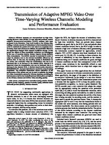
Figure 4 The parcel pipeline timing diagram for the plasma PIC application feeding a single SPELL. The parcel phases are taken in order from Table 6. The SPELL is kept busy by a sufficiently infinite stream of parcels supplied by the DPIM and SPIM layers.

We determined the subscription rates of the various resources in the architecture. First, for each of the five phases in the parcel pipeline we note the additional parallelism available. For example, the 281 µsec required for parcel assembly in the DPIM used a single processor out of the 128 available. These available parallelism factors are included in Table 6. To compute resource utilization, we normalized the time by the available parallelism factor. Normalized assembly time becomes 2.20 µ sec; normalized dispatch time becomes 0.59 µ sec. The largest of these overlapable parcel phase times is the normalized SPELL execution time, 14.2 µsec, meaning that the DPIM and SPIM are able to build and feed

24 parcels fast enough to keep the SPELLs busy. The resource utilization is simply the ratio of the normalized time and this largest normalized time, shown in the table. We emphasize that this normalization does not imply that we will actually spread the work for a single parcel across the available parallel resources at a given architectural layer. It assumes only that enough parcels will be in the pipeline to keep these resources sufficiently busy. Table 7 Summary of the plasma PIC problem size estimate. For a problem that must be held in DRAM without paging to and from HRAM, the problem size is limited as shown. To cycle once through all parcels in this dataset will take approximately 72 msec. A typical simulation might run for 10,000 time steps.

Slice (single SPELL) Parcel rate Particle rate DRAM limited: Particle Push Parcels Particles Field points Iteration time

Full HTMT

70 K/sec

288 M/sec

1.4 G/sec

5.9 T/sec

5K 80 M 5M

20 M 330 G 20 G

72 msec

Finally, scaling the one-slice analysis up to the full architecture, we can estimate the problem size accessible to this architecture. A single SPELL can compute approximately 70,000 parcels per second. The entire machine, configured with 4096 slices, can therefore compute 288 M parcels per second. We estimate that the total DRAM in a slice can manage of order 5,000 parcels for this problem. Each parcel represents 16,000 particles and 1,000 grid points. Summarizing salient results from Plasma PIC analysis: • • •

SPELLs will be 100% busy. For this code, with 88% of the inner loop devoted to floating-point operations, this means that we will sustain 88% of peak FLOP rate. A simulation of 330 billion particles on a grid of 20 billion field values could be be run using available DRAM. A 10,000-step run would take approximately 720 seconds. The assumptions in the analysis presented in this report result in a sustained performance of approximately 0.9 PFLOP per second for this application. The authors of the original application report came to the more conservative final performance estimate of 0.3 PFLOP per second. This discrepancy owes to our use of increased final DPIM and SPIM node counts per slice.

25

3.2.4 Volume Rendering The term volume rendering refers to a class of visualization techniques that present 3-D datasets in ways that illuminate the internal structure of the data (see, for example, Lichtenbelt, Crane, and Naqui 1998). These often involve some form of transparency. In the algorithm described here, the data consist of values on a regular 3-D grid of points. These may represent material density given by an MRI of a human head, the temperature of the fluid in a simulation of the interior of a star, the pressure of the atmosphere in a simulation of global weather, or any such scalar field in any number of measurement or simulation domains. Volume rendering in general need not be limited to scalar fields, but for this algorithm we consider only these sorts of data set. # -------------------------------------------------------------------------------------------------------------------------# volume rendering pseudocode # -------------------------------------------------------------------------------------------------------------------------foreach $pixel in ($plane) $frustum = f ($pixel, $plane, $viewpoint) $value = 0 $opacity = 1 foreach $voxel along ($frustum) $local = interpolate($data, $voxel) $value = $value + $local/$opacity $opacity = darken($opacity) if ( $opacity > $threshold ) exit end image_plane($pixel) = $value end

% 2-D pixel loop % compute pixel frustum from viewpoint % initialize pixel value to zero % initialize opacity % march outward along frustum % interpolate value of data at center of voxel % add to accumulating pixel value % increase opacity factor % compare opacity factor to threshold and exit % end voxel loop % save accumulated value in current pixel % end pixel loop

Figure 5 Summary of the serial rendering algorithm in pseudocode.

3.2.4.1 Serial Algorithm for Volume Rendering The approach taken in the serial volume-rendering algorithm is to cast rays through the data volume, one for each pixel to be rendered. With each ray is associated a frustum of included volume to be projected in some way onto the corresponding pixel in the image plane. In the case of orthonormal projection, these frusta become square tubes. Intensity is accumulated as the ray is traversed outward from the viewpoint and through the data, enabling a number of effects in which contributions from data within the volume are manifested visually in the final 2-D rendering. The algorithm accounts for arbitrary viewpoint. It is parameterized by an opacity factor that weights contributions in the foreground more heavily than those in the distance. A threshold test is included to allow early termination of the ray traversal if a test of the opacity determines that the data beyond will make no perceivable contribution or if the accumulated intensity is already at the maximum. Here is a quick summary of the algorithm as it might be implemented on a serial architecture (pseudocode in Figure 5). The outer loop of the algorithm iterates over the 2D array of pixel positions in the image being rendered. For each of these pixels a frustum is cast from the viewpoint through the image plane. The data in the frustum can

26 contribute to the computed pixel value. The inner loop walks outward from the image plane along the frustum centerline. At each step of this loop the data is interpolated and scaled to the voxel volume to compute the local contribution to the pixel value. This local contribution is adjusted by the present value of opacity before being accumulated into the computed pixel value. If the sum reaches the allowed maximum, then the inner loop is terminated. The opacity factor is increased at each step. If the opacity rises above a threshold parameter the inner loop is terminated early.

Image Plane

Of interest in the algorithm as presented here are bilinear interpolation, inclusion of the cutoff threshold, orientation of the regular data grid, the scale change as a result expanding volume of the frustum, and ray fragment management.

Viewpoint

Of particular interest is the fact that in this application the execution time (or Data Grid time to render a frame) depends on the data, the viewpoint, and the rendering Figure 6 Schematic showing rays cast parameters (such as opacity). through data. Consequently an estimate of the performance (for example, in terms of resource utilization) depends strongly on these conditions of the computation. 3.2.4.2 Performance Analysis of Volume Rendering on HTMT In a classical MPP algorithm one might assign a thread to each ray, particularly if the algorithm were implemented on a shared-memory machine. This approach is not possible on the HTMT, if only because of the space limitations within the CRAM. In this algorithm, the main parcel for the computation will be composed of a ray list and a 3-D subcube of the data. The DPIM will manage the data partitioning. The SPIM will manage ray accounting, orchestrate ordered gather of data from DPIM, dispatch parcels to SPELL, and scatter image plane results. Here is an outline of that process: 1. Viewpoint Broadcast. Information is broadcast to DPIMs, including the image plane information necessary to generate ray data. 2. Assemble. Each DPIM calculates for the voxels that it owns: the subcubes it needs to contribute, front-to-back ordering information based on viewpoint, and the rays passing through the subcube. 3. Gather. Each SPIM gathers from the DPIMs the subcubes oriented in line with the viewpoint. 4. Dispatch & Inject. SPIM dispatches to the SPELLs the subcubes in front-to-back order.

27

5. SPELL Execution. SPELL calculates the ray casting through the subcube: lighting, voxel properties, interpolation, and accumulate. 6. Eject. SPELL returns intermediate calculation of ray value accumulation and termination information. 7. Retire. SPIM holds the ray accumulation buffer for next subcube and adjusts ray tables to steer subcube dispatches. When all rays in the bundle have terminated, front-to-back subcube dispatch along this bundle terminates. 8. Scatter. SPIM composites and outputs the image to the Data Vortex. Because image patch is not ready until parcel processing along a ray bundle has terminated, this operation does not happen for every parcel. Our estimate of the time it takes to execute the principal volume rendering parcel reduces to the following model: TEXEC = α * NCYCLES * NG3 * tSPELL. From a bilinear interpolation kernel we find that NCYCLES is at least 22 – this is a lower bound on the number of cycles required to compute the contribution of a voxel to the accumulating ray value. We are using a value of 44. The factor α accounts for three effects: the number of rays being traversed, the effects of ray termination within the subcube, and scale changes in expanding arrays. It is a function of the data being visualized, rendering viewpoint, and opacity; we estimate it to be typically in the range 0.1 to 0.5. Using the following estimation of the time needed to move the parcel into the CRAM, one can find the portion of parameter space (if any) for which it is cost effective to execute the parcel: TMOVE = (WM + 6 *NR + 0.5 * NG3) * tS to C. The first term is the number of words of executable code in the parcel, the second is the space taken by ray data, and the third is the space taken by the subcube itself. It does not take a very large value of NG for the third term to dominate: probably between 10 and 100.

28 Table 8 Summary of parcel processing times for the volume rendering application.

Parcel Phase

Principal Resource

Assemble Gather Dispatch Inject SPELL Execution Eject Retire Scatter

DPIM DV (D Æ S) SPIM RTI (S Æ C) SPELL RTI (C Æ S) SPIM DV (S Æ D)

Work / Volume 99,500 80,500 25,000 80,500 2,200,000 15,000 25,000 75

Time cycles W cycles W cycles W cycles W

191 µsec 8 µsec 25 µsec 1.3 µsec 8.8 µsec 0.2 µsec 25 µsec 0.008 µsec

Avail. Parallel

Utilization

128 1 64 1 1 1 64 1

17 % 94 % 4.5 % 15 % 100 % 2.7 % 4.5 % 0.1 %

One concern is whether the cost to move a parcel into the SPELL is less than the time it takes for the SPELL to execute that parcel. In other words, is there sufficient reuse? We hope that TMOVE < TEXEC. For parcel size dominated by subcube data, this condition reduces to the following: α * NCYCLES > 0.5 * tS to C / tSPELL. For the parameters of our HTMT model, the right-hand side is approximately 2. With NCYCLES > 22, and α > 0.1, we conclude that we can expect the volume rendering parcels will use the computing resource of the SPELL effectively. On the other hand, the same parcel must be passed from the DPIM to the SPIM through the data vortex. For the analogous relation (replacing tS to C with tD to S) the right-hand side becomes approximately 13, which places the burden on the DPIM to supply parcels fast enough to keep the SPELL busy. For nominal values of the model parameters, the principal parcel of this application can be summarized by the time spent at the various layers in the architecture (Table 8). We can estimate the approximate size of the largest rendering job that the HTMT could support. At 8.8 msec per parcel, the 4096 SPELLs can process almost 500 million parcels per second. And at 24 frames per second, this corresponds to about 2.4 teravoxels per frame, or 180 megapixels per frame. If the rendered pixels fed an 8 foot by 7 foot display with 150 dpi resolution, we could interactively navigate through a volume-rendered dataset that was approximately 1.2 terawords (3 bytes per grid point).

3.3 Summary Evaluation of Application Performance Table 9 summarizes the equilibrium resource utilization for our four applications. As hoped for, the applications chosen exhibit a range of demands on the available resources. The Cannon algorithm and the SAR application involve many parcels. The values tabulated in Table 9 represent a suitable average of the individual parcels. In the case of

29 the SAR application, for example, we computed the aggregate utilization by weighting the individual parcel resource values with the time spent as a fraction of the total SPELL time. Note that the resource usage for the Read Patch and Write Patch parcels is almost entirely nonoverlapping with other parcel resource usage, and so these can be executed in parallel with the parcels that use SPELL time. For each Read Patch parcel executed, we are using 4096 Range Line and 11812 Azimuth Line parcel, the typical patch size. To summarize our impressions based on the applications analyzed, we revisit the questions posed in introducing the evaluation framework: Will the application perform well? All of the applications summarized here come close to extracting petaops performance out of the SPELL layer of the architecture. In this sense, the applications perform well, within the limitations of the present analysis. The volumerendering application stands out here as an example of an application on the edge. Its performance depends not only on the details of the data being visualizes but also on the particular viewpoint and visualization parameters selected by the user. As an interactive application (assuming the appropriate interfaces to a display device), the performance of the application can change. Table 9 Equilibrium HTMT resource utilization for applications in our suite. Application Summary Execution Time Processor Utilization Comm. Utilization

Memory Utilization

Matrix Multiply 750 µsec

Plasma PIC 55 msec

Volume Rendering 8.6 µsec 24 fps forever

100% 6% 22%

100% 9% 17%

16 sec

SAR 60 msec 15 µsec 82 sec

83 %

100%

17 %

6%

S => C S S D => S D D H => D H