Medical Image Analysis 4 (2000) 303–316 www.elsevier.com / locate / media
Phantom-based performance evaluation: Application to brain segmentation from magnetic resonance images Bruno Moretti
a,b ,
*, Jalal Mohamed Fadili a,b , Su Ruan a , Daniel Bloyet a , Bernard Mazoyer b,c a
´ Juin, F 14050 Caen Cedex, France GREYC-ISMRA UPRESA 6072, 6 Bd du Marechal b ´ , Caen, France GIN UPRES EA 2127, LRC 13 V-CEA /DSV, GIP Cyceron c ˆ de Nacre, Caen, France Unite´ IRM, CHU Cote
Received 26 May 1999; received in revised form 2 November 1999; accepted 18 February 2000
Abstract This paper presents a new technique for assessing the accuracy of segmentation algorithms, applied to the performance evaluation of brain editing and brain tissue segmentation algorithms for magnetic resonance images. We propose performance evaluation criteria derived from the use of the realistic digital brain phantom Brainweb. This ‘ground truth’ allows us to build distance-based discrepancy features between the edited brain or the segmented brain tissues (such as cerebro-spinal fluid, grey matter and white matter) and the phantom model, taken as a reference. Furthermore, segmentation errors can be spatially determined, and ranged in terms of their distance to the reference. The brain editing method used is the combination of two segmentation techniques. The first is based on binary mathematical morphology and a region growing approach. It represents the initialization step, the results of which are then refined with the second method, using an active contour model. The brain tissue segmentation used is based on a Markov random field model. Segmentation results are shown on the phantom for each method, and on real magnetic resonance images for the editing step; performance is evaluated by the new distance-based technique and corroborates the effective refinement of the segmentation using active contours. The criteria described here can supersede biased visual inspection in order to compare, evaluate and validate any segmentation algorithm. Moreover, provided a ‘ground truth’ is given, we are able to determine quantitatively to what extent a segmentation algorithm is sensitive to internal parameters, noise, artefacts or distortions. 2000 Elsevier Science B.V. All rights reserved. Keywords: Magnetic resonance image; Brain segmentation; Validation; Performance quantification
1. Introduction Accuracy in image segmentation is a nettlesome problem, especially in medical image analysis, where precision in segmentation is a prerequisite for a reliable interpretation of results. Moreover, many current problems in the medical realm and diagnosis derive benefit from a precise brain segmentation. For instance, delineating the anatomical structures in the vicinity of the entorhinal cortex helps neuroanatomists in the diagnosis of Alzheimer’s disease (Frisoni et al., 1999; Juottonen et al., 1999). Intracranial volume measurements in serial magnetic resonance images also need flawless segmentation, particularly for studies *Corresponding author. E-mail address:
[email protected] (B. Moretti).
and therapy monitoring in ischemic disease, vascular dementia, multiple sclerosis (Broderick et al., 1996), or mesial temporal sclerosis (Kuzniecky et al., 1996). Furthermore, the cortical surface detection in magnetic resonance images is of great importance for the quantification of sulcal lengths (Vannier et al., 1991), for three-dimensional brain display in image-guided neurosurgery (Galloway et al., 1992, 1993; Grimson et al., 1996) and in EEG projection (Jack et al., 1990). Similarly, multimodality image registration requires a good brain segmentation: indeed, surface matching techniques need to have a precise definition of the segmented volumes (Pelizzari et al., 1989; Mangin et al., 1994; Malandain et al., 1995; Turkington et al., 1995; De Munck et al., 1998). As a matter of fact, any image analysis technique has to be validated in an efficient way so as to legitimize its use in clinical day-to-day
1361-8415 / 00 / $ – see front matter 2000 Elsevier Science B.V. All rights reserved. PII: S1361-8415( 00 )00021-9
304
B. Moretti et al. / Medical Image Analysis 4 (2000) 303 – 316
applications. As stated by Barrett (1996), a rigorous definition of image quality in terms of algorithm efficiency depends on the performance of some observer on some specific task; and mathematical models for these observers have to be designed in order to replace humans. The lack of well-considered validation techniques is due to the fact that assumptions underlying the task at hand are not clearly defined (Jain and Binford, 1991). Moreover, the high level of automation in segmentation inherently introduces a number of impediments for validation (Gerritsen et al., 1995). This paper is organized as follows. In the first part, we address the fundamental problem of assessing the accuracy of brain segmentation methods. After a brief review of existing methodologies, we substantiate the need of a reference to quantify the performance of segmentation. Thanks to the Mac Connell Brain Imaging Center (Collins et al., 1998), we use a realistic MRI brain phantom that takes into account the well-known partial volume effect due to spatial sampling: each voxel of the phantom volume is assigned a known proportion for each cerebral tissue. Based on this model, deemed as the reference, we propose new criteria that allow us to assess the performance of segmentation algorithms in a more or less local manner by utilizing distance knowledge between the segmented brain and the reference. In the second part of the paper, we present a cooperative brain editing algorithm in a way akin to the methodology combining region growing and contour approaches (Pavlidis and Liow, 1990; Kapur et al., 1996). More precisely, the goal is to refine region growing step results thanks to active contours. The two stages enshrined in our segmentation method stand for a typical application of our evaluation procedure. By the same token, we expose the brain tissue classification method, the performance of which has been tested with our criteria. Finally, we present the results of the segmentation methods, on which the evaluation criteria are applied, and demonstrate the ability of these new measures to faithfully characterize the accuracy of the segmentation algorithms. Both phantom and real data are used, for which appropriate features are calculated, that take into account the propensity for active contours to more or less accurately delineate the brain cortical surface. A joint optimization for active contour parameters is performed, which gives a range of satisfying values according to the criteria used. Furthermore, the influence of data noise and non-uniformity on the quality of segmentation is studied. Finally, the powerful use of the brain phantom as a reference conjugated with distancebased evaluation procedures is discussed, and perspectives towards validation of other image analysis techniques are given.
2. Assessment of segmentation accuracy Because of the morphological complexity of the brain, the methods for validating the quality of segmentation are
limited. Comparisons are often made between results from the automatic segmentation and those obtained manually, taken as the standard reference. But the inter- and intraexpert variability is often biased toward the so-called performance of segmentation, which therefore does not allow us to define a reference very accurately. Furthermore, the ability to have a reference phantom, either physical or digital, does not ensure that quantitative measurements are possible in order to evaluate correct correspondence between the automatically segmented volume and the reference. Indeed, relevant criteria must both faithfully and precisely convey the global subjective impression on the quality of the segmentation and quantify its accuracy. This compelling trade-off makes the validation of segmentation a difficult and often dodged issue.
2.1. Related work Several investigators have worked on the evaluation of the segmentation quality in medical image analysis. Assessing the accuracy of segmentation algorithms is an open problem and different methods are detailed in (Zhang, 1994; Cho et al., 1997). According to van Gennip and Talmon (1995), the assessment of algorithmic accuracy in segmenting objects needs to apply the method to three types of data: artificial software-generated images, where the ‘ground truth’ is thoroughly known; hardware phantoms because of their more realistic design; and, finally, real images. In (Hoover et al., 1996) a ground truth is created from manual delineations, with the risk of bias due to expert variability. In (Heath et al., 1997) a statistically based method is proposed for evaluating five edge detection algorithms from visual rating scores indicated by participants on a set of gray-scale images. By the same token, Chalana and Kim (1997) suggest statistical methods to verify whether the computer-generated boundaries agree with the manually outlined contours. Indeed, the problem in human visual evaluation is that specifying the ground truth for real images is very difficult because subjective, not to mention the tedious work it entails for the experts to manually delineate the alleged true contours. Actually, some studies based on the use of a phantom have already been performed. In (Mortelmans et al., 1993) the clinical acceptance of a model-based myocardial border delineation method on SPECT images is described both with software and man-made phantoms. In (Disler et al., 1994) manmade phantoms of varying shapes are used and filled with different contrast agents to assess the volumetric capabilities of CT and MR imaging. Similarly, in (Kalender, 1992) the validation approach of segmentation accuracy is based on the use of the man-made European Spine Phantom, on which specific anatomically designed distances are calculated. Tofts et al. (1997) use obliquely oriented cylinders for measuring the accuracy of lesion volume estimation schemes. In (Chakraborty et al., 1996) synthetic images are generated to quantify the accuracy of
B. Moretti et al. / Medical Image Analysis 4 (2000) 303 – 316
305
the boundaries given by their gradient-based deformable boundary finding algorithm. According to the well-known description of the validation scheme (Haralick, 1994), smoothing and noise have been added in order to better simulate real data. The performance of the segmentation method was assessed from calculation of minimal distances of sampled points on the reference boundaries to the final segmented ones. Let us emphasize here that our quantification scheme basically hinges on this distance information.
defined as follows: one voxel belongs to the tissue Mi if the proportion of this tissue in the voxel is greater than 50%. This one-to-one relationship allows us to define unambiguous membership of a voxel to the corresponding tissue. In other words, a voxel belongs to one and only one tissue. In spite of this property, and since more than two different tissues make up the phantom (N . 2), an underlying voxel class is created, gathering all the voxels which do not belong to any predefined tissue, that is to say the (x,y,z) due to the partial volume effect such as
2.2. Digital brain phantom
; i [ n1,Nm, PMi (x,y,z) < 50%.
In our particular application, we have discarded any physical phantom, because the latter only attests geometric reliability, and usually does not take into account the intensity-based information of magnetic resonance images. Moreover, the use of a physical phantom necessarily needs a registration step to match the ideal physical object with the segmented one, and hence to quantify the performance of the segmentation algorithm used. Because we wanted to avoid the resulting inaccuracy added by registration and to have a phantom as realistic as possible, we have used a computationally synthesized phantom, the geometry and intensity of which at best express the results obtained by real MRI brain imaging systems. This phantom is available on the site Brainweb,1 which affords two data sets: on the one hand, the proportion volumes of each cerebral tissue, constituting the anatomical model; and on the other hand, the resulting volume, which we reckon as our brain phantom. Some choices for parameters are proposed, such as the spatial resolution. By specifying the modality type (T1-weighted as far as we are concerned), and by means of the Bloch equations (Bloch et al., 1946), representing the link between the physical nuclear magnetic resonance phenomena and the observed signals, it is possible to obtain the volume resulting from the chosen model (Kwan et al., 1996). The great advantage of this phantom model lies in the knowledge of the proportion of any cerebral tissue at discrete location of the volume. These proportions have been devised from a classification procedure performed on the mean volume of 27 registered T1-weighted MR volumes of one single patient (Collins et al., 1998), which led to a very high signal-to-noise ratio. Henceforth, the following notation is used concerning the phantom model: M 5 hMi j 1 (D
(4b)
where Bi is the sphere with radius equal to i and D Bi (Cr ) is the dilation of Cr by the sphere Bi . S int i 11 is the surface constituted of the voxels inside the volume of reference Vr whose distance to the contour Cr is i 1 1 voxels and which
will be indexed by 2 (i 1 1). S ext i 11 is the surface constituted of the voxels outside the volume of reference Vr whose distance to the contour Cr is i 1 1 voxels and which will be indexed by i 1 1. In that way, iso-intensity surfaces (see Fig. 1(a)) are created, each voxel of which is coded by its distance to the reference contour Cr . The construction of the SDM ensures that the distance is that of the closest point to the contour (Fig. 1(b) and 1(c)). By superimposing this SDM to the contour Co , a grey-level intensity contour geometrically identical to the latter is obtained, but for which each voxel intensity represents its distance to the reference contour Cr . Hence it is quite easy to make this distance information visible by displaying the 3D resulting distance contour (DC), and to see local discrepancies of the object volume Vo in relation to the reference Vr (Fig. 1(d)).
2.3.2.2. Distance histogram. Because of the huge amount of local information resulting from the formerly presented SDM, the distance contour DC cannot directly provide an assessment of the accuracy of the segmentation algorithm. Furthermore, a visual inspection would not make a significant improvement to the usual comparison between the manually delineated contours and the results. Thus, one must extract from the raw data some relevant characteristics, which should be as discriminating as possible towards unbiased criteria. The most simple means to compress distance information is to calculate the distance histogram of DC, which indicates the number of voxels in Co at any distance of Cr . In other words, the distribution of distance errors of Co in comparison with Cr is obtained, and their similarity can then be assessed. 2.3.2.3. Model-based measurement method. We have only taken into account the distance concept in order to compare a test volume with a ‘ground truth’. Now, the issue of segmentation methods is that of extracting the brain from the cranium. The goal is to delineate the external cortical limit (grey matter), contained in the cerebrospinal fluid (CSF). This interface notion, combined with the phantom model, led us towards the use of the notion of percentage of matter per layer. The idea is to take into account, in addition to the distance information, the proportion of each matter given by the phantom model, in order to characterize the similarity between an edited volume and the ideal brain. In order to most profitably use the phantom model, iso-distance layers from the contour Cs of the segmented volume Vs were created in the same way as the iso-intensity surfaces used in the previous section. In this way, the delineation of encephalon, considered as the edge between grey matter and cerebro-spinal fluid (CSF), ext is obtained. For each layer inside (outside) S int i 11 (S i 11 ) the segmented volume Vs , the histograms of the grey matter and CSF proportions per 5% slices are created, that is the number of voxels in the considered layer that have a
B. Moretti et al. / Medical Image Analysis 4 (2000) 303 – 316
307
Fig. 1. (a) Building of the distance map of the reference at step i; (b) Signed Distance Map (SDM) on the reference contour (in black); (c) 3D Signed Distance Map (SDM) applied on the encephalon reference contour (in white). Colour coding of the distance holds from 220 to 120 voxel; (d) Distance Contour (DC) of an edited brain in relation to the reference.
proportion of grey matter (CSF) between 50 and 55%, 55 and 60%, etc. For each tissue, 10 classes Cj are obtained: Cj 5 ]b j ,b j 11 ], b j 5 50 1 5j, 0 < j < 9. The number of voxels in the layer Si belonging to the tissue M in class Cj is then n CSij (M) 5 [hV(x,y,z) [ Si , PM (x,y,z) [ Cj j.
(5)
The total number of voxels in the layer belonging to the tissue M verifies
On 9
n Si (M) 5
j 50
Cj Si
(M).
(6)
Therefore, for each layer, it is possible to define the number of voxels of each tissue as its proportion associ-
ated class. Furthermore, normalizing n CSij (M) by n Si (M) gives the percentage of voxels of any structure M belonging to the class Cj .
2.3.3. Overall statistical features Now, from the distance histogram detailed above, one must extract some relevant data that sum up its global behaviour, so as to obtain a discriminating vector for each distance histogram. These characteristics must attest as faithfully as possible the performance of the segmentation, even though they cannot ensure that the accuracy is absolute. At least, if one of the coordinates of the resulting discriminating vector is significantly bad with respect to our criteria, we are then able to conclude that the segmentation has failed in a precise manner, depending on the significance of the unsatisfactory characteristic.
308
B. Moretti et al. / Medical Image Analysis 4 (2000) 303 – 316
2.3.3.1. Mean error. The first statistical measure to be naturally extracted from the distance histogram is the mean of the error distribution. This first-order moment gives information on the global behaviour of the segmented contour. In other words, one can imagine an equivalent contour equidistant to the reference contour, with the same mean error as the segmented contour, but with other higher-order moments null (e.g., the variance): the mean error isocontour. If the absolute value of the mean error is higher than a given threshold, it means that the number of voxels far away from the reference is substantial, and that the segmentation is unreliable. Of course, a subjective threshold is necessary to reject a segmentation. This means that the operator will have to decide whether the chosen threshold is relevant or not. But it is clear that there is no ideal value: it depends on the wishes of the user. 2.3.3.2. Standard deviation of the error. The most usual second-order statistical moment is the standard deviation of the error distribution, which is representative of the spreading of the histogram. Its interpretation is quite simple: the greater the standard deviation, the sparser the voxels of the contour around the mean error isocontour and, hence, the worse the segmentation. So, in the case of a low mean error in the segmentation, a too high standard deviation means that there are many outliers on the segmented contour, and that the segmentation procedure has failed in a way proportional to the variance. Nevertheless, a low standard deviation must also be defined with a threshold, which is another parameter. 2.3.3.3. Skewness and kurtosis. Even though the two former statistical moments are usually enough to describe the behaviour of a distribution, we have calculated the third moment (or skewness) and the fourth moment (or kurtosis) of the distance histogram, so as to more precisely characterize the segmentation performance. The skewness, whose value determines the degree of asymmetry of a distribution around its mean, is useful to test whether the distance errors mostly stand inside or outside the reference contour. As for the kurtosis, it indicates the relative peakedness or flatness of the distribution, and hence is representative of the importance of the ‘small’ segmentation errors. The more the small errors, the lower the kurtosis. But a high positive kurtosis is not indicative of a good segmentation. 2.3.3.4. Distance to the maximum. That is why the distance to the maximum error is relevant: it can attest to the worst segmentation error and show in which manner the segmentation has failed. But, as the final segmented surface is closed and continuous, as far as the discrete topology is concerned, one voxel far away from the reference contour implies that its direct neighbours also stand far away from the ideal contour and, therefore, that many substantial segmentation errors inevitably occur.
Consequently, a high value for the maximal distance error can lead to a peaked histogram, but usually entails a high value for the standard deviation and low (negative) value for the kurtosis. As a conclusion, we have processed some characteristics from the distance histogram. No precept is to be followed a priori to find the ‘best’ segmentation. Actually, the conjunction of the proposed tools can be used advisedly to obtain the performance of the segmentation algorithms. They only allow the rejection of a segmentation for a particular criterion, but cannot ensure that the segmentation is satisfactory according to other criteria, as yet undefined.
3. Tested segmentation methods A huge number of studies have already been carried out concerning 3D MR segmentation, from most of which it emerges that the stumbling block in MRI data comes from the morphological complexity of the brain, which includes both smooth and jagged areas. Segmentation of the encephalon is usually performed in three ways. The first one is based on region growing techniques and connectivity rules (Cline et al., 1987; Joliot and Mazoyer, 1993). Nevertheless, a manual operation is often required in order to cut the undesirable ties caused by partial volume effects. The second method deals with contour detection using gradient or Laplacian (Bomans et al., 1990; Raman et al., 1991), but needs a post-processing. Finally, the last method, based on mathematical morphology (Brummer et ´ al., 1993; Verard et al., 1995), consists of two main steps: a threshold followed by erosions in order to disconnect the different cerebral structures, and conditional dilations to obtain a complete structure and retrieve illegitimately broken ties.
3.1. Editing algorithm The first step of our cooperative segmentation method consists in obtaining the initial contour for a further refinement with active contours. The methodological approach is based on a histogram analysis for an automatic threshold selection and on morphological steps (Suzuki ´ and Toriwaki, 1991; Verard et al., 1995; Aboutanos and Dawant, 1997). The former contour is then submitted to internal constraints linked to the regularization of the contour and to external constraints involving local properties in terms of image knowledge. The active contours model, originally introduced by Kass et al. (1988), has been applied in many fields, and particularly in segmentation (Cootes et al., 1994; Ashton et al., 1997). It is to be pointed out that authors often ignore the crucial choice of parameters of the deformable model, which is the backbone of segmentation. In the deformable model we have implemented (Nastar and Ayache, 1992), each point
B. Moretti et al. / Medical Image Analysis 4 (2000) 303 – 316
belonging to the contour is given a physical mass, linked to its neighbors by springs, and converging towards a stable state under an external strength field. Because of the time requirement heaviness of active surface, we only applied active contours in 2D in a slice-by-slice method along the axial axis. The evolution of each mass m i is described by the well-known equation Fi (t) 5 m i a i (t), 0 < i < n,
(7)
where Fi (t) is the total strength applied on the point Mi and a i (t) its acceleration. Assuming that all the points of the contour have unit mass and the same damping coefficient, the nodal shifting Ui (t) 5 Mi (t) 2 Mi (t 0 ) of each point Mi (t 0 is the initial instant) is ruled by the second-order differential equation F ext i (t) 5 U i99 (t) 1 2zvn U i9 (t) 2 n
1 v (2Ui 21 (t) 1 2Ui (t) 2 Ui 11 (t)),
(8)
(9)
where a (a [ [0,1]) balances the image and gradient knowledge. The minus sign in the gradient potential formula means that the contour must tend towards strong gradients with low grey values, that is to say towards CSF, which is a prerequisite for encephalon extraction. The invariability of a in formula (9) would imply undesirable constraints in the simple implementation of this method. Indeed, depending on the value a, either the image potential or the gradient potential is emphasized: a weak a (a < 1) will lead the active contours towards strong gradient areas, whereas a high value (a . 1) will drive it to low-intensity areas. Now, the compulsory trade-off it implies must not be indefinitely fixed, given a contour, but rather locally adjustable according to image characteristics. Therefore, we have made a dependent on the local gradient, more precisely as a decreasing function of the gradient: a equals 1 where the gradient information is insignificant and converges to 0 when the gradient norm tends towards infinity. The chosen function is then the following: 1 a! (grad(M)) 5 ]]]]]], 1 1 [igrad(M)i /! ]
locally modifies the weight of both image and gradient potential.
3.2. Brain tissue segmentation As we wanted to evaluate the performance of intrinsically volumetric structures segmentation, we implemented a classification algorithm that utilizes three-dimensional Markov Random Field (MRF) models for segmenting cerebro-spinal fluid, grey matter and white matter in magnetic resonance T1-weighted images. The mixclasses (mixture of two pure classes), due to the partial volume effect, are taken into account in the tissue class model. The method is thoroughly described in (Ruan et al., 1998).
4. Results
where z is the damping factor and vn the natural pulsation of the system. The excitation field arises from one or more image properties, and is derived from the potential Pt associated with the strength field Fext (t) 5 2=Pt , where = is the gradient operator. As far as we were concerned, this potential was chosen as a linear combination of an image potential and a gradient potential: Ptotal (M,t) 5 a I(M,t) 2 (1 2 a )i=G *s I(M,t)i,
309
(10)
where ! acts as a normalization factor that can be calculated from global attributes on the gradient image. Thus, we have built an adaptive balance parameter that
The characteristics of the phantom used are as follows: T1-weighted MRI data, 1 mm thickness, l31 mm 2 inplane resolution (that is to say a 18132173181 volume), 8 bits per voxel (256 grey levels). The phantom, whose characteristics have been described in Section 2.2, is first used without any additive noise. In a first step, the initialization editing program gives the start contour for the active contours segmentation algorithm. Then, active contours are performed in a 2D slice-by-slice procedure in order to retrieve the grey matter missed by the first segmentation procedure. Even though the volume edited by the latter is simply connected, the 2D procedure makes some surfaces not simply connected (that is to say containing one hole at least). The resulting multicontour images are automatically processed for each slice. Finally, the brain tissue classification procedure is performed. For practical reasons, the 3D distance map of the reference volume has been performed in a maximal vicinity of 20 voxels: only the voxels whose distance to the reference contour is less than 20 mm are indexed as described in Section 2.3.2. In this way, 20 internal layers and 20 external layers are defined for the reference contour. Fig. 1(c) displays the distance map obtained, from which one-eighth of the space has been removed, in order to appreciate the global look of a typical map. The distance contour of the edited brain can elicit astonishment if no caution is taken (Fig. 1(d)). Indeed, the interpretation of the DC is not as straightforward as it might seem. Actually, one must keep in mind that a distance contour displays the distance discrepancies between an edited volume and a reference. From this, we can make two statements: the more homogeneous the color of a DC, the more homogeneous the error distance on the DC; secondly, the lower the absolute value of a voxel intensity, the closer to the reference the voxel is. The stumbling block of segmentation methods, i.e. the choice of appropriate parameters, is presented and discussed below for the editing operation. Concerning the
310
B. Moretti et al. / Medical Image Analysis 4 (2000) 303 – 316
tissue classification, we show some performance measures, and test the influence of well-known artefacts on segmentation performance. To finish, an application to real MRI images extends our criteria to assess the performance of the day-to-day editing procedure.
4.1. Parameter choice and joint optimization The use of active contours is always a crucial issue because it first requires to find, if not optimal, then at least satisfactory parameters. In order to obtain an appropriate range for vn , z and !, we have made these parameters vary by covering a parameters cube (subset of R 3 ) and calculating some features from the resulting distance histograms. The extremal values and steps for each parameter are the following: vn varies from 0.25 to 5, with the step dvn 5 0.25; z varies from 0 to 1, with the step dz 5 0.05; ! varies from 0.25 to 1, with the step d! 5 0.05. As the calculating process would be too long for the entire volume, we restrict our parameter optimization to the two-dimensional case by choosing and segmenting a representative axial slice of the tested volume. We then obtain a vector of performance characteristics at any point of the parameter cube, which allows us to find an optimal parameter set: the intersection of all the characteristic volumes thresholded to adequate chosen values, depending on the requirements of the user. Finally, the set of points in the parameters cube, whose resulting performance values verify our criteria, can be considered as a set of all possible values for the parameters. Thanks to the similarity measurements previously detailed, we succeed in determining a parameter set providing satisfying results with regards to the segmentation performance on the selected slice. The results are presented in Fig. 2, where the color map is defined by the usual correspondence: the darker the image, the lower the value. The five quantities on the distance histogram (mean, standard deviation, skewness, kurtosis, and maximum distance) are visible according to the three parameters of the active contours algorithm. As no volume can be visualized, we have decided to show only three slices in orthogonal directions, centred in the middle of the parameter cube. So, in each incidence (corresponding to one parameter), the influence of the two other parameters on the performance measures is shown. These images need some interpretation. To begin with, it is clear that the five characteristics are correlated. For instance, the maximum distance behaves in a way akin to the standard deviation, a phenomenon we have already expressed in Section 2.3.3. According to the mean variations, one can predict that low values for ! give better results (low mean). By the same token, one can expect values for the two other parameters (vn and z ) that are not too small. Otherwise, the mean error becomes too big, and the corresponding criterion is no longer verified.
Concerning the standard deviation, the same propensity is found for the good range of parameters. As regards the higher-order statistical measures, the skewness images show that the lower absolute values, corresponding to symmetric distance histograms, coarsely correspond to the low means and standard deviations. In the same way, the kurtosis images corroborate the remark in Section 2.3.3, and the high standard deviations (linked to the maximum distances) are equivalent to low negative kurtosis, which means that the distance histogram is platykurtic (flat distribution). Finally, there exists a good correspondence between each characteristic used. For purposes of visualization, we have tried to use two sets of parameters (Fig. 3), in order to illustrate the previous behaviour of parameters: one bad editing (with a satisfying standard deviation of 0.95, but a bad mean of 4.1), and one satisfying these statistical criteria (standard deviation 1.05, mean 1.15). The results of the brain editing are shown on the original slices, which are corroborated by the performance measures: the contour given by the bad editing obviously stands far away from the ideal contour. Let us specify here that the corresponding parameters were chosen according to the characteristics volumes previously described (Fig. 2), and the predicted effect of such parameters were verified on the original slices. Thus, the thought process used here is the inverse of the usual empirical one: we do not find the ideal parameters a posteriori, after any visual test, but a priori, from the joint optimization.
4.2. Three-dimensional extension We then make the assumption that the results obtained for the parameter optimization on an axial slice are extendable to the entire volume. One sufficient condition is that all of the possible geometrical and intensity-based configurations of the brain contour should be present in the tested slice, in such a way that no significant difference appears in the other slices of the whole volume. We present the distance histograms of the three-dimensional edited brain for each parameter set in Fig. 3(d). Some apposite remarks are now imperative. As foreseeable, the characteristics of the distance histogram have changed in relation to the two-dimensional restriction (Fig. 3(c) and 3(d)), especially by the fact that the means have significantly decreased, even though their trend to attest faithfully the segmentation performance is obvious. One hypothesis for this is that the two-dimensional joint optimization uses a two-dimensional distance map, whereas the three-dimensional performance histograms are calculated in a threedimensional way. So, some of the points belonging to the 2D test contour might be closer to the 3D cortical surface than when they were restricted to the two-dimensional case, especially for the points near a surface element almost tangent to the axial slice.
B. Moretti et al. / Medical Image Analysis 4 (2000) 303 – 316
311
Fig. 2. Joint optimization and orthogonal slices of variations of the statistical features according to the three parameters of active contours. The extremal values of the parameters set are: 0.25 < vn < 5, 0 < z < 1, 0.25 < ! < 1.
4.3. Brain tissue classification Once the brain editing has been performed, and with the concern to take into account the real acquisition phenomena, necessary for a reliable modelling, we apply the classification algorithm explained in Section 3.2, and test
its robustness in relation to the noise and the non-uniformity level. We utilize the data available on Brainweb, the noise varying with the following values: 1, 3, 5, 7 and 9%. Concerning the intensity non-uniformity, only two values are tested: 0 and 20%. For all of these configurations, we calculate the distance histograms for each usual
312
B. Moretti et al. / Medical Image Analysis 4 (2000) 303 – 316
Fig. 3. Influence of the parameters of active contours on the performance criteria for the active contours algorithm. (a) Bad editing result with vn 5 4.5, z 5 0.85, ! 5 0.9. (b) Good editing result with vn 5 5, z 5 0.6, ! 5 0.05. (c) Corresponding distance histograms with the following characteristics: (bad editing) mean 4.1, standard deviation 0.95, maximum distance 7, skewness 20.5, kurtosis 2; (good editing) mean 1.15, standard deviation 1.05, maximum distance 6, skewness 0.9, kurtosis 2.4. (d) Three-dimensional distance histograms of the previous ‘bad’ and ‘good’ editing, with the following characteristics: (bad editing) mean 2.247, standard deviation 1.489, maximum distance 7, skewness 20.5181, kurtosis 0.13; (good editing) mean 20.0649, standard deviation 0.9404, maximum distance 7, skewness 0.699, kurtosis 1.324.
cerebral matter (cerebrospinal fluid, grey matter, and white matter). The distance maps for all these internal structures are calculated from the definition of a reference contour, as specified in Section 2.3.2, by a threshold to 50% of each proportion volume. The influence of the two artefacts on the distance histograms is presented through its statistical features in Fig. 4. The first remark we can make from these variations is that the mean error almost equals 21, which means a bias of 1 mm in the detection of the contours. This phenomenon can be explained by the definition of the reference contour: the border of each cerebral matter is found by thresholding the original proportion volume to 50%. By the way, this threshold might have been too high, for each structure, and hence biases the performance quantification by an offset of one voxel. If only one classified matter had a positive offset, and the neighbouring structure the opposite of this offset, one could have concluded a bad classification. But, in our case, the same offset appears in each distance
histogram, which prompts us to adopt the aforementioned explanation. Next, for an intensity non-uniformity equal to 20%, one notes the global increase of the standard deviation while the noise increases. One possible explanation is that the number of well-classified voxels decreases (maximum of the peak), whereas the tails of the histograms grow substantially, and hence the variance increases. Moreover, this phenomenon is all the more pronounced for the cerebro-spinal fluid and the white matter. Anyway, it means that the non-uniformity artefact noticeably influences the performance of the classification process. We can conclude that the noise addition tends to shift some wellclassified voxels from the peak towards the tails of the distance histogram, and that this propensity increases with the intensity non-uniformity. Nonetheless, in view of the noise level tested on the magnetic resonance images, the classification results are quite satisfying, and we believe that our segmentation method is robust in relation to
B. Moretti et al. / Medical Image Analysis 4 (2000) 303 – 316
313
Fig. 4. Influence of the noise (N) and intensity non-uniformity (INU) on the statistical quantities of the distance histograms for the brain tissue segmentation, N varying in the range 1, 3, 5, 7 and 9%; INU is equal to 0 or 20%. (a) Mean variations for the cerebro-spinal fluid. (b) Standard deviation for the cerebro-spinal fluid. (c) Mean variation for the grey matter. (d) Standard deviation for the grey matter. (e) Mean variations for the white matter. (f) Standard deviation for the white matter.
314
B. Moretti et al. / Medical Image Analysis 4 (2000) 303 – 316
normally distributed white noise, provided on Brainweb. Nevertheless, an exhaustive study concerning the real noise effect should be performed. For instance, Rayleigh distribution for the background noise (Henkelman, 1985) should be added to the noiseless data.
4.4. Application to real MRI images For real experiments, the MRI images were acquired on a 1.5 T Signa scanner (GE-Milwaukee) using a conventional head-coil. We have used 25632563124 sized volumes, coded on 8 bits, with a 13131.2 mm 3 resolution, coming from 3D SPGR T1-weighted acquisitions (TE57 ms, TR530 ms, a 5 408). The aim of our study consists in showing the improvement in brain editing thanks to the active contours. Figs. 5(a) and 5(b) show results on a segmented volume axial slice, before and after the active contours step. The original program erodes the encephalon in the cortical area too much, that is to say
some gyri are not totally included in the final edited brain. On the contrary, the refinement using the active contours allows us to retrieve some omitted cortical parts. Furthermore, the geometrical complexity of the external cortical frontier (grey matter–cerebro-spinal fluid interface) is better managed by the active contours. By the way, it should be noted that the latter tends to include, in some places of the encephalon, some CSF, proclivity which can be explained by the form of the gradient potential in Eq. (9). Keeping in mind that the final purpose is to obtain the whole of the cerebral structures (especially the cortex) for a better subsequent classification of tissues, the advantage of active contours is obvious. Even though real data inherently cannot provide an unbiased ‘ground truth’, we have manually built a reference volume thanks to the Voxtool software.2 This refer-
2
Voxtool Software, General Electric, Milwaukee, WI, USA.
Fig. 5. Comparison of the two segmentation stages on real MRI T1-weighted data. (a) Superimposition of the contour before the active contours on the original axial slice. (b) Superimposition of the contour after the active contours on the original axial slice. (c) 3D distance histogram of the two former segmented volumes.
B. Moretti et al. / Medical Image Analysis 4 (2000) 303 – 316
ence has been devised by an expert, and helps us to use the distance-based criteria developed in Section 2. So, we have to make the assumption that this volume stands for a reference, whose accuracy is better than the mean error to be detected in the automatically edited brain. Now, considering the distance histograms (see Fig. 5(c)), it is obvious that many voxels before the active contours procedure extend too much into the reference volume. Conversely, the distance histogram of the edited brain after active contours shows that most voxels of the resulting surface belong to the reference contour, and most of the misclassified voxels have been retrieved.
315
paring one segmentation with a reference) or general registration (by testing the good fit between the standard and the resliced objects).
Acknowledgements We are grateful to the MR unit at Caen Hospital for providing the brain images used in this work. We also thank the devisers of the brain phantom available on the Web.
References 5. Conclusion and discussion To conclude, the contribution of this work to the evaluation of segmentation performance is shown, and the criteria used here can be a good prerequisite for validation of new algorithms, provided a reference is given. For purposes of validation, the use of a phantom model based on anatomical information of the brain and its synthesis from the physical equations provide a simulation as close as possible to the real acquired images. Moreover, the knowledge of all proportions of the cerebral matters in any location of the phantom permits us to precisely characterize the performance of the encephalon segmentation methods. Indeed, new methods for quantifying segmentation algorithms, combining the concept of distance and the information provided by the model, are presented. Furthermore, we use some statistical measures from the distance histograms to reliably find a set of optimal parameters according to user-defined criteria. Some examples show the faithful congruence between the performance measures and the effective accuracy of the segmentation. The robustness of a brain tissue segmentation algorithm with regard to some usual artefacts is tested and demonstrated with our performance evaluation method. Finally, we prove the efficiency of the brain editing method on real MRI images, by automatically comparing the results before and after the active contours step with a quasimanually designed reference. The distance information, provided by the definition of a reference, considerably improves the quantification of the segmentation performance. By means of some statistical features on the distance histograms, we can evaluate in which manner the segmented objects fit the ideal ones. The localization of the misclassified voxels can lead to an automatic enhancement of the segmentation process. The preselection of a range for parameters of active contours by means of the phantom is specific to the type of sequence. The extension of the phantom model presented here to other clinical day-to-day sequence types could provide a wider automation of the active contour method. More generally, the discrepancy measurements allow us to compare any kinds of objects, such as segmentation performance quantification (by com-
Aboutanos, G.B., Dawant, B.M., 1997. Automatic brain segmentation and validation: image-based versus atlas-based deformable models. IEEE Proc. SPIE-Med. Imaging 3034, 299–310. Ashton, E.A., Parker, K.J., Berg, M.J., Chen, C.W., 1997. A novel volumetric feature extraction technique with applications to MR images. IEEE Trans. Med. Imaging 16 (4), 365–371. Barrett, H.H., 1996. Objective evaluation of image quality. In: Second IEEE EMBS International Summer School on Biomedical Imaging. Berder Island, France. Bedekar, A.S., Haralick, R.M., Ramesh, V., Zhang, X., 1994. A bayesian corner detector: theory and performance evaluation. ARPA 94, 703– 715. Bloch, F., Hansen, W.W., Packard, M., 1946. The nuclear induction experiment. Phys. Rev. 70, 474–485. Bomans, M., Hohne, K.H., Tiede, U., Riemer, M., 1990. 3-D segmentation of MR images of the head for 3D display. IEEE Trans. Med. Imaging 9, 177–183. Borgefors, G., 1986. Distance transformations in digital images. Comput. Vision Graph. Image Process. 34, 344–371. Broderick, J.F., Narayan, S., Gaskill, M., Dhawan, A.P., Khoury, J., 1996. Volumetric measurement of multifocal brain lesions. Implications for treatment trials of vascular dementia and multiple sclerosis. J. Neuroimaging 6 (1), 36–43. Brummer, M.E., Mersereau, R.M., Eisner, R.L., Lewine, R.R.J., 1993. Automatic detection of brain contour in MRI data sets. IEEE Trans. Med. Imaging 12 (2), 153–166. Chakraborty, A., Staib, L.H., Duncan, J.S., 1996. Deformable boundary finding in medical images by integrating gradient and region information. IEEE Trans. Med. Imaging 15 (6), 859–870. Chalana, V., Kim, Y., 1997. A methodology for evaluation of boundary detection algorithms on medical images. IEEE Trans. Med. Imaging 16 (5), 642–652. Cho, K.J., Meer, P., Cabrera, J., 1997. Performance assessment through bootstrap. IEEE Trans. Pattern Anal. Mach. Intell. 19 (11), 1185– 1197. Cline, H.E., Dumoulin, C.L., Hart, Jr. H.R., Lorensen, W., Ludke, S., 1987. 3D reconstruction of the brain from magnetic resonance images using a connectivity algorithm. Magn. Reson. Imaging Magnet 5 (5), 345–352. Collins, D.L., Zijdenbos, A.P., Kollokian, V., Sled, J.G., Kabani, N.J., Holmes, C.J., Evans, A.C., 1998. Design and construction of a realistic digital brain phantom. IEEE Trans. Med. Imaging 17 (3), 463–468. Cootes, T.F., Hill, A., Taylor, C.J., Haslam, J., 1994. The use of active shape models for locating structures in medical images. Image Vision Comput. 12 (6), 355–366. De Munck, J.C., Verster, F.C., Dubois, E.A., Habraken, J.B., Boltjes, B., Claus, J.J., Van Herk, M., 1998. Registration of MR and SPECT without using external fiducial markers. Phys. Med. Biol. 43 (5), 1255–1269.
316
B. Moretti et al. / Medical Image Analysis 4 (2000) 303 – 316
Disler, D.G., Marr, D.S., Rosenthal, D.I., 1994. Accuracy of volume measurements of computed tomography and magnetic resonance imaging phantoms by three-dimensional reconstruction and preliminary clinical application. Invest. Radiol. 29 (8), 739–745. Eggers, H., 1998. Two fast Euclidean distance transformations in Z2 based on sufficient propagation. Comput. Vision Image Understanding 69 (1), 106–116. Frisoni, G.B., Laakso, M.P., Beltramello, A., Geroldi, C., Bianchetti, A., Soininen, H., Trabucehi, M., 1999. Hippocampal and entorhinal cortex atrophy in frontotemporal dementia and Alzheimer’s disease. Neurology 52 (1), 91–100. Galloway Jr., R.L., Maciunas, R.J., Edwards II, C.A., 1992. Interactive image-guided neurosurgery. IEEE Trans. Biomed. Eng. 39 (12), 1226– 1231. Galloway Jr., R.L., Edwards II, C.A., Lewis, J.T., Maciunas, R.J., 1993. Image display and surgical visualization in interactive image-guided neurosurgery. Opt. Eng. 32, 1955–1962. Ge, Y., Fitzpatrick, J.M., 1996. On the generation of skeletons from discrete Euclidean distance maps. IEEE Trans. Pattern Anal. Mach. Intell. 18 (11), 1055–1066. Gerritsen, F.A., van Veelen, C.W.M., Mali, W.P., Bart, A.I.M., de Bliek, H.L.T., Buurman, J., van Eeuwijk, A.H.W., Hartkamp, M.J., Lobregt, S., Moreira Pereira Ramos, L., Polman, L.J., van Rijen, P.C., Visser, C.P., 1995. Some requirements for and experience with COVIRA algorithms for registration and segmentation. In: Beolchi, L., Kuhn, M.H. (Eds.), Medical Imaging, pp. 4–27. Grimson, W.E.L., Ettinger, G.J., White, S.J., Lozano-Perez, T., Wells, W.M., Kikinis, R., 1996. An automatic registration method for frameless stereotaxy, image guided surgery, and enhanced reality visualization. IEEE Trans. Med. Imaging 15, 129–140. Haralick, R.M., 1994. Dialogue: performance characterization in computer vision. Comput. Vision Graph. Image Process.: Image Understanding 60 (2), 245–265. Heath, M.D., 1996. A robust visual method for assessing the relative performance of edge detection algorithms. Master’s Thesis, Tampa, FL. Heath, M.D., Sarkar, S., Sanocki, T., Bowyer, K.W., 1997. A robust visual method for assessing the relative performance of edge-detection algorithms. IEEE Trans. Pattern Anal. Mach. Intell. 19 (12), 1338– 1359. Henkelman, M., 1985. Measurement of signal intensities in the presence of noise in MR images. Med. Phys. 12 (2), 232–233. Hoover, A., Gillian, J.-B., Jiang, X., Flynn, P.J., Bunke, H., Goldgof, D.B., Bowyer, K., Eggert, D.W., Fitzgibbon, A., Fisher, R.B., 1996. An experimental comparison of range image segmentation algorithms. IEEE Trans. Pattern Anal. Mach. Intell. 18 (7), 673–689. Huttenlocher, D.P., Klanderman, G.A., Rucklidge, W.J., 1993. Comparing images using the Hausdorff distance. IEEE Trans. Pattern Anal. Mach. Intell. 15 (9), 850–863. Jack, C.R., Marsh, W.R., Hirschom, K.A., Sharbrough, F.W., Cascino, G.D., Karwoski, R.A., Robb, R.A., 1990. EEC scalp electrode projection onto three-dimensional surface rendered images of the brain. Radiology 176 (2), 413–418. Jain, R.C., Binford, T.O., 1991. Ignorance, myopia and naivete in computer vision systems. Comp. Vision Graph. Image Process.: Image Understanding 53 (1), 112–117. Joliot, M., Mazoyer, B., 1993. Three-dimensional segmentation and interpolation of magnetic resonance brain images. IEEE Trans. Med. Imaging 12 (2), 269–277. Juottonen, K., Laakso, M.P., Partanen, K., Soininen, H., 1999. Comparative MR analysis of the entorhinal cortex and hippocampus in diagnosing Alzheimer disease. Am. J. Neuroradiol. 20 (1), 139–144. Kalender, W., 1992. A phantom for standardization and quality control in peripheral bone measurements by QCT and DXA: Design considerations and specifications. Med. Phys. 19, 583–586.
Kanungo, T., Jaisimha, M.Y., Palmer, J., Haralick, R.M., 1995. A methodology for quantitative performance evaluation of detection algorithms. IEEE Trans. Image Process. 4 (12), 1667–1674. Kapur, T., Grimson, W.E.L., Wells III, W.M., Kikinis, R., 1996. Segmentation of brain tissue from magnetic resonance images. Med. Image Anal. 1 (2), 109–127. Kass, M., Witkin, A., Terzopoulos, D., 1988. Snakes: active contour models. Int. J. Comput. Vision, 321–331. Kuzniecky, R.I., Burgard, S., Bilir, E., Morawetz, R., Gilliam, F., Faught, E., Black, L., Palmer, C., 1996. Qualitative MRI segmentation in mesial temporal sclerosis: clinical correlations. Epilepsia 37 (5), 433– 439. Kwan, R.K.S., Evans, A.C., Pike, G.B., 1996. An extensible MRI simulator for post-processing evaluation. In: Visualization in Biomedical Computing. Fourth International Conference Proceedings. Lecture Notes in Computer Science, Vol. 1131. Springer, pp. 135–140. Malandain, G., Fernandez-Vidal, S., Rocchisani, J.M., 1995. Physicallybased rigid registration of 3D free-form objects: application to medical imaging. Research Report INRIA, No. 2453. Mangin, J.F., Frouin, V., Bloch, I., Bendriem, B., Lopez-Krahe, J., 1994. Fast nonsupervised 3D registration of PET and MR images of the brain. J. Cereb. Blood Flow Metab. 14 (5), 749–762. Mortelmans, L., Nuyts, J., Vanhaecke, J., Verbruggen, A., De Roo, M., De Geest, H., Suetens, P., Van de Werf, F., 1993. Experimental validation of a new quantitative method for the analysis of infarct size by cardiac perfusion tomography (SPECT). Int. J. Card. Imaging 9 (3), 201–212. Nastar, C., Ayache, N., 1992. Fast segmentation tracking and analysis of deformable objects. Research Report INRIA, No 1783. Pavlidis, T., Liow, Y.T., 1990. Integrating region growing and edge detection. IEEE Trans. Pattern Anal. Mach. Intell. 12 (3), 225–233. Pelizzari, C., Chen, G., Spelbring, D., Weichselbaum, R., Chen, C., 1989. Accurate three dimensional registration of CT, PET and / or MR images of the brain. J. Comput. Assisted Tomogr. 13, 20–26. Raman, S.V., Sarakar, S., Boyer, K.L., 1991. Tissue boundary refinement in MRI using contour-based scale space matching. IEEE Trans. Med. Imaging 10 (2), 109–121. Ruan, S., Jaggi, C., Bloyet, D., Mazoyer, B. (Eds.), 1998. Brain Tissue Classification in MR Images Based on 3D MRF Model. IEEE EMBS, Hong Kong, p. 625. Suzuki, H., Toriwaki, J., 1991. Automatic segmentation of head MRI images by knowledge guided thresholding. Comput. Med. Imaging Graph. 15 (4), 233–240. Tofts, P.S., Barker, G.J., Filippi, M., Gawne-Cain, M., Lai, M., 1997. An oblique cylinder contrast-adjusted (OCCA) phantom to measure the accuracy of MRI brain lesion volume estimation schemes in multiple sclerosis. Magn. Reson. Imaging 15 (2), 183–192. Turkington, T.G., Hoffman, J.M., Jaszczak, R.J., MacFall, J.R., Harris, C.C., Kilts, C.D., Pelizzari, C.A., Coleman, R.E., 1995. Accuracy of surface fit registration for PET and MR brain images using full and incomplete brain surfaces. J. Comput. Assisted Tomogr. 19 (1), 117–124. van Gennip, E.M., Talmon, J.L., 1995. Assessment and Evaluation of Information Technologies in Medicine. IOS Press, Amsterdam. Vannier, M.W., Brundsen, B.S., Hildeholt, C.F., Falk, D., Cheverud, J.M., Figiel, G.S., Perman, W.H., Kohn, L.A., Robb, R.A., Yoffie, R.I., Bresina, S., 1991. Brain surface cortical sulcal lengths: quantification with three-dimensional MR imaging. Radiology 180 (2), 479–484. ´ ` I.M., Bloyet, D., 1995. 3D brain Verard, L., Allan, P., Ruan, S., Travere, structures extraction using fully automated MRI segmentation. Information Processing in Medical Imaging, Brest, France, pp. 373–374. Verwer, B.I.H., Verbeek, P.W., Dekker, S.T., 1989. An efficient uniform cost algorithm applied to distance transforms. IEEE Trans. Pattern Anal. Mach. Intell. 11 (4), 424–429. Zhang, Y.J., 1994. Evaluation and comparison of different segmentation algorithms. Patt. Recogn. Lett. 18, 963–974.