Development, Application, and Evaluation of a ... - CiteSeerX

Bulletin of the Seismological Society of America, Vol. 92, No. 3, pp. 923–944, April 2002

Development, Application, and Evaluation of a Methodology to Estimate Distributed Slip on Fractures due to Future Earthquakes for Nuclear Waste Repository Performance Assessment by Paul R. La Pointe, Trenton Cladouhos,* and Sven Follin†

Abstract The design and licensing of underground repositories to safely store high-level nuclear waste requires the conservative estimation of the risks that earthquakes might pose. In order to meet objectives set forth by the Swedish government for the safe disposal of spent fuel, the Swedish program has postulated a scenario in which the energy released by future earthquakes over the next 100,000 yr may produce slip on fractures intersecting canisters, and they have begun a probabilistic performance assessment of this scenario. Conventional methods for the assessment of seismic impacts to population centers or to relatively short-lived surface structures may not be useful for this purpose. Moreover, there are difficulties in using probabilistic functions calibrated from field data on distributed slip in the Swedish case, such as has been proposed for the U.S. program. To overcome these inadequacies, a new methodology has been developed and applied to three sites in Sweden that serve as laboratories for the design and development of underground nuclear waste repositories. The methodology is stochastic and incorporates geological information at scales ranging over several orders of magnitude, the earthquake catalog from Fennoscandia, the tectonics and geomechanics of Sweden, and conservative numerical simulation of the impacts of earthquakes in Sweden over the next 100,000 yr at the three study sites. The slip predicted by the simulations is consistent with or conservative with respect to field data on distributed slip. Different measures of canister failure predicted at the three sites show how both differences in future seismicity and in the fracture geology impact canister failure. The calculations also point out areas of uncertainty in the conceptual modeling of future seismicity and input data that may require additional work prior to using the method for licensing support. We also describe applications of this methodology to other earthquake engineering problems. Introduction Efforts to design and license proposed underground storage facilities for nuclear waste have fostered the development of new approaches and tools in many branches of earth science and engineering over the past two decades. Repositories are unique among engineering projects in that they need to perform acceptably for tens of thousands of years. Licensing and design of these facilities require the quantitative assessment of the potential harmful impacts due to the release of radioactive particles by possible future events. These future events are inherently uncertain, and the

assessment must incorporate various types of uncertainties in models and data. Recently, the Swedish Nuclear Fuel and Waste Management Company (SKB) completed a safety analysis of three sites in Sweden (SKB, 1999a,b). The three sites are not candidates for an actual repository but rather serve as research sites with different geological conditions for developing and assessing technology for future site selection and evaluation. The sites are known as Aberg, Beberg, and Ce¨ spo¨, Finnsjo¨n, and Gidea˚, reberg (Fig. 1) and are near A spectively. In the Swedish program as well in many other national programs, safety analysis or performance assessment includes a base case scenario and several alternative scenarios. The Base Case scenario for the Swedish program assumes

*Present address: Web PE, 170 West Dayton St., Edmonds, Washington 98020, USA †Present address: SF Geologic AB, Solna, Sweden.

923

924

P. R. La Pointe, T. Cladouhos, and S. Follin

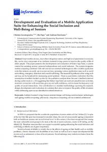
Figure 1.

Site index map, showing the locations of the three investigation sites: Aberg, Beberg, and Ceberg.

that the repository and canisters are successfully built to design specifications and that present-day climatic and geological conditions persist throughout the time period of interest (SKB, 1999b). One alternative scenario considers the impact of future earthquakes on a particular aspect of the repository. The earthquake Scenario (SKB, 1999b) is identical to the base case Scenario, with the difference that future earthquakes may impact the mechanical integrity of the canisters themselves or the backfill material surrounding them. The earthquake Scenario focuses on the possible damage to canisters due to the earthquake-induced movements of natural rock fractures that intersect them. In this scenario, a future earthquake occurs on a fault not directly intersecting the canister. Energy from this event produces slip on the fracture intersecting the canister. Based on pessimistic calculations for canister integrity, induced slips greater than 0.1 m are assumed to damage the canister (SKB, 1999b). There are several types of uncertainty that must be included in safety calculations. Conceptual uncertainties include uncertainties about fundamental physical processes and model uncertainties, which pertain to how physical processes are represented in numerical models (SKB, 1999b).

Data uncertainties, on the other hand, arise from incomplete knowledge about boundary conditions, material properties, and other model input (SKB, 1999b). The performance assessment of the repository under these differing types of uncertainty typically relies upon a stochastic approach. This involves the sampling of statistical distributions for model input data and for selection of scenarios that have been weighted as to their perceived likelihood of occurrence; the comparison of alternative numerical formulations to predict the outcome of the same physical processes; and the comparison of the impact of including different physical processes using the same numerical formulations. It is not always possible to represent all of the postulated physical processes in a numerical model, and similarly, it may not be possible to specify probability distributions for some input data or conditions. A common strategy is to bound the calculations, either by adopting conservative assumptions about the processes in order to simplify them or to adopt pessimistic values for the input data. It is important that model simplifications or bounding data values lead to conservative results. A conservative result is one in which the predicted harmful impact, in this case canister failure due to fracture slippage, occurs more often than had the simplification not been made or the full probability distribution for the data been used. One approach to estimating induced slip is to calibrate a probability distribution from field studies of induced slip (Coppersmith and Youngs, 2000). In this approach, the estimated induced slip is a probabilistic function of the distance from and the amount of slip on the primary rupture. However, no such field studies exist for Fennoscandia, nor would it be easy to obtain this data for paleoseismic events such as postglacial faulting where it is unclear which secondary ruptures are associated with a primary rupture. In lieu of such field studies, it is necessary to develop a method that does not rely upon a field data set of induced slips. Thus, the current study focuses on developing and assessing a process to determine this particular seismic hazard within the context of the Swedish program. Some of the model input data concerning future seismicity and the geological fracture pattern are based on preliminary, limited data or assumptions that should be reconsidered before the methodology is applied to evaluate a specific candidate site. These areas are noted.

Modeling Approach The estimation of induced slip requires the definition of certain conceptual models and the numerical implementation of these models. Figure 2 illustrates how the conceptual and numerical models are related. All models are fully three dimensional. The top line of this figure identifies the four conceptual models needed. The lineament and future earthquake models together define the number, location, and magnitude of future earthquakes, as well as the rupture geometry and

Distributed Slip on Fractures due to Future Earthquakes for Nuclear Waste Repository Performance Assessment

925

The canister model, in contrast, is entirely deterministic. A single canister layout is used for each site, although the layouts do differ among the three sites. Once these models have been established, they are translated into numerical models. The numerical simulation process shown in Figure 2 begins with the specification of the number of stochastic realizations of the future seismicity. A realization consists of a stochastic sample from the equation 具log(n(M))典 ⳱ 具Log(a)典 ⳮ 具b典 * M,

Figure 2.

Outline of modeling approach showing submodels and processes. Variables shown in 具典 indicate that the values are stochastically selected or generated. Shading of boxes indicates components of a submodel or process. Variables regarding earthquake rupture parameters are explained in the text.

fault movement. The canister layout and fractured rock models together define which canisters are intersected by fractures and the geometric and mechanical properties of those fractures. The fractured rock model describes the geometry of the natural fractures and their mechanical properties in the region surrounding the hypothetical repository. This model is stochastic because the pattern of natural fractures is generated through stochastic sampling of the probability distributions governing fracture location, size, orientation, and mechanical properties. The probability distributions for these parameters are derived from data measured or inferred for each site. The future earthquake model is likewise stochastic because the location, size, date, and other salient aspects of future seismicity are not known with little uncertainty. The conceptual model for the lineaments contains both deterministic and stochastic components. Smaller lineaments and lineaments that are presently obscured water or vegatation are not represented in lineament maps. Stochastic representation of these smaller or obscured lineaments supplements the mapped lineaments to form a combined stochastic-deterministic model.

(1)

where M is the earthquake magnitude; n(M) is the number of earthquakes of magnitude greater than or equal to M; a and b are parameters estimated from the earthquake catalog that together describe the ratio of large earthquakes to small earthquakes, and the spatial density of earthquakes; and the symbols 具典 are used to denote the expected value of the variable or function. The parameters a and b depend upon the time period of interest and the amount of area. Because these parameters are stochastic, the actual number of earthquakes for each magnitude class may differ among realizations. The greatest difference occurs for the largest magnitude classes. In some realizations, there may be an earthquake with ML ⬎7.0, while in others, there are none. Since the largest magnitude earthquakes produce the greatest slip, realizations containing earthquakes with large magnitudes may produce significantly more canister damage than those realizations that do not. Current seismicity in Fennoscandia appears to take place on existing faults expressed at the surface as lineaments (Stanfors and Ericsson, 1993; Saari, 2000). It is likely that earthquakes over the next 100,000 yr will also take place along existing crustal ruptures in Sweden given the highly fractured, blocky nature of the crust (Stephansson et al., 1979; Stanfors and Ericsson, 1993), which should readjust to loads imposed by block movements rather than through the creation of new ruptures. There are statistically robust relations between the geometry of an earthquake rupture zone, the slip on the surface, and the earthquake magnitude (Wells and Coppersmith, 1994). Some of the regression coefficients differ by fault type. These relations make it possible to infer the range of surface trace lengths of the rupture zone that would be expected for an earthquake of a specific magnitude or to predict the range of maximum displacements that would be expected as a function of magnitude. Thus, the magnitude of a future earthquake and the surface length of existing bedrock fractures lineaments constrain the location for each future earthquake in the model. The procedure for defining the relevant earthquake parameters for each future earthquake is based upon regression equations (Wells and Coppersmith, 1994) between magnitude and rupture width (RW), magnitude and surface rupture length (SRL), and magnitude and maximum rupture displacement (MD). These regressions have an associated probability distribution around the mean regression that is a func-

926 tion of the number of data points in the regression and the variance about the regression. The uncertainty in the regression is incorporated by making a Monte Carlo draw from the distribution around the variable of interest for the specified magnitude. First, a value for SRL is selected from the regression between SRL and magnitude for a specified magnitude. The selected SRL value is used to select lineament. The lineament segments in the lineament data base are searched randomly until one is found that is at least as long as the required SRL. This lineament then becomes the location of the earthquake, and the rupture zone’s surface trace is centered on the center of the selected lineament. The width of the rupture zone and the maximum displacement for this earthquake are also selected in a manner analogous to the SRL using the regressions between magnitude and rupture width, and between magnitude and maximum displacement. The fault type selected is that which maximizes the product of slip times rupture area, so as to produce the greatest induced slip on fractures intersecting canisters. The orientation of the rupture surface is based on the mean trend of the lineament; the dip is assumed to be vertical with some small randomly selected component of variability. Thus, the earthquake magnitude is used to assign a rupture length, width, and maximum displacement and to select a location in conjunction with the surface lineaments. The assignment of displacement to the rupture surface in the model is simplified but conservative. Displacement along an earthquake rupture surface in not uniform. Displacements are greatest at the location where the rupture initiates and diminish outward until they reach 0.0 at the tip line. However, the models assign the maximum displacement to the entire rupture surface, making it possible to ignore the spatial distribution of slip through a conservative assignment of the maximum slip to the entire rupture. In the algorithm adopted, the future earthquake is situated such that the center of the surface rupture trace coincides with the centroid of a suitable lineament trace. Earthquake ruptures are not necessarily centered on the centers of existing ruptures; in fact, classical seismic risk assessment presumes that epicenters are randomly located along the active fault or lineament. However, the effect of centering future earthquake rupture surfaces on centroids of existing lineaments is likely to be negligible. As shown in the Results of Calculations Section, it is only the large magnitude (ML ⬎5) earthquakes that have any probability of producing canister damage, and then only if they are within a few kilometers of the canisters. These larger earthquakes, numbering somewhere on the order of 20 or fewer for a 100,000-yr time period within a 100km circular region surrounding the repository, require surface ruptures on the order of kilometers to tens of kilometers. There are very few lineament segments that are substantially greater than the surface rupture lengths required by these key large earthquakes, which implies that the random assignment of the future earthquake to any acceptable portion of the lineament would still be constrained to a small interval


around the lineament segment centroids. This constraint along with the conservative assignment of slip to the entire rupture surface should reduce the impact to a negligible effect. Earthquakes also have a temporal pattern. Conventional earthquake hazard studies often calculate risk assuming a Poissonian distribution. While seismicity over a few decades may conform to a Poissonian distribution, it is an open question as to whether a Poissonian model adequately represents the temporal pattern of earthquakes over 100,000 yr, especially when the cyclical nature of glaciation is considered. In the current modeling process, the temporal pattern of future seismicity is assumed to be Poissonian. This means that the earthquakes occur at time intervals conforming to an exponential distribution, and that their magnitudes are independent (not correlated in time). We discuss the possible departure from a simple Poisson process in a following section. Accompanying each future seismicity realization is a realization of the natural fracture system, 具F典. This fracture realization is combined with the canister layout model (C) to generate a final fracture model consisting of only those fractures that intersect canisters (FC). The darker shaded portion of Figure 2 shows processes related to the generation of the realizations for future seismicity and fracturing. The lighter shaded interior portions of Figure 2 correspond to the calculations carried out for each future earthquake. A rectangle with a displacement field represents each future earthquake (R) in the numerical model, which requires the specification of the rupture location, geometry, and displacement. These parameters are stochastic in that they are generated through Monte Carlo sampling of the regression relations that relate earthquake magnitude to these parameters. Locations are also stochastic, as they are randomly selected from the lineaments with only the restriction that the lineament segment trace length be at least as long as the randomly selected SRL for the earthquake. Once the specific rupture geometry and displacement field are defined for the earthquake, they are combined into a single numerical model with the fractures that intersect the canisters. The model produces an estimate of slip on each fracture that intersects a canister. The cumulative slip on each fracture is determined by the vector addition of the slips for each earthquake. After all of the earthquakes for a particular seismic realization have been simulated, the number of canisters intersected by fractures experiencing slips greater than the threshold value of 0.1 m is tabulated. After all the seismic realizations have been completed, several summary statistics quantify canister failure due to induced slips.

Parameter Values and Key Assumptions Modeling is a process of simplifying complex physical processes and data variability to simpler forms through assumptions. This section describes the input parameter values


and some of the key assumptions that were used in order to apply the method to the three generic sites. Some of the values and the assumptions point out where future work may be necessary to reduce the uncertainty of the results. Future Seismicity There are four considerations for development of a model for future seismicity: (1) the role of tectonic and glacial unloading processes in the generation of the current earthquake catalog, as well as in future earthquakes, throughout the 100,000-yr performance period; (2) the extrapolation of the current catalog spanning about 100 yr that contains earthquakes with magnitudes ML rarely exceeding 4.5 to forecast large earthquakes over a vastly larger time frame; (3) the treatment of foreshocks and aftershocks; and (4) the location of future earthquakes. Each of these is discussed in turn. Tectonic Versus Glacial Processes. Current tectonic conditions and the state of stress in the Baltic Shield have been stable over the past 2 million yr, (Muir-Wood, 1995). This area has also witnessed shorter-term loading due to glaciation and deglaciation. It is anticipated that another glacial cycle will occur within the next 100,000 yr in Fennoscandia (SKB, 1999a). It is not clear what state of stress will occur under the ice cover and its margins, nor how long it might take for the tectonic stress field to recover after deglaciation. Scarps in Sweden and elsewhere in Fennoscandia has been interpreted by some investigators (Lukashov, 1995; Arvidsson, 1996; Johnston, 1996) as single rupture events resulting from postglacial faulting caused by deglaciation several thousand years ago. Based upon the surface trace length of these scarps and other field evidence, these postglacial earthquakes could have been as large as MW 8.2. There also still exists some uncertainty as to whether present-day earthquakes in Sweden are tectonic in origin, resulting from ridge push in the Atlantic (e.g., Slunga, 1991), or whether they are largely due to ongoing glacial rebound (e.g., Muir-Wood, 1993). Saari’s (2000) estimate of the energy release required by the seismic activity in Fennoscandia led him to conclude that the majority of the energy comes from North Atlantic ridge push, whereas rebound and deglaciation serve primarily as mechanisms for releasing this stored energy. The possibility that there are two sources for earthquakes is important for correctly extrapolating the current earthquake catalog. For example, if the mechanism of ridge push is producing current seismic activity, then the recent instrumental and historical earthquakes form a reasonable basis for forecasting tectonically induced activity over the next 100,000 yr, notwithstanding the previously mentioned problem of extrapolating a and b parameters from small events to large events. This also implies that seismicity due to glacial unloading would not be captured at all in the current a- and b-values. Alternatively, if current seismicity reflects glacial rebound, then future activity will decrease until the end of the next glacial cycle at which time it will in-

927

crease. Thus an extrapolation of the current seismic catalog would overestimate the expected magnitude/frequency of earthquakes prior to the next glaciation and underestimate the number of large earthquakes during deglaciation. Saari (2000) has suggested that an appropriate model for Finland would be to extrapolate the current seismic activity to the 100,000-yr time frame but to restrict the larger earthquakes to the end of this time period. If this model were followed for Sweden, then the large, possibly damaging future earthquakes would occur only at the end of the performance period, but they would not affect the overall damage probabilities. However, an actual repository’s performance would be better the later a damaging event occurred, since radioactive decay reduces the impact of the damage with time. Thus, allowing large earthquakes to occur at any time is a conservative assumption. The issues regarding future seismicity in Sweden have not been unambiguously resolved. For the purposes of this study, the a- and b-values reflecting recent seismicity are assumed to be constant and representative throughout the 100,000-yr time frame. Temporal and Magnitude Extrapolation. There is uncertainty in using the seismicity in Sweden of the past 100 yr to model seismicity for the next 100,000 yr, independent of whether glacial or tectonic processes are responsible. The current earthquake catalog contains historically and instrumentally recorded earthquakes. Seismicity has been low in Sweden both in magnitude and in numbers or earthquakes. The largest event during this time period had a magnitude (ML) of approximately 5.0 (Slunga, 1985, 1991). The small number of earthquakes and their small magnitudes means that the estimation of a and b contain some estimation variance, and perhaps more importantly, make extrapolation of the small magnitude regression relations to large magnitude earthquakes uncertain both for mathematical and physical reasons. The physical mechanisms that lead to large magnitude earthquakes may differ from those that produce small or moderate magnitude earthquakes. If this is the case, then even perfect knowledge of the smaller earthquakes may not accurately predict the number of large earthquakes in the future. Seismic hazard studies often estimate a characteristic maximum magnitude earthquake, based on seismic strain release or other considerations. However, since the instrumental and historical catalog for Fennoscandia does not include possible postglacial earthquakes, which would have different and probably higher strain-release rates, any calculation of a characteristic maximum magnitude from the current catalog based on energy release rates is probably an underestimate. Saari (2000) has attempted to estimate a maximum characteristic earthquake for four seismotectonic regions in Finland, which have similar geology and seismic settings as do the Swedish sites. Saari (2000) estimated the maximum earthquake by projecting the current strain-release rates over the next 100,000 yr and assuming that all of the

928 energy is released by a single earthquake at the end of 100,000 yr. He calculated maximum values of ML from 7.4 to 8.2. Earthquakes of magnitude ML 7.5 or greater have probabilities of less than 1.0 for the seismotectonic regions encompassing the three Swedish sites. Although maximum characteristic earthquakes have not been calculated for the seismotectonic regions in Sweden, the calculations for Finland in somewhat similar regions indicate a maximum earthquake of ML ⱖ7.4, which are very low probability events in Sweden. Thus, not establishing a maximum magnitude for the Swedish simulations would probably play little role in eliminating a low-probability large earthquake, and, in any event, the lack of magnitude truncation is conservative. There are also mathematical uncertainties in extrapolating large earthquake frequencies from a catalog only containing small magnitude earthquakes. The size of the confidence intervals around a function estimated through regression are narrowest at the mean of the independent variable and become wider to either side (for example, see regressions of Wells and Coppersmith, [1994]). The width depends in part on the variance. The mean of the historical/ instrumental catalog is toward the smaller magnitudes. This implies that the confidence intervals for the larger (ML ⬎5) earthquakes will have much larger confidence intervals and hence much higher uncertainty. The resolution of these issues is beyond the scope of the current study, which focuses on methodology. Clearly these considerations must be satisfactorily addressed in the future to evaluate an actual candidate site. For the purposes of this study, however, it is assumed that the current a- and b-values calculated from historical and instrumental events could be extrapolated to earthquakes of larger magnitude, with no upper magnitude truncation. Kijko et al. (1993) developed the current estimates of the parameters governing the magnitude/frequency relations of earthquakes in Sweden. They divided Sweden into a southern and northern zone along the 60⬚ N parallel (Fig. 3). Within southern Sweden, there is a subregion of increased seismicity termed the Lake Va¨nern subregion. There is also a region of higher seismicity along the coast of the Gulf of Bothnia. Table 1 shows the seismic hazard parameters for these two regions and their subregions. The minimum magnitude earthquake used to estimate parameters was ML 1.9, with an upper maximum magnitude varying by subregion (MM 4.8 for southern Sweden; MM 4.3 for northern Sweden). Lower b-values for the southern region indicate that the proportion of large earthquakes to small earthquakes is greater in the south than in the north. This is consistent with the observation by Skordas and Kulhańek (1992) that northern Sweden “has a pronounced earthquake activity but practically all seismic energy is released through a number of relatively weak shocks” (p. 583). Aberg and Beberg are both south of 60⬚ N; thus the seismicity data for southern Sweden is the most relevant for


Figure 3. Earthquake epicenter distribution in Sweden for the period 1375–1989, including seismic hazard subregions.

predicting future earthquakes at these two sites. However, the southern Sweden catalog is heavily influenced by seismic activity within the Lake Va¨nern subregion that is far from either site. A realistic estimate of future earthquake frequencies at Aberg and Beberg should compensate in some way for the fact that these sites will be much less affected by activity in the Lake Va¨nern subregion than the averaged parameters for all of southern Sweden would indicate. It is difficult to make reliable parameter estimates directly due to the small number of earthquakes that have been recorded outside of the Lake Va¨nern subregion in southern Sweden. It is not valid to remove the earthquakes predicted for the Lake Va¨nern subregion from the total predicted for all of southern Sweden for obvious mathematical reasons: Figure 4 shows the predicted earthquake activity for each of the four seismic regions extrapolated for a 100,000-yr time period and also to earthquakes above and below the minimum magnitudes used in the parameter estimation. The curve representing the activity obtained by removing the number of earthquakes (labeled as “Subtracted Data” in Fig. 4) predicted for the Lake Va¨nern subregion from the southern Sweden region is shown on this plot. The predicted number becomes negative for magnitudes approaching 5.0. This problem is due to extrapolation from small magnitudes to larger ones and to the magnitude of uncertainties in the regression parameters. To try to compensate for these errors, the portion of this curve that corresponds to the small magnitude earthquakes was extrapolated and then adjusted to correspond to the area of a 100-km radius circle. Since this is the portion where there is measured data, the resulting a and b parameters might be a closer approximation of the future magnitude/frequency in the Aberg or Beberg regions.

929


Table 1 Seismic Hazard Parameters for Sweden* Area

Southern Sweden Lake Va¨nern Northern Sweden Coast of Gulf of Bothnia Adjusted Southern Sweden†

b

a

k2.4

mmax

N

1.04 Ⳳ 0.05 0.98 Ⳳ 0.06 1.35 Ⳳ 0.06 1.26 Ⳳ 0.06 1.11

564 292 6430 2536 272

1.8 Ⳳ 0.2 1.3 Ⳳ 0.2 3.7 Ⳳ 0.3 2.4 Ⳳ 0.2 0.6

4.9 Ⳳ 0.5 4.9 Ⳳ 0.5 4.3 Ⳳ 0.5 4.3 Ⳳ 0.5

135 104 241 164

*k2.4 is the number of annually expected earthquakes with magnitude 2.4 or larger and reflects the minimum magnitude threshold for the instrumental catalog for the interval 1951–1989. mmax is the maximum expected magnitude during a time span equal to that of the catalog, and N is the total number of earthquakes expected in that time span above the threshold magnitude (ML 2.4). The value for a is derived from the other parameters. The uncertainty in the parameters is the standard error. † Parameters estimated via regression as described in text.

Figure 4 shows the result in the curve labeled “Extrapolation.” The parameter values estimated for this line are a ⳱ 126.53 and b ⳱ 1.113. They are referred to as the “adjusted southern Sweden” seismic parameters. For completeness, forecasts of future seismicity for Aberg and Beberg used both the southern Sweden (including Lake Va¨nern) and adjusted southern Sweden a and b parameter values. Forecasts for Beberg also included two additional scenarios. Because Beberg is near the 60⬚ N parallel, future seismicity for this site might also reflect seismicity in the northern Sweden and Gulf of Bothnia catalogs. Future seismicity for Ceberg simulations was forecast from only the northern Sweden and Gulf of Bothnia parameters. Aftershocks and Foreshocks. The earthquake catalog used by Kijko et al. (1993) in the previous section does not include aftershocks and foreshocks. These events can often be quite large for large main events. They also do not occur at random in time or space, but are closely associated in time and coincident in space. Extrapolation of the a- and b-values does not account for them. The method outlined in this study is sufficiently flexible that temporal and spatial models for foreshocks or aftershocks could easily be incorporated. The calculations reported in this study do not include them, however.

Figure 4.

Number of earthquakes expected over a 100,000-yr time period for the seismic regions in Sweden. Subtracted data is calculated by subtracting the earthquakes from the Lake Va¨nern subregion from the southern Sweden region. The curve labeled extrapolation is calculated by fitting a line to the small magnitude (ML ⬍3) portion of the subtracted data curve.

Table 2 Data Sources for Scaling Analyses

Location of Future Earthquakes. The bedrock in Sweden is quite old, having largely formed through a series of orogenies between 1.5 and 3.5 billion yr ago (Muir-Wood, 1993; Juhlin et al., 1998). The Caledonian orogeny (⬃0.4 billion yr) is the most recent major tectonic event to influence Swedish bedrock structure. As a result of these orogenies, the rock exhibits well-developed systems of fractures and fracture zones that might serve as locations for future earthquakes. Field studies of past earthquakes suggest that they took place as reactivations of existing fractures (Stanfors and Ericsson, 1993). As described previously, the magnitude of the future earthquake and the length of lineament segments constrains the location of the rupture. Table 2 shows the source for these lineament maps.

Source

Scale

Aberg Tireń and Beckholmen (1990) Tireń et al. (1987) Tireń et al. (1987) Nisca and Triumf (1989)

1:1,000,000 1:250,000 1:150,000 1:7,000

Beberg Bergman et al. (1996) Bergman et al. (1996) Ahlbom and Tireń (1991) Ahlbom and Tireń (1991) Andersson et al. (1991)

1:400,000 (west) 1:400,000 (east) 1:87,000 1:20,000 1:20

Ceberg Hermanson et al. (1997) Hermanson et al. (1997)

1:200,000 1:20,000

930 Lineament maps represent data at or above a certain resolution scale; there may be many potential lineaments that could host smaller earthquakes that do not appear in the lineament maps. Moreover, water, vegetation, and urban development often cover up lineaments. Both of these issues have been addressed in the current approach. It has been assumed that the lineaments below detection resolution have the same orientations as the larger lineaments. It has also been assumed that obscured lineaments are statistically the same as those that can be observed. Therefore, earthquakes below a magnitude corresponding to the smallest traces in the lineament maps are not situated on an existing lineament but rather are located at random anywhere within the 100-km circle. The strike of the rupture plane is taken from a Monte Carlo sample of the lineament trends in the lineament database. If a future earthquake is large enough to be situated on an identified lineament, then an additional operation is carried out to help compensate for censoring effects. The major censoring feature in the three generic sites, which lie largely along the coastline, is the sea. Water covers up about half of the area of interest. To compensate, the location of each earthquake event situated on an existing lineament can be reflected 180⬚ through the center of the repository with a 50% probability. This procedure assumes that the lineaments underneath the sea are statistically the same as those on land. This is a reasonable assumption for the seismic provinces south of 60⬚ N, given the spatial homogeneity of seismic activity in these areas. However, Figure 3 shows that the spatial pattern of earthquake epicenters north of 60⬚ N is not uniform. Rather, they appear to be clustered along the coastline. This spatially inhomogeneous distribution potentially impacts the Ceberg site calculations. Ceberg is several tens of kilometers southwest of the city of Umea˚ (Fig. 1) and about 10 km inland from the coast. The site lies about 10 km from the nearest instrumentally or historically recorded earthquake shown in Figure 3, putting it outside the belt of higher seismic activity. The activity parameters for the Gulf of Bothnia subregion average seismic activity over both the belt of higher seismicity and the areas of lower seismicity outside of this belt. Analysis of the earthquakes that produced canister damage in the numerical simulations at Ceberg (see Canister Failure Proportion Probabilities) show that earthquakes occurring on lineaments farther than a few kilometers do not produce damage. Since Ceberg lies in a region of very low seismic activity in the critical few kilometers surrounding the site, the use of averaged parameters probably overestimates the magnitude of seismic activity in this local region and is thus conservative. Other future sites in the Gulf of Bothnia subregion may be situated in regions of higher activity than Ceberg. In these cases, it may be necessary to revise the seismic parameters to reflect the spatial inhomogeneity of the recent earthquake activity, as using the spatially averaged results may not prove conservative.


Geological Fracture Model Statistical models for fracturing at the three generic sites were prepared from a variety of different data. Aberg, lo¨ spo¨ Island in southern Sweden, is the site of an cated at A extensive underground laboratory that includes shafts and tunnels to a depth of 500 m. Beberg, near the coastline in central Sweden, is near Lake Finnsjo¨n, whereas Ceberg, further inland in northern Sweden, is near the town of Gidea˚. The level of knowledge about fractures on the order of a few tens of meters or less differs among the three generic sites due to differing levels of site investigations. Aberg has the greatest variety and quantity of geological information due to the underground research laboratory at this site. There are no underground research facilities at either Beberg or Ceberg. The smallest-scale fracture data at these two sites comes from surface mapping of outcrops and trenches. It is not possible to determine the location, orientation, size, and mechanical properties of every fracture that might potentially intersect a canister hole. Even with exploratory drilling, geophysical imaging, and detailed surface mapping, most fractures will not be detected, even though they may affect repository performance. Moreover, data gathered from any source is limited by the minimum and maximum fracture size it can reliably detect. Typically, these scale ranges do not overlap, leaving large gaps in scale between them. Both of these factors contribute to uncertainty in the fracture model. Stochastic fracture modeling methods described in a later section make it possible to incorporate the uncertainty due to small number of measurements relative to the entire fracture population. Analysis of fracture geometry and intensity at several different scales makes it possible to generate fractures at scales where little or no data is available and thus to resolve the scaling issue. Scaling analysis involves comparing fracture orientations, fracture intensity, and trace length distributions from all scales. Fracture intensity in this context is defined (Dershowitz and Herda, 1992) as the ratio of measured fracture trace length to rock surface area (P21) or as the ratio of fracture surface area to rock volume (P32). It is important to perform scaling analyses on each fracture set separately because the mechanical processes that lead to the formation of different fracture sets could easily produce different characteristic fracture sizes and intensities (Barton, 1995). The values derived for each site are summarized in Table 3. La Pointe et al. (1999) provided details concerning these calculations and the sources for the data. Details concerning the data itself are presented by SKB (1999b). The results for Beberg are presented in Figure 5 and Figure 6 to illustrate the process. Fracture lineament maps were analyzed at three different scales. The lineament map at the 1:400,000 scale was split into an east and west portion, pertaining to a visually significant difference in lineament intensity. Beberg is located in the western half of this map, and thus the analyses for this western portion are more relevant.


931

Table 3 Scaling Exponents for Tracelength and Spatial Intensity Map

No. of Sets

Set Orients

D (tracelength)

Aberg 1:2,000,000 1:250,000 1:150,000 1:7,000

4 3 3 4

EW, NE, NS, NW NS, NW, EW NS, NW, NE NS, NE, NW, EW

D ⳱ 1.66 D ⳱ 1.56 D ⳱ 1.52 D ⳱ 1.60

Db ⳱ Db ⳱ Db ⳱ Db ⳱

1.60 1.59 1.71 1.61

Beberg 1:400,000 west 1:400,000 east 1:87,000 1:20,000 1:20

2 3 3 3 1

N, ENE N, NE, WNW NNE, NW, NNW NNE, NW, NNW —

D ⳱ 1.7 D ⳱ 1.85 Too few data points D ⳱ 1.7 D ⳱ 1.8

Db ⳱ Db ⳱ Db ⳱ Db ⳱ Db ⳱

1.8 1.8 1.8 1.8 1.25

Ceberg 1:200,000 1:20,000

2 2

NS, EW EW, NESW

D ⳱ 1.85 D ⳱ 1.95

Figure 5. Rose diagrams of lineament trends for Beberg for maps at different scales. (a) 1:400,000, east half; (b) 1:400,000, west half; (c) 1:87,000; (d) 1:20,000.

The first step is to determine if the same fracture sets are present at the different scales. Figure 5 shows the orientation rosettes of lineament traces for the different maps. In all cases, a north–south set is prominent. In the 1:20,000 scale map, which has the smallest lineaments and is thus closest to the scale of fractures that intersect canisters, there are two other prominent sets, and perhaps one or two less prominent sets. The other two prominent sets are a northeast set and a northwest set. Both of these sets are clearly visible on the 1:87,000 scale map. The northwest set is also clearly evident on the 1:400,000 scale map, although it is dominated to a greater extent by the north–south set on the west half of the 1:400,000 map. The northeast set is also evident on

D (box)

D ⳱ 1.7 D ⳱ 1.7

the 1:400,000 map but is not as important relative to the north–south set as it is on the smaller-scale maps. In all of the maps, there is an indication of an additional minor set that trends east–west. The minor north-northwest set evident in the 1:20,000 scale map is not obviously present in the other maps and may only appear as a distinct set in the 1:20,000 map due to the smaller amount of data underlying that rosette. Thus, the rosette suggests that there are four sets of lineament orientations that are present at all three scales, although the relative intensity of each set may vary among the scales. The statistical model for fracture orientations for each site was calculated in different ways according to the data available. At Aberg, previous work by Follin and Herman¨ spo¨ son (1996) on fracture orientations measured in the A underground research laboratory provide sufficient information to calculate orientation distribution statistics for each fracture set. For Beberg and Ceberg, sufficient threedimensional fracture orientation data was not available. At these sites, the mean orientation of fractures was assumed to be vertical with the orientation dispersion values given in Table 4. The strike of the fractures conformed to orientation models estimated from the trace (lineament) data. The determination as to whether trace lengths at each map scale reflect a doubly truncated sample from a single parent distribution requires the computation of trace-length size distribution for each dataset and trace orientation set. A mathematically convenient way to analyze the tracelength distribution is to compute the complementary cumulative density function (CCDF) for each set and data source. The CCDF is the probability that X is greater than x, or P(X ⬎ x). Many field studies (e.g., Gudmundsson, 1987; Villemin and Sunwoo, 1987; Scholz et al., 1993) have demonstrated that fracture trace lengths conform to a power law, and there are various mechanical and physical reasons why this should be so (Turcotte, 1992; Bak and Chen, 1995; Scholz, 1995).

932


Figure 6.

Trace length scaling behavior for individual sets, Beberg site.

Figure 6 shows the plots of the CCDF for individual fracture sets at Beberg. The departure from linearity at small lengths is a sampling bias, as described by La Pointe et al. (1999). Table 3 shows the calculated values for the scaling exponent, D, for all fracture sets and data sources. This table and the accompanying plots show that the trace length appears to scale according to a power law at all scales and that exponent is reasonably consistent for the individual sets across all scales. The next step is to combine with individual CCDFs for each set in order to estimate the parent population parameters. Figure 7 shows the result obtained for Beberg normalized for the map area as described by Castaing et al. (1996). The alignment of data from different scales indicates that the trace-length distributions measured at different scales do appear to be doubly truncated samples drawn from a single parent power-law distribution. Results for the other two sites were also aligned. Table 3 summarizes the results for the other sites.

The spatial pattern of fracturing concerns whether fractures are located at random, as if their centers were located according to a Poisson process, or whether there is some structure to their locations. Whether this structure changes at different scales is of particular interest. Together with fracture intensity, the spatial pattern of fracturing also influences canister-fracture intersections. Barton and Larsen (1985) first used the fractal box dimension of fracture trace patterns in order to assess their scaling behavior. If all the different scale maps for the same fracture set show a power-law behavior characterized by the same scaling exponent, or box dimension, then it is reasonable to assume that the fracture intensity scales according to a simple power-law function. The consistency of the dimension values in a region strongly supports the decision to treat the fractures as a single population over the scale of the maps analyzed. Figure 8 shows an example of box dimension calculation for the Beberg data. Each curve plotted in the figure can


933

Table 4 DFN Model Parameters Parameter

Value

Aberg Set 1 Orientation (Mean pole trend, plunge, dispersion) Intensity (P32)

58.7, 1.8, j ⳱ 13.37 Fisher model 1.4333

Set 2 Orientation (Mean pole trend, plunge, dispersion) Intensity (P32)

334.2, 5.6, j ⳱ 7.82 Fisher model 0.7509

Set 3 Orientation (Mean pole trend, plunge, dispersion) Intensity (P32) Size

Mechanical Properties Spatial Model

71.7, 85.5, j ⳱ 11.92 Fisher model 0.7807 Power Law, D ⳱ 2.6 X0 ⳱ 0.1 m Min ⳱ 3 m, Max ⳱ 50 m Frictionless, cohesionless Poissonian

Beberg Set 1 Orientation (mean pole trend, plunge, dispersion) Intensity (P32) Set 2 Orientation (mean pole trend, plunge, dispersion) Intensity (P32) Set 3 Orientation (mean pole trend, plunge, dispersion) Intensity (P32) All Sets Size Mechanical Properties Spatial Model

125.0, 0.0, j ⳱ 75 0.02 215.0, 0.0, j ⳱ 50 0.04 85.0, 0.0, j ⳱ 30 0.04 Power Law, D ⳱ 2.7, x0 ⳱ 10 m Frictionless, cohesionless Poissonian

Ceberg Set 1 Orientation (mean pole trend, plunge, dispersion) Intensity (P32) Set 2 Orientation (mean pole trend, plunge, dispersion) Intensity (P32) All Sets Size Mechanical Properties Spatial Model

175.0, 0.0, j ⳱ 50 0.08 135.0, 0.0, j ⳱ 50 0.04 Power Law, D ⳱ 2.85, x0 ⳱ 10 m Frictionless, cohesionless Poissonian

Figure 7. Cumulative trace length distributions by sets at different scales, Beberg site.

be broken into two linear segments. The more shallowly dipping portion has a slope of approximately 1.0 and is an artifact of allowing box sizes to become too small (Barton, 1995). The steeper portion of each curve is not biased by box size and represents the true box dimension of the data. Nonlinear regression of this more steeply dipping portion of each curve yields box consistently around 1.8, with the exception of the traces on the 1:20 map, which is a very sparse dataset that makes it difficult to robustly determine the fractal dimension. Box dimension graphs for the other site also showed a power law-relation. Table 3 summarizes mean box dimensions for the trace maps. A box dimension close to 2.0 implies that although the trace intensity may have fractal characteristics, a spatially random (Poissonian) process might also approximate the pattern. Treating the fractures as Poissonian when the true dimension is 1.8 produces a negligible impact on the number of canisters intersected by fractures and is a much simpler numerical process and thus was used for the fracture models in this study. The box dimension describes the scaling behavior of fracture spatial distribution but does not quantify the absolute value of fracture intensity. The desired intensity parameter for modeling is the fracture surface area per unit volume of rock, or P32. This parameter is not directly measured but can be calculated from other measured data. The P32 calculation for Beberg illustrates how this is done. The CCDF for fracture traces on the 1:20,000 map (Fig. 6) begins to depart from linearity for trace lengths less than 300 m. If all traces shorter than 300 m are removed from the 1:20,000 trace map, the trace-length intensity (trace length per unit area, or P21) is 0.007 mⳮ1. This value of P21 is used to calculate P32. The calculation involves a numerical simulation of fractures represented as polygons in a volume. The polygons have an orientation distribution and a size distribution corresponding to the orientation and size distributions for each fracture set shown in Table 4. Next, a horizontal plane is placed into the simulation. Some of the

934


Figure 8.

Box dimension calculations for fracture sets at Beberg.

fractures in the simulation intersect this plane, producing traces on the plane. The sum of the fracture trace length per unit area in the simulation plane is compared to the value determined from the lineament map. Values of P32 in the simulation are adjusted until the values of P21 in the simulation match the value determined from the lineaments. The simulations for Beberg indicated that a fracture area per volume intensity (P32) of 0.1 mⳮ1 produced a P21 equal to 0.007 mⳮ1 in the 2-km (the maximum trace length on the map) to 300-m size range. The fracture intensity is partitioned to the three sets identified in the rosette diagrams. This procedure was also carried out at Aberg and Ceberg. Table 4 summarizes the complete set of statistical parameters used to define the geometry and mechanical properties of fracturing over all scales of interest for each of the three sites. All three sites have similar fracture trace-length statistics and spatial patterns. The main difference is that the fracture intensity for Aberg is higher than for Beberg or Ceberg. This suggests that more fractures would intersect canisters at Aberg than at Beberg or Ceberg. Higher intersection probabilities lead to higher canister failure probabilities, all other factors being equal. Canister Layouts The geometry of the canister layouts is site specific. Details of the geometry for each site are described by La Pointe et al. (1999). In general, the canisters are emplaced in vertical holes 7.8 m high and spaced at 6-m intervals. Each site contains on the order of 4000 canister holes. Not all of the canister holes were used in the numerical simulations. In order to reduce the computational effort for assessment of the methodology, 970 randomly selected canister holes were used for the Aberg model, and 700 holes were used for the other two sites. This represents about 25% of the entire number of canisters. Simulations (La Pointe et al., 1999) have shown that the percentage of canisters intersected by fractures in this reduced set is statistically identical to the intersection percentage using the entire canister set. Numerical Model Implementation Simplifications and Conservativeness. The physical processes thought to occur when an earthquake induces slip on

a fracture must be simplified for numerical calculations. Fractures are three-dimensional ruptures in the rock with variable geometrical and mechanical properties. Fractures often have surfaces in contact with one another and may have some cohesion that will resist sliding forces due to cementation or other causes. The rheology of fractured rock is complex. Depending upon the loading conditions and the mineralogy and texture of the rock, it can exhibit responses characteristic of an elastic, viscous, plastic material or some combination of these. Under sufficient stress, fractures both deform and propagate. The rupture process during an earthquake is likewise complex. It is not instantaneous: the rupture nucleates in a local area and then propagates. The displacement field is not uniform over the surface (Wheeler, 1989). Moreover, energy emitted by the earthquake is propagated dynamically. There are no existing numerical tools that can simulate all of these physical processes in three dimensions concurrently. The numerical modeling simplifies some of the physical processes in order to obtain a computationally feasible solution. The next sections describe these simplifications and their conservativeness. The numerical implementation simplifies fracturing in several ways. First, fractures are idealized as frictionless, cohesionless planar polygons. The polygons are generated according to statistical distributions for size, location, and other parameters based upon the geology of each candidate site, as in Table 4. Such a numerical representation (Fig. 9) is called a discrete fracture network (DFN) model (Dershowitz and La Pointe, 1994). DFN models have been widely used in flow and transport calculations for fractured rock (Dershowitz et al., 1992; Swaby and Rawnsley, 1996), as well as for civil engineering (Dershowitz et al., 1991) and mining (Kleine et al., 1997) purposes. The assumption that fractures have no cohesion or surface friction is conservative, because both cohesion and friction will resist sliding. There is also some evidence to suggest that the assumption of no friction may actually be a realistic representation of fracture behavior under dynamic loads. Miller et al. (1990) showed that fractures behaved as if they were frictionless throughout dynamic loading, even


935

Figure 9. A discrete fracture network (DFN) model representation of a fractured rock mass. The top perspective view shows the 3D DFN model in which fractures are represented as polygons. The orientation, size, intensity, and mechanical properties of the fractures are controlled in these simulations by geological variables such as strain, rock type, curvature, or other factors. The plan view shows square cells with different shading levels that reflect relative fracture intensity. Orientations are controlled by the principal directions of strain. The inset shows three hypothetical canisters emplaced in the DFN model. The fractures that intersect canisters are retained for earthquake simulations using Poly3D.

when large normal stresses acted on the fracture. The representation of fractures as regular n-sided planar polygons could potentially impact canister intersection probability. Recent studies (Dershowitz et al., 2000) have shown, however, that this representation does not compromise accurate predictions of fracture intersection intensity. Secondly, fractures in the model only deform in response to loads; they do not propagate. In reality, when loads on a fracture exceed a threshold, stress concentrations at fracture edges increase to the point that fracture propagation occurs, and further slip is greatly reduced or ceases altogether. The neglect of propagation is a conservative assumption since it diverts energy that would have gone into fracture propagation into normal and shear displacement. It also places no upper limit on the amount of slip a fracture may experience. The conservativeness of neglecting friction, cohesion, and propagation has been explored by La Pointe et al. (2000) and has been found to produce slips that may be several orders of magnitude more conservative than if these physical mechanisms had been included in the numerical simulations. The other simplifications concern the transmission of energy from the earthquake rupture to the fracture. The modeling assumes that the rock is a linear elastic material and that the earthquake transmits energy as a static process. To the authors’ knowledge, there currently exist no codes that are capable of simulating the dynamic propagation of energy

through a material containing thousands of fractures represented as finite surfaces with general orientations in three dimensions. Instead, induced slip is modeled as a static process using the code Poly3D (Thomas, 1993). Poly3D is a three-dimensional linear elastic fracture mechanics code that uses a displacement-discontinuity formulation. The assumption of linear elasticity instead of a more complex rheology is conservative in that the energy imparted by the earthquake is applied to the fracture and is not dissipated by nonbrittle rock deformation or by other fractures. Each fracture in the model responds to the earthquake as if it were the only fracture in the model; shielding effects by other fractures do not occur. La Pointe et al. (2000) also investigated the shielding effects and found them to be conservative but not as important as neglecting fracture cohesion, friction, and propagation. Pollard and Segall (1987) presented field evidence to show that the normal displacement on dikes matches the displacement predicted from the linear elastic fracture mechanics solution, so the assumption of linear elasticity may be useful. On the other hand, dikes do not form through a dynamic process like earthquakes. Dynamic loading can produce locally higher energy density than a static elastic loading. This means that the energy available for deforming or propagating fractures may be higher than it would be for a static process. However, a dynamic process propagates waves in particular directions, so that not all of the rock in the vicinity

936


of the rupture is equally impacted. Also, common geological features such as fluid-filled fractures can reduce the effective transmission of these waves. This suggests that while a static solution might underestimate the energy available for fracture deformation in some locations, it might overestimate the energy in others. Another factor is that above a certain energy threshold, fractures will utilize some or most of the energy to propagate an existing fracture rather than focus all of the energy into elastic deformation, thereby reducing the incremental amount of slip associated with the additional energy. Recent fieldwork reported by Coppersmith and Youngs (2000) provides insight into the validity of calculating induced slip through a static process. They examined field data concerning the largest displacement found on an induced rupture and the largest displacement found for the principal rupture for normal faulting earthquakes in the Basin and Range province of the western United States. These earthquakes have magnitudes varying from 5 to nearly 8. Their compilations show that induced slip in the footwall of these normal faults is much less extensive than in the hanging wall. Data from five earthquakes shows only one instance of induced slip in the footwall, at about a distance of 1 km from the primary rupture. On the other hand, there were about 15 fractures exhibiting induced slip in the hanging wall. These fractures varied in distance from the primary rupture from a few hundred meters to a maximum of 13 km, with most of the fractures being within 5 km. The ratio of maximum induced slip to maximum rupture slip varied from a maximum value of 0.3 to a minimum of less than 0.1. Coppersmith and Youngs (2000) also plotted graphs showing the probability of induced slip as a function of distance. Their data shows that nearly all of the induced slip in the footwall occurs on fractures within about 7 km of the primary rupture and within 15 km of the primary rupture in the hanging wall. The data also shows that no induced fracture displacements were found for a number of locations surrounding the primary rupture. The results of the static simulation can be compared to these results in several ways. Poly3D was used to conduct a series of simulations in which the moment magnitude of the earthquake, its distance from a single fracture, and the relative position and orientation of the primary rupture and target fracture were varied through the ranges shown in Table

5. The maximum induced slip for all possible combinations of relative orientation and position for a 1-km target fracture size was tabulated as a function of earthquake moment magnitude and distance. Figure 10 shows the maximum induced slip found for the various combinations of relative orientation and position. The result is a continuous function given by log10 (max. induced slip) ⳱ 0.9Mw ⳮ 1.1log10 (distance) ⳮ 3.6

(2)

Or, using the relation between maximum displacement and magnitude reported by Wells and Coppersmith (1994): log10(max. induced slip) ⳱ log10 (primary rupture displacement) ⳮ 1.1log10 (distance) Ⳮ 2.7

(3)

These equations are specifically for a 1-km target fracture.

Figure 10. Maximum induced slip as a function of magnitude and distance.

Table 5 Parameter Ranges Used in Sensitivity Analyses Parameter

Range

No. of Steps Initial

No. of Steps Detailed

Parameter Varied in Detailed Runs

Earthquake Magnitude Distance Fracture size Azimuth Fracture orientation (Pole trend and plunge)

4–8 10 m–100 km 1 m–1000 km 0⬚–90⬚ both 0⬚–90⬚

7 11 4 5 7

— 21 — 7 49

— Azimuth — Distance and fracture orientation Azimuth


For the assumption of linear elasticity, the induced displacement is proportional to the radius (Pollard and Segall, 1987). Thus the results for the 1-km fracture can be easily adjusted for a fracture of any specified size. Figure 11 shows the ratio of maximum induced slip to maximum slip on the primary rupture as a function of distance based on equation (3) for three different fracture sizes. The gamma distribution with shape parameter 2.5 used by Coppersmith and Youngs (2000) to fit the empirical field data is also shown. Figure 11 shows that Poly3D simulations predict more induced slip for a 3-km fracture than was found in the hanging wall for the five field cases. The simulations also predict more slip for a 2-km fracture except for distances between 1.5 and 4 km. Also shown are results for a 1-km fracture. In all cases, the static simulation predicts a greater maximum induced slip for fractures close to the rupture (typically in the range of 1 km or less) and for fractures greater than a few kilometers. It is not known how long the surface rupture length is for all of the fractures on which induced slip occurred in the field cases, but the map shown by Coppersmith and Youngs (2000) suggests that the surface rupture lengths may be on the order of kilometers. This suggests that the results for the 2 km and 3 km fracture may be the simulations that best correspond to the field data, especially since surface rupture lengths are typically less than subsurface rupture lengths (Wells and Coppersmith, 1994). This comparison suggests that the method may overpredict induced displacements within a kilometer or less of the primary rupture and also at distances greater than a few kilometers. The conservativeness of the method in the intermediate range appears to balance out the dynamic effects neglected in the numerical simulations. Moreover, the numerical method adopted produces a much more pervasive impact on the fractures; it is not limited by structural position as it is in the field data. In the model, all fractures at a given distance from the primary rupture will be affected, regardless of whether the fracture is in the hanging wall or footwall, and the impact will continue out tens or even hundreds of kilometers. Other Modeling Considerations. Another aspect of the modeling is the limitation of the simulation region around the proposed repository. Field studies such as those by Coppersmith and Youngs (2000) indicate that induced slip may be restricted to at most a few tens of kilometers from the repository, even for very large earthquakes. To reduce the number of earthquakes that needed to be simulated, only earthquakes occurring within 100 km of the repository site were considered. The number of earthquakes over the next 100,000 yr that would be predicted from the parameters in Table 1 was adjusted to compensate for the difference in area. A total of 100 realizations of the DFN model for each generic site were generated from the statistical information in Table 4. Each DFN realization was combined with 50 realizations of future seismicity.

937

Figure 11.

Comparison of induced slip calculated using Poly3D with field data. The vertical axis represents the ratio of the maximum distributed displacement on fractures not directly connected to the rupture and the maximum fault displacement.

The calculated displacements are also adjusted to reflect the fact that canisters do not necessarily intersect the fracture at the fracture centerpoint. Pollard and Segall (1987) have shown that the displacement on a crack scales as (R2 ⳮ x2 2)1/2,

(4)

where R is the fracture radius, and x2 is the distance from the fracture center to the fracture tip. Equation (4) shows that the induced shear displacement is the greatest at the center of the fracture and decreases to zero at the crack tip or edges. However, canisters that intersect fractures in the numerical simulations can intersect fractures at locations other than the center. Thus, the calculated displacements, which represent maximum centerpoint displacements, need to be adjusted for their actual locations. This adjustment is carried out by selecting a random distance from the fracture centroid and reducing the centerpoint displacement according to equation (4).

Results of Calculations The results of the numerical simulations are expressed as the percent of canisters that are estimated to experience net slip greater than 0.1 m sometime during the 100,000 yr. Canisters may fail during a single earthquake or because of the cumulative effects of multiple smaller earthquakes. Using cumulative slip is also conservative, as the elastic strain caused by an earthquake may decay somewhat before the next earthquake, thus returning the canister-intersecting fractures back to zero displacement. The results described in the next section report canister failure statistics in two different ways to address differing types of safety assessment needs.

938


Canister Failure Proportion Probabilities Figures 12–14 and Table 6 summarize the probability that a given proportion of canisters that might fail during a 100,000-yr period for Aberg, Beberg, and Ceberg under alternative earthquake magnitude/frequency scenarios. The failure proportion represents the fraction of canisters that are estimated to experience slip greater than 0.1 m sometime during the 100,000 yr. This percentage is calculated by averaging the number of failed canisters over all realizations, including those realizations in which no canisters failed. Canisters may fail during a single earthquake or because of the cumulative effects of multiple smaller earthquake. Failure proportions due to both single earthquake events and to the cumulative effects of multiple earthquakes are combined in Figure 12. Figure 13 shows only the failure proportion probabilities for cumulative displacements from multiple earthquakes, whereas Figure 14 shows the failure proportion probabilities for failures caused by single large earthquakes. For the reduced subsets of canisters used for each site, the smallest abscissa value shown in these graphs represents the failure of a single canister in the simulations. For example, the 0.10% failure percentage shown in Figure 12 for Aberg represents the failure of a single canister. The graph indicates that in slightly more than 75% of all of the simulations at Aberg under the southern Sweden seismic scenario, no canisters failed. Figure 12 shows that the majority of simulations led to no canister failures, either due to single large earthquakes or to the cumulative effects of multiple smaller earthquakes.

Figure 12.

Cumulative probability of canister failure due to single and multiple events for the three study sites under alternative seismic parameter assumptions.

Figure 13. Cumulative probability of canister failure due to multiple events only for the three study sites under alternative seismic parameter assumptions.

Figure 14. Cumulative probability of canister failure due to single events only for the three study sites under alternative seismic parameter assumptions.

939


Approximately 75% of all simulations for Aberg using the parameters for all of southern Sweden (including the Lake Va¨nern subregion) produced no canister failures. This represented the least favorable scenario. In many other scenarios considered, 90%–95% of the simulations produced no canister failures. When the adjusted southern Sweden earthquake scenario was applied to Aberg and Beberg, more than 95% of all of the simulations produced no canister failures. Table 6 shows that mean failure rates vary from a high of 0.65% for Aberg to a low of 0.037% for Ceberg. For reference, 0.02% failure percentage for a 5000-canister layout represents the failure of a single canister. Median canister failure percentages are all zero, due to the high number of realizations in which there were no canister failures. In general, Ceberg has the lowest failure percentages, and Aberg has the highest. If the adjusted southern Sweden seismic parameters are used, then the failure percentages for Aberg and for Beberg are considerably reduced relative to the unadjusted southern Sweden seismic parameters (0.65% reduced to 0.077% for Aberg; 0.15% reduced to 0.045% for Beberg). Table 6 also shows that most failures occur because of single earthquake events rather than the cumulative effects of multiple smaller earthquakes. The ratio of failures due to multiple events versus single events is greatest for Beberg, regardless of the seismic parameter scenario considered, although single events always produce most of the canister failures. It is also possible to examine the simulation results to distinguish between the likelihood of an earthquake occurring that produces canister damage and the amount of damage done when such an earthquake takes place. The results shown in Figure 14 summarize canister failures for all realizations, including those in which no canisters were damaged due to fracture slips greater than 0.1 m. Additional investigation of the single earthquakes that cause slippage greater than 0.1 m on at least one canister hole (hereinafter

referred to as damaging earthquakes) suggests that their probability of occurrence over a 100,000-yr time period is very low (Fig. 15 and Table 7), but that their consequences are more severe in that they tend to damage multiple canisters (Fig. 16 and Table 8). The probability of an earthquake occurring that damages one or more canisters varies from a mean of 0.32 for Aberg to a low of 0.07 for Ceberg. Median values are 0.0, since more than 50% of all of the stochastic realizations produced no damaging earthquakes. Figure 15 shows that the predicted number of damaging single earthquakes at a site is greatest for the southern Sweden parameters, followed by the Gulf of Bothnia and the northern Sweden parameters. This is consistent with the b-values reported in Table 1. As predicted, the greatest number of damaging earthquakes correlates with the smallest b-values, and the fewest damaging earthquakes correlate with the largest bvalues. Compensation for the higher seismic activity in the Lake Va¨nern region in southern Sweden may reduce the probability for Aberg to a value near 0.05.

Figure 15.

Number of expected damaging earthquakes in 100,000 yr.

Table 6 Statistical Summary of Canister Failures as a Function of Different Seismic Hazard Scenarios Ceberg– Northern Sweden

Ceberg– Gulf of Bothnia

Aberg– Adjusted Southern Sweden

Beberg– Adjusted Southern Sweden

All Canister Failures (includes failure due to single events and multiple events) Mean 0.6471% 0.1521% 0.1210% 0.1227% Median 0.0000% 0.0000% 0.0000% 0.0000% St. Dev. 2.6018% 0.6417% 0.6112% 0.6166%

0.0373% 0.0000% 0.1771%

0.0373% 0.0000% 0.1825%

0.0773% 0.0000% 1.0058%

0.0452% 0.0000% 0.3411%

Percent Failures due to Multiple Earthquakes Mean 0.0564% 0.0426% Median 0.0000% 0.0000% St. Dev. 0.2185% 0.1884%

0.0406% 0.0000% 0.1864%

0.0363% 0.0000% 0.1823%

0.0038% 0.0000% 0.0265%

0.0046% 0.0000% 0.0276%

0.0003% 0.0000% 0.0146%

0.0023% 0.0000% 0.0323%

Percent Failures due to Single Earthquakes Mean 0.5907% 0.1095% Median 0.0000% 0.0000% St. Dev. 2.5469% 0.4847%

0.0804% 0.0000% 0.4446%

0.0864% 0.0000% 0.4576%

0.0335% 0.0000% 0.1730%

0.0327% 0.0000% 0.1770%

0.0770% 0.0000% 1.0054%

0.0429% 0.0000% 0.3235%

Aberg– Southern Sweden

Beberg– Southern Sweden

Beberg– Northern Sweden

Beberg– Gulf of Bothnia

940


Figure 16. Cumulative conditional probability of canister failure for damaging earthquakes. This percentage represents the proportion of canisters that experienced slip greater than 0.1 m out of all of the canisters in the simulation conditional upon the occurrence of a damaging earthquake.

Table 7 Statistical Summary of the Number of Damaging Earthquakes Expected to Occur within a 100,000-Yr Time Period as a Function of Different Seismic Hazard Scenarios Site and Seismicity Scenario

Mean

Median

Standard Deviation

Maximum

Aberg, Southern Sweden Aberg, Adjusted Southern Sweden Beberg, Southern Sweden Beberg, Adjusted Southern Sweden Beberg, Gulf of Bothnia Beberg, Northern Sweden Ceberg, Gulf of Bothnia Ceberg, Northern Sweden

0.325 0.054 0.176 0.038 0.125 0.129 0.071 0.076

0.00 0.00 0.00 0.00 0.00 0.00 0.00 0.00

0.745 0.243 0.543 0.225 0.480 0.521 0.276 0.277

5 2 5 3 5 5 2 2

Table 8 Statistical Summary of the Percentage of Canister Failures due to a Single Damaging Earthquake as a Function of Different Seismic Hazard Scenarios Site and Seismicity Scenario

Aberg, Southern Sweden Aberg, Adjusted Southern Sweden Beberg, Southern Sweden Beberg, Adjusted Southern Sweden Beberg, Gulf of Bothnia Beberg, Northern Sweden Ceberg, Gulf of Bothnia Ceberg, Northern Sweden

Mean

Median

Standard Deviation

Maximum

1.82% 1.41% 0.62% 1.13% 0.69% 0.62% 0.46% 0.44%

0.31% 0.31% 0.14% 0.57% 0.14% 0.14% 0.29% 0.29%

4.09% 4.11% 0.84% 1.12% 0.92% 0.88% 0.49% 0.46%

25.36% 21.34% 3.00% 3.14% 3.00% 3.00% 2.29% 3.57%

When a damaging earthquake occurs, an average of 0.4%–1.8% of the canisters experience induced slips greater than 0.1 m, the higher number representative of Aberg, and the lower value representative of Ceberg (Table 8). These percentages do not reflect overall failures; they are conditional failure percentages. For example, if a repository contained 5000 canisters, then a 1.8% percent failure value would imply that 90 canisters failed due to a single, damaging earthquake. As shown previously, most (⬎90%) simulations do not produce a single damaging earthquake in the 100,000-yr time period considered. The 1.8% canister failure rate is conditional upon the fact that a single damaging earthquake has occurred. It suggests that when a large earthquake

occurs, a number of canisters are affected. However, since the probability that even one damaging earthquake occurs is small, the overall expected failure percentages are reduced to the levels shown in Table 6. Compensation for the higher seismic activity in the Lake Va¨nern region in southern Sweden may reduce the mean failure percentage for Aberg to a value near 0.6%, making it comparable to Beberg and Ceberg. Although earthquakes were simulated at distances over 100 km from the canister positions, single earthquakes that produced displacements greater than 0.1 m were confined to the immediate vicinity of the repository. A histogram for the Ceberg simulations shows that over 95% of the single, dam-

941


aging earthquakes are within 1 km of the canister that they damage, and 99% are within 2.5 km (Fig. 17). The distances represented in this graph are the shortest horizontal distances between the fault rupture surface on which the earthquake occurs and the fracture intersecting the canister. The shape of the histogram shows the effects of two competing factors: the decrease in the impact of earthquakes with distance and the increase of earthquake epicenters with radial distance from a canister. The maximum distance for the simulations was approximately 31 km (Table 9). This suggests that the vast majority of faults that might potentially produce damaging earthquakes lie within a few kilometers of the repository. The simulations suggest that faults tens or hundreds of kilometers distant from the canisters are very unlikely to produce damage due to single earthquake events. In terms of site characterization, faults that are within a few kilometers are the greatest concern. Faults further than 50 km of the repository are highly unlikely to be sites of future damaging earthquakes. As a result, the seismic magnitude/frequency relations within a 50-km radius of the repository constitute the appropriate region for determining parameter values for this particular type of earthquake hazard in Sweden. This would also suggest that the Lake Va¨nern seismicity should play little or no role in producing damaging earthquakes at Aberg or Beberg. Comparison of Results to Recent Earthquakes Several different types of field observations suggest that the numerical modeling results are reasonable. The first series of observations are on the width of aftershock zones. While some aftershocks may be on faults connected to the primary rupture and represent rock-block readjustments, others may represent induced slip. Several recent studies of aftershock sequences showed that the aftershock zone for large earthquakes typically extends only a few kilometers perpendicular to the fault plane. For example, the aftershock pattern for the 1994 Northridge earthquake (Mw 6.7) in California and the aftershock pattern for the 1989 Loma Prieta earthquake (Mw 6.9) define zones of induced slip on new or existing fractures. The width of these aftershock zones suggest that most of the induced slip or block readjustment that leads to seismic release occurs in a zone not more than a few kilometers away from the rupture area itself. This is consistent with the modeling results reported in Table 9. Moreover, the recently published results on distributed slip (Coppersmith and Youngs, 2000) show from field evidence that distributed slip from normal faulting earthquakes with magnitudes from 5.5 to 7.9 rarely extends to 15 km. The magnitude of the induced slips measured in the field is not reported, so direct comparison is not possible. Nonetheless, equation (2) predicts maximum distributed displacements on the order of tenths of millimeters to a few centimeters for earthquakes with magnitudes in the range 5.5–7.9 at a distance of 15 km. Thus, if the measurable slip was a few tenths of a millimeter or greater, then the width of the region of distributed slip in the field and that predicted by

Figure 17. Horizontal distance between earthquake rupture surface and canisters experiencing damage due to single earthquakes, Ceberg site.

Table 9 Statistical Summary of the Distance between Damaging Earthquakes and Damaged Canisters: Ceberg Example Statistical Parameter

Distance (m)

Mean Median Standard Deviation Maximum

504 414 716 31,269

Percentiles 1% 5% 10% 25% 50% 75% 90% 95% 99% 99.9%

33 83 126 237 414 633 836 966 2,426 11,044

the model are very similar. If the field measurements had a higher minimum threshold, then the model results would become even more conservative. Likewise, reports of damage in mines or other underground facilities during large earthquakes qualitatively supports the modeling results. Comprehensive surveys undertaken by the U.S. government (Pratt et al., 1978; Raney, 1988) conclude that the reported effects in mines and other underground openings during earthquakes is very minor. These reports detail all documented or anecdotal damage and effects on hydrology. The reports observe that natural or induced seismic events have produced little damage to underground openings outside of the immediate epicentral area. Within the epicentral area, damage due to shaking, spalling, rock falls, and water influx are possible. The greatest damage takes place when fault movement occurs along faults that intersect the opening.

942


Other Potential Applications of the Methodology The combination of DFN models of rock fracturing with other types of earthquake codes could provide new tools for the design of rock foundation for structures. Many significant advances in civil and geotechnical engineering over the past two decades have come from the development of methods that treat rock fractures explicitly, rather than combining fracture and rock into some sort of effective continuum. The performance of the rock mass during an earthquake upon which a dam or building rests can be as important as the impact on the man-made structure. Earthquakes may produce anomalous pore pressures in the fractures, and whether these elevated pore pressures promote unacceptable block movements, slip, or increased leakage depends upon the degree of fracture connectivity and the geometry of any wellconnected fracture networks. DFN models can be used to construct stochastic realizations of the rock fracture patterns, and then numerical methods such as the distinct element method (DEM), keyblock analysis (Goodman and Shi, 1985), or others that represent fractures explicitly can be used to improve design and assess performance of rock structures.

Conclusions The primary focus of this study was to develop, apply, and evaluate a methodology for predicting displacements on fractures induced by earthquakes. The methodology makes many conservative assumptions in order to make the numerical modeling feasible. One critical assumption in the method is that future earthquakes are modeled as static rather than as dynamic processes, which suggests that more energy may be applied to fractures by the earthquake in certain regions around the rupture than would be the case in a static process. Nonetheless, the conceptualization of fractures as cohesionless, frictionless, and nonpropagating appears to be sufficiently conservative to offset the dynamic effects because the simulation results are consistent with or more conservative than published field evidence on the spatial extent of distributed slip, aftershock patterns, and damage observations in underground facilities during earthquakes. The method was applied to assess the risk of canister failure for three sites in Sweden selected to represent generic high-level nuclear waste repository conditions. This risk is low for all three generic sites for the assumptions made. Differences in risk are primarily attributable to the number of large earthquakes forecast for different areas of Sweden, as reflected in the b-value, and by the number of fractures intersecting canisters, which is a function of the differences in fracture intensity, orientation, and size at each site. The results show that no canisters fail (using the 0.1-m threshold) for upward of 90% of the simulations for all sites and future earthquakes with the exception of the southern Sweden seismic scenario. However, since the a and b parameter values for this region depend substantially on the

elevated seismicity of the Lake Va¨nern region, which is more than 50 km away from Aberg and Beberg, the number of canister failures may be overestimated. When canister failures did occur in the simulations, they were more often the result of a single, large earthquake rather than due to the cumulative displacements produced by multiple earthquakes. Most canister failures in the numerical simulations occurred when the earthquake was within a few kilometers of the canister, and the most distant damaging earthquake was on the order of a few tens of kilometers away. These results suggest that earthquakes hundreds of kilometers away are unlikely to cause any canister damage, regardless of their magnitude. The results also suggest that it is only the seismicity within a few tens of kilometers that is relevant for these calculations. Site investigations for future repository sites need only focus on the faulting within a few kilometers of the repository in terms of this particular seismic hazard and need not consider in as much detail faulting and seismicity further away. The model for future seismicity used to demonstrate the methodology contains several types of uncertainty. The uncertainty surrounding the model could be reduced with additional studies in three areas: (1) determination of the relative roles of rebound, ridgepush, and postglacial faulting; (2) development of a model for foreshocks and aftershocks; and improvement in the statistical extrapolation of the few, small magnitude earthquakes in the current catalog to larger earthquakes over the next 100,000 yr. As stated by Coppersmith and Youngs (2000), field data on distributed slip in any tectonic setting is rare and may be nonexistent in interplate settings such as Sweden. It would provide additional confidence in the methodology if a field dataset could be gathered in such a setting to provide further validation of the methodology.

Acknowledgments The authors are pleased to acknowledge the funding and support received from the Swedish Nuclear Fuel and Waste Management Co. (SKB). In particular, the authors benefited from the encouragement and technical guidance supplied by Dr. Lars Ericsson, Dr. Jan-Olof Selroos, and Dr. Raymond Munier during the course of the project, although they bear no responsibility for any errors and omissions that the authors may have made. The authors would also like to recognize and thank Mr. Andrew Thomas and the late Dr. Peter Wallmann for their early contributions to this project in testing out and evaluating the Poly3D code. Many individuals have provided thoughtful criticism and comments to the authors during the course of this work in addition to those already mentioned, including Harald Ho¨kmark, Aimo Hautoja¨rvi, Timo Vieno, Jouani Saari, Rutger Walhstrom, Lena Moreń, Ragnar Slunga, Nils-Axel Mo¨rner, and Don West. The manuscript has been greatly improved by the comments of two anonymous reviewers. The conclusions and recommendations contained in this article are those of the authors and do not necessarily coincide with those of SKB.

References Ahlbom, K., and S. Tireń (1991). Overview of geologic and geohydrologic conditions at the Finnsjo¨n site and its surroundings, Technical Report,

Distributed Slip on Fractures due to Future Earthquakes for Nuclear Waste Repository Performance Assessment Svensk Ka¨rnbra¨nslehantering AB (Swedish Nuclear Fuel and Waste Management Co.), Stockholm, Sweden, SKB TR 91-08. Andersson, J. E., R. Nordquist, G. Nyberg, J. Smellie, and S. Tireń (1991). Hydrogeological conditions in the Finnsjo¨n area: compilation of data and conceptual model, Report, Svensk Ka¨rnbra¨nslehantering AB (Swedish Nuclear Fuel and Waste Management Co.), Stockholm, Sweden, SKB-91-24. Arvidsson, R. (1996). Fennoscandian earthquakes: whole crustal rupturing related to postglacial rebound, Science 274, 774–746. Bak, P., and K. Chen (1995). Fractal dynamics of earthquakes, in Fractals in the Earth Sciences, C. C. Barton and P. R. La Pointe (Editors), Plenum Press, New York, Chapter 11. Barton, C. C. (1995). Fractal analysis of scaling and spatial clustering of fractures, in Fractals in the Earth Sciences, C. C. Barton and P. R. LaPointe (Editors), Plenum Press, New York, Chapter 8. Barton, C. C., and E. Larsen (1985). Fractal geometry of two-dimensional fracture networks at Yucca Mountain, southwest Nevada, in Fundamentals of Rock Joints, O. Stephansson (Editor), Proc. of the International Symposium on the Fundamentals of Rock Joints, Bjorkliden, Lapland, Sweden, 15–20 September 1985, Centek Publishers, Lulea, Sweden, 74–84. Bergman, S., H. Isaksson, R. Hohansson, A. Lindin, C. Persson, and M. ¨ sthimmar, SKB PR D-96-016, Report, Stephens (1996). Forstudie O Svensk Ka¨rnbra¨nslehantering AB (Swedish Nuclear Fuel and Waste Management Co.), Stockholm, Sweden. Castaing, C., M. A. Halawani, F. Gervais, J. P. Chile`s, A. Genter, B. Bourgine, G. Ouillon, J. M. Brosse, P. Martin, A. Genna, and D. Janjou (1996). Scaling relationships in intraplate fracture systems related to Red Sea rifting, Tectonophysics, 261, 291–314. Coppersmith, K. J., and R. R. Youngs (2000). Data needs for probabilistic fault displacement hazard analysis, J. Geodynam. 29, 329–343. Dershowitz, W. S., and H. H. Herda (1992). Interpretation of fracture spacing and intensity, in Proc. of the 33rd U. S. Symposium on Rock Mechanics, A. A. Balkema, Rotterdam, 757–766. Dershowitz, W., and P. La Pointe (1994). Discrete fracture approaches for oil and gas applications, oral presentation of the Proc. First North American Rock Mechanics Symposium, Austin, Texas (invited keynote speaker). Dershowitz, W., J. Hermanson, S. Follin, and M. Mauldon (2000) Fracture Intensity Measures in 1-D, 2-D, and 3-D at Aspo, Sweden, in Proc. of Pacific Rocks 2000, J. Girard, M. Liebman, C. Breeds, and T. Doe (Editors), Seattle, 31 July–3 August 2000, A. A. Balkema, Rotterdam, The Netherlands, 849–853. Dershowitz, W., N. Hurley, and K. Been (1992). Stochastic discrete fracture modeling of heterogeneous and fractured reservoirs, in Proc. of the Third European Conference on the Mathematics of Oil Recovery, Delft, The Netherlands, 11–17 June 1992. Dershowitz, W., W. Roberds, and J. Black (1991). Application of discrete fracture analysis to site characterization, in Proc. of the 1991 Geotechnical Engineering Congress, F. G. McLean, D. A. Campbell, and D. W. Harris (Editors), 10–12 June 1991, Boulder, Colorado, American Society of Civil Engineers, New York, 1280–1291. Follin, S., and J. Hermanson (1996). A discrete fracture network model of ¨ spo¨ TBM tunnel rock mass, Report to Swedish Nuclear Fuel the A and Waste Management Co. (SKB) from Golder Associates AB, Stockholm, Sweden, June 1996. Goodman, R. E., and G.-H. Shi (1985). Block Theory and Its Application to Rock Engineering, Prentice-Hall Inc., Englewood Cliffs, New Jersey, 338 pp. Gudmundsson, A. (1987). Geometry, formation and development of tectonic fractures on the Reykjanes Peninsula, southwest Iceland, Tectnophysics 139, 295–308. Hermanson, J., L. M. Hensen, and S. Follin (1997). Update of the geological models of the Gidea study site, Report, Svensk Ka¨rnbra¨nslehantering (Swedish Nuclear Fuel and Waste Management Co.), Stockholm, Sweden, SKB R-97-05. Johnston, A. C. (1996). A wave in the earth, Science 274, 735.

943

Juhlin, C., T. Wallroth, J. Smellie, T. Eliasson, C. Ljunggren, B. Leijon, and J. Beswick (1998). The very deep hole concept—geoscientific appraisal of conditions at great depth, Svensk Ka¨rnbra¨nslehantering AB (Swedish Nuclear Fuel and Waste Management Co.), Technical report Stockholm, Sweden, SKB TR 98-06. Kijko, A., E. Skordas, R. Wahlstro¨m, and P. Ma¨ntyniemi (1993). Maximum likelihood estimation of seismic hazard for Sweden, Nat. Haz. 7, 41–57. Kleine, T., P. La Pointe, and B. Forsyth (1997). Realizing the potential of accurate and realistic fracture modeling in mining, Int. J. Rock Mech. Min Sci. 34, no. 3/4, 158. LaPointe, P. R., T. T. Cladouhos, and S. Follin (1999). Calculation of displacements on fractures intersecting canisters induced by earthquakes, Technical report, Svensk Ka¨rnbra¨nslehantering AB (Swedish Nuclear Fuel and Waste Management Co.), Stockholm, Sweden, TR-99-03. LaPointe, P. R., T. T. Cladouhos, N. Outters, and S. Follin (2000). Evaluation of the conservativeness of the methodology for estimating earthquake-induced movements of fractures intersecting canisters, Svensk Ka¨rnbra¨nslehantering AB (Swedish Nuclear Fuel and Waste Management Co.), Stockholm, Sweden, Technical Report TR-00-08, 84 pp. Lukashov, A. D. (1995). Paleoseismotectonics in the northern part of Lake Onega (Zaonezhskij Peninsula, Russian Karelia), Geologian Tutkimuskeskus Ydinja¨tteiden sijoitustutkimukset (Geological Survey of Finland, Nuclear Waste Disposal Research) Report YST-90, 36 pp. Miller, S. A., J. W. Simons, and A. L. Florence (1990). Scale model experiments of a rock joint under dynamic loads, in Rock Joints, N. Barton and O. Stephansson (Editors), A. A. Balkema, Rotterdam, The Netherlands, 461–466. Muir-Wood, R. (1993). A review of the seismotectonics of Sweden, Report, Svensk Ka¨rnbra¨nslehantering AB (Swedish Nuclear Fuel and Waste Management Co.), Stockholm, Sweden, SKB TR 93-13, 225 pp. Muir-Wood, R. (1995). Reconstructing the tectonic history of Fennoscandia from its margins: the past 100 million years, Report, Svensk Ka¨rnbra¨nslehantering AB (Swedish Nuclear Fuel and Waste Management Co.), Stockholm, Sweden, SKB TR 93-36. Nisca, D., and C. A. Triumf (1989). Detailed geomagnetic and geoelectric ¨ spo¨, Report, Svensk Ka¨rnbro¨nslehantering AB (Swedish mapping of A Nuclear Fuel and Waste Management Co.), Stockholm, Sweden, SKB PR 25-89-01. Pollard, D. D., and P. Segall (1987). Theoretical displacements and stresses near fractures in rock: with applications to faults, joints, veins, dikes, and solution surfaces, in Fracture Mechanics of Rock, Academic Press, London. Pratt, H. R., W. A. Hustrulid, and D. E. Stephenson (1978). Earthquake damage to underground facilities, U.S. Dept. of Energy Report DP1513, UC-13, November 1978. Raney, R. G. (1988). Reported effects on selected earthquakes in the western North American intermontane region, 1852–1983, on underground workings and local and regional hydrology: a summary, U.S. Dept of Interior, Bureau of Mines, Division of Waste Management Rept., April 1988. Saari, J. (2000). Seismic activity parameters of the Finnish potential repository sites, Report Posiva OY, Helsinki, Finland, October 2000, POSIVA 2000-13. Scholz, C. C. (1995). Fractal transitions on geological surfaces, in Fractals in the Earth Sciences, C. C. Barton and P. R. La Pointe, (Editor), Plenum Press, New York, Chapter 7. Scholz, C. H., N. H. Dawers, J.-J. Yu, M. H. Anders, and P. A. Cowie (1993). Fault growth and fault scaling laws: preliminary results, J. Geophys. Res. 98, 21,951–21,961. Swedish Nuclear Fuel and Waste Management Co. (1999a). SR 97—Postclosure safety: main report summary, Technical Report SKB TR 9906, Stockholm, Sweden. Swedish Nuclear Fuel and Waste Management Co. (1999b). SR 97—Postclosure safety: main report, vol. I and II, Technical Report SKB TR 99-06, Stockholm, Sweden.

944 Skordas, E., and O. Kulhańek (1992). Spatial and temporal variations of Fennoscandian seismicity, Geophys. J. Int. 111, 577–588. Slunga, R. (1985). The seismicity of southern Sweden 1979–1984, Final Report, FOA-Rapport C 20572-T1 (ISSN 0347-3694), Fo¨rsvarets Forskningsanstalt (National Defense Research Institute), Stockholm, Sweden, 45 pp. Slunga, R. (1991). The Baltic Shield earthquakes, Tectonophysics 189, 323–331. Stanfors, R., and L. O. Ericsson, (Editors) (1993). Post-glacial faulting in the Lansja¨rv area, northern Sweden: comments from the expert group on a field visit at the Molberget post-glacial fault area, Technical report, Svensk Ka¨rnbra¨nslehantering AB (Swedish Nuclear Fuel and Waste Management Co.), Stockholm, Sweden, SKB TR 93-11. Stephansson, O., G. Ba¨ckblom, T. Groth, and P. Jonasson (1979). Deformation of a jointed rock mass, Geologiska Fo¨rhandlingar 100, 287– 294. Swaby, P. A., and K. D. Rawnsley (1996). An interactive 3D fracture modeling environment, in Proc. 11th Petroleum Computer Conference, Society of Petroleum Engineers Petroleum Computer Conference, Dallas, Texas, 2–5 June 1996, SPE 36004. Thomas, A. L. (1993). Poly3D: A three-dimensional polygonal element displacement discontinuity boundary element computer program with applications to fractures, faults and cavities in the earth’s crust, M. S. Thesis, Stanford University, Stanford, California, 221 pp. Tireń, S., M. Beckholmen, and H. Isaksson (1987). Structural analysis of digital terrain models, Simpevarp area, South-Eastern Sweden, Report, Svensk Ka¨rnbra¨nslehantering AB (Swedish Nuclear Fuel and Waste Management Co.), Stockholm, Sweden, SKB PR 25-87-21. Tireń, S. A., and M. Beckholmen (1990). Rock block configuration in south-

P. R. La Pointe, T. Cladouhos, and S. Follin ern Sweden and crustal deformation, in Geologiska Fo¨reningens i Stockholm Fo¨rhandlingar, Stockholm, Sweden, 112, part 4, 361–364. Turcotte, D. L. (1992). Fractals and Chaos in Geology and Geophysics, Cambridge University Press, Cambridge, U.K., 1992. Villemin, T., and C. Sunwoo (1987). Distribution logarithmique selfsimilaire des rejets et longeurs de failles: example du Bassin Houller Lorrain, Comptes Rendus de l’Acade´mie des Sciences Paris 305, 1309–1312. Wells, D. L., and K. J. Coppersmith (1994). New empirical relationships among magnitude, rupture length, rupture width, rupture area, and surface displacement, Bull. Seism. Soc. Am. 84, no. 4, 974–1002. Wheeler, R. L. (1989). Persistent segment boundaries on Basin-Range normal faults, in Proc. of the XLV Conference on Fault Segmentation and Controls on Rupture Initiation and Termination, D. P. Schwartz and R. H. Sibson (Editors), U. S. Geol. Surv. Open-File Rep. 89–315, 432–444. Golder Associates Inc. 18300 NE Union Hill Road Redmond, Washington 98052 (P.R.L.P., T.C.) Golder Grundteknik KB Tullga˚rdsgatan 12 SE-104 60 Stockholm, Sweden (S.F.) Manuscript received 31 January 2000.