Applications of Kernel Machines to Structured Data - DepositOnce

Applications of Kernel Machines to Structured Data Vorgelegt von

Diplom-Physiker Jan Eichhorn aus Weimar

Von der Fakultät IV - Elektrotechnik und Informatik der Technischen Universität Berlin zur Erlangung des akademischen Grades Doktor der Naturwissenschaften (Dr. rer. nat.) genehmigte Dissertation

Promotionsausschuß: Vorsitzender: Berichter: Berichter: Berichter:

Prof. Prof. Prof. Prof.

Dr. Dr. Dr. Dr.

H. Ehrig K.-R. M¨ uller K. Obermayer B. Sch¨ olkopf

Tag der wissenschaftlichen Aussprache: 27.11.2006

Berlin 2007 D83

Zusammenfassung Die vorliegende Dissertation behandelt die Anwendung von Methoden des u ¨berwachten Lernens auf zwei Probleme recht unterschiedlicher Natur, die aus dem Bereich der Neurowissenschaft sowie aus der computergest¨ utzten Bildverarbeitung stammen. Die dabei zur L¨ osung von Klassifikationsproblemen eingesetzten Kernalgorithmen erlauben auch die Behandlung komplexer Objekte, die nicht notwendigerweise Elemente eines euklidischen Vektorraumes sein m¨ ussen. Im Beispiel der vorgestellten Anwendungen handelt es sich dabei um Zeitreihen neuronaler Aktivität beziehungsweise um digitale Bilder, die durch eine Ansammlung lokaler Deskriptoren beschrieben werden. Die Flexibilit¨ at von Kernalgorithmen wird ermöglicht durch die Verwendung einer ¨ Kernfunktion, die die Ahnlichkeit der zu behandelnden Objekte als numerischen Wert repräsentiert. Die Herausforderung bei der Anwendung besteht nun darin, geeignete ¨ Kernfunktionen zu finden, die die Ahnlichkeit der Objekte adäquat beschreiben und zugleich bestimmte mathematische Anforderungen erf¨ ullen m¨ ussen. Der Schwerpunkt der vorliegenden Arbeit liegt auf der Entwicklung und Anpassung von Kernfunktionen f¨ ur die Dekodierung neuronaler Aktivität und f¨ ur die Kategorisierung von Bildern; beide Themen werden in jeweils einem Teil dieser zweiteiligen Arbeit behandelt. Der erste Teil besch¨ aftigt sich mit der Verwendung von Kernalgorithmen f¨ ur die Dekodierung neuronaler Aktivit¨ at. Es wird dabei versucht, aus Sequenzen von Aktionspotenzialen, die als Antwort auf einen visuellen Stimulus gemessen wurden, wesentliche Attribute dieses Stimulus zu rekonstruieren. Die bisher verwendeten Methoden der Neurowissenschaft ber¨ ucksichtigen dabei meistens nur die Häufigkeit von Aktionspotenzialen in einem bestimmten Zeitintervall, lassen jedoch die zeitliche Verteilung dieser Ereignisse außer Acht. Mit den in dieser Arbeit zum Teil erstmals vorgestellten Kernfunktionen wird eine weitergehende Analyse dieser so genannten “Spike Trains” ¨ ermöglicht. Ahnlichkeit zwischen zwei Sequenzen wird nicht nur durch die Häufigkeit der Aktionspotenziale beschrieben sondern es werden dabei auch eventuell auftretende zeitliche Muster ber¨ ucksichtigt. Die Funktionsfähigkeit der Kernfunktionen wird sowohl an simulierten Daten getestet sowie auch auf echten Messungen aus einem neurophysiologischen Experiment. Diese Anwendung erlaubt es wiederum R¨ uckschl¨ usse zu ziehen, inwieweit zeitliche Muster in Sequenzen von Aktionspotenzialen wirklich bedeutsam sind f¨ ur die Kodierung von Attributen visueller Stimuli im beobachteten Organismus. In einer zweiten Anwendung wird die gleichzeitig gemessene Aktivität mehrerer Neuronen als Grundlage f¨ ur die Rekonstruktion benutzt und dabei stellt sich heraus, dass die Pr¨ azision der verwendeten Kernalgorithmen zum Teil deutlich höher ist als die der derzeit u ¨blichen Methoden in der Neurowissenschaft.

Im zweiten Teil der Dissertation wird die Support Vektor Maschine als ein prominenter Vertreter der Kernalgorithmen benutzt, um Objekte in Bildern zu kategorisieren. In der computergest¨ utzten Bildverarbeitung hat es sich erwiesen, dass dabei eine Repr¨ asentation der Bilder als Ansammlung von Bildteilen besonders vorteilhaft ist. Diese Bildteile beschreiben begrenzte Regionen, die in einem vorherigen Verarbeitungsschritt als besonders auffällig ausgewählt wurden. Um eine Kernfunktion f¨ ur diese Art von Bildrepr¨ asentation zu definieren, wurde die geometrische Anordnung der Bildteile vernachl¨ assigt und zwei in der neueren Literatur vorgeschlagene Kernfunktionen f¨ ur Mengen kamen zur Anwendung. Die N¨ utzlichkeit dieser Herangehensweise wurde bei Tests auf zwei Standarddatensätzen f¨ ur Objektkategorisierung u uft, ¨berpr¨ und ein Vergleich mit anderen Methoden ergab sich durch die Teilnahme an einem offenen Wettbewerb f¨ ur visuelle Kategorisierung. Insbesondere bei der Interpretation der Wettbewerbsergebnisse stellt sich heraus, dass die Verwendung von Support Vektor Maschinen klare Vorteile in der Klassifikationsleistung ermöglicht.

Summary In this thesis we are concerned with the application of supervised learning methods to two problems of rather different nature – one originating from computational neuroscience, the other one from computer vision. The kernel algorithms that will be used allow classification of complex objects that need not to be elements of a Euclidean vector space. For example in the applications presented below these objects are time series of neural activity and images described by a collection of local descriptors. The flexibility of kernel algorithms is achieved through the use of a kernel function that specifies similarity of the objects as a numerical value. To make an application successful, one has to find appropriate kernel functions that adequately describe similarity and at the same time must fulfil certain mathematical requirements. The focus of our work is the development and adaptation of kernel functions for decoding of neural activity and for image categorisation. Each topic is treated separately in one of the two parts of this thesis. In part I the application of kernel algorithms for decoding of neural activity is explored. Sequences of action potentials that were measured as response to a visual stimulus are used to reconstruct characteristic attributes of the stimulus. Most of the current methods in neuroscience consider only the number of action potentials in a certain time interval and neglect the temporal distribution of these events. With the kernel functions for neural activity that are proposed in this thesis an extended analysis of spike trains is possible. The similarity of two sequences is not only determined by the frequency of spikes but also takes potential temporal patterns into account. An evaluation of the kernels is performed on artificially generated data as well as on real recordings from a neurophysiological experiment. Experiments on this second type of data allow some conclusions about the actual importance of temporal patterns for the encoding of stimulus attributes in the organism under consideration. In a second set of experiments the simultaneously recorded activity of multiple neurons is taken as a basis of reconstruction. Here the results show that the tested kernel algorithms can perform reconstruction in most cases with a significantly higher precision than current methods of computational neuroscience. The second part of this thesis presents an application of support vector machines as one prominent example of kernel algorithms to the task of object categorisation. Computer vision research has found that it is advantageous for many problems to represent images as a collection of image parts. These parts describe bounded regions of the image that have been previously selected for being particularly salient. To define a kernel function on this type of image representation, we neglected geometrical relations among the image parts and applied two recently proposed kernel functions

for sets. The usefulness of this approach was tested on two standard data-sets for image categorisation and was compared to other methods when taking part in an open challenge on visual object categorisation. Results of the challenge show that the use of support vector machines in object categorisation can provide a substantial advantage in performance.

Contents Acknowledgements

11

1 Introduction 1.1 Support vector learning . . . . . . . . . . . . . . . . . . . . . . . . . . 1.2 Kernel functions . . . . . . . . . . . . . . . . . . . . . . . . . . . . . .

13 14 17

I

19

Kernel Methods for the Analysis of Neural Activity

2 Fundamental concepts in neuroscience 2.1 Brief overview of the nervous system . . . . . . . . . . . . . 2.1.1 Neurons . . . . . . . . . . . . . . . . . . . . . . . . . 2.1.2 Neural activity . . . . . . . . . . . . . . . . . . . . . 2.2 From stimulus to neural response – principles of encoding . 2.2.1 A neurophysiological experiment . . . . . . . . . . . 2.2.2 Data representation of neural activity . . . . . . . . 2.2.3 Rate coding . . . . . . . . . . . . . . . . . . . . . . . 2.2.4 Beyond rate coding – temporal codes and correlation 2.3 Reconstruction – decoding of neural activity . . . . . . . . . 2.3.1 Motivation . . . . . . . . . . . . . . . . . . . . . . . 2.3.2 Methods . . . . . . . . . . . . . . . . . . . . . . . . . 3 Reconstruction with kernel methods 3.1 Reconstruction as a learning problem . . . . . . . . . . . . 3.2 Kernels for patterns of neural activity . . . . . . . . . . . 3.3 Spikernels . . . . . . . . . . . . . . . . . . . . . . . . . . . 3.3.1 Original spikernel . . . . . . . . . . . . . . . . . . . 3.3.2 Adaptation to static target variables . . . . . . . . 3.3.3 Homogeneous spikernel . . . . . . . . . . . . . . . 3.4 Alignment scores . . . . . . . . . . . . . . . . . . . . . . . 3.4.1 Global alignment . . . . . . . . . . . . . . . . . . . 3.4.2 Local alignment . . . . . . . . . . . . . . . . . . . 3.4.3 Related spike train metrics . . . . . . . . . . . . . 3.4.4 On the use of non-positive-definite similarity scores

. . . . . . . . . . .

. . . . . . . . . . . . . . . . . . . . . . . . . . . . codes . . . . . . . . . . . .

. . . . . . . . . . .

. . . . . . . . . . .

. . . . . . . . . . .

. . . . . . . . . . .

. . . . . . . . . . .

. . . . . . . . . . .

. . . . . . . . . . .

25 25 25 28 30 32 34 35 37 38 38 40

. . . . . . . . . . .

45 45 46 47 47 50 51 53 53 56 57 57

4 An empirical evaluation of the kernels 4.1 Experiments with simulated data . . . . . 4.1.1 The log-linear generative model . . 4.1.2 Generating synthetic spike trains . 4.1.3 Transformation of spike sequences 4.1.4 Experimental protocol . . . . . . . 4.1.5 Results and discussion . . . . . . . 4.1.6 Further investigations . . . . . . . 4.1.7 Interim conclusion . . . . . . . . . 4.2 Application to neurophysiology data . . . 4.2.1 The data-sets . . . . . . . . . . . . 4.2.2 Experimental protocol . . . . . . . 4.2.3 Results and discussion . . . . . . . 4.3 Summary . . . . . . . . . . . . . . . . . .

. . . . . . . . . . . . .

. . . . . . . . . . . . .

. . . . . . . . . . . . .

. . . . . . . . . . . . .

. . . . . . . . . . . . .

. . . . . . . . . . . . .

. . . . . . . . . . . . .

. . . . . . . . . . . . .

. . . . . . . . . . . . .

. . . . . . . . . . . . .

. . . . . . . . . . . . .

. . . . . . . . . . . . .

. . . . . . . . . . . . .

. . . . . . . . . . . . .

5 Kernel methods for the analysis of recordings from multiple neurons 5.1 The problem setup . . . . . . . . . . . . . . . . . . . . . . . . . . . 5.2 The data-sets . . . . . . . . . . . . . . . . . . . . . . . . . . . . . . 5.3 Loss-functions and structure in stimulus space . . . . . . . . . . . 5.4 The learning algorithms . . . . . . . . . . . . . . . . . . . . . . . . 5.4.1 K-nearest neighbour . . . . . . . . . . . . . . . . . . . . . . 5.4.2 Multi-class schemes for support vector machines . . . . . . 5.4.3 Gaussian process regression . . . . . . . . . . . . . . . . . . 5.4.4 Kernel dependency estimation . . . . . . . . . . . . . . . . 5.5 Experimental protocol . . . . . . . . . . . . . . . . . . . . . . . . . 5.6 Results and discussion . . . . . . . . . . . . . . . . . . . . . . . . .

. . . . . . . . . . . . .

. . . . . . . . . .

. . . . . . . . . . . . .

61 61 62 64 69 71 72 75 80 80 80 85 85 88

. . . . . . . . . .

91 91 91 95 97 97 97 98 100 102 103

6 Summary and further research 107 6.1 Summary . . . . . . . . . . . . . . . . . . . . . . . . . . . . . . . . . . 107 6.2 Further research . . . . . . . . . . . . . . . . . . . . . . . . . . . . . . 108

II

Support Vector Machines for Object Categorisation with Local Image Descriptors 109

7 Introduction 111 7.1 Image categorisation with support vector machines on parts-based representations . . . . . . . . . . . . . . . . . . . . . . . . . . . . . . . . . 111 8 Parts-based image representations 115 8.1 Interest point detectors . . . . . . . . . . . . . . . . . . . . . . . . . . 116 8.1.1 The Harris corner detector . . . . . . . . . . . . . . . . . . . . 116 8.2 Local image descriptors . . . . . . . . . . . . . . . . . . . . . . . . . . 117

8.2.1 8.2.2

SIFT . . . . . . . . . . . . . . . . . . . . . . . . . . . . . . . . . 117 JET . . . . . . . . . . . . . . . . . . . . . . . . . . . . . . . . . 118

9 Kernel functions for LIDs 9.1 Matching kernel . . . . . . . . . . . . . . . . . . . . 9.2 Bhattacharyya kernel . . . . . . . . . . . . . . . . . 9.2.1 Definition in input space . . . . . . . . . . . 9.2.2 Computing the kernel in feature space . . . 9.3 Kernel principal angles . . . . . . . . . . . . . . . . 9.3.1 Definition in input space . . . . . . . . . . . 9.3.2 Computing principal angles in feature space 9.4 Set-mean kernel . . . . . . . . . . . . . . . . . . . . 10 Experiments 10.1 Combinations of LIDs and kernels . . . . . . . . 10.1.1 Experimental protocol . . . . . . . . . . . 10.1.2 Results and discussion . . . . . . . . . . . 10.2 Experiments with kernel principal angles . . . . . 10.2.1 Necessary modifications . . . . . . . . . . 10.2.2 Experimental results . . . . . . . . . . . . 10.3 Influence of the number of interest points . . . . 10.4 Comparison to other methods . . . . . . . . . . . 10.4.1 ETH80 data-set . . . . . . . . . . . . . . . 10.4.2 Caltech data-set . . . . . . . . . . . . . . 10.4.3 PASCAL Visual Object Classes challenge

. . . . . . . . . . .

. . . . . . . .

. . . . . . . . . . .

. . . . . . . .

. . . . . . . . . . .

. . . . . . . .

. . . . . . . . . . .

. . . . . . . .

. . . . . . . . . . .

. . . . . . . .

. . . . . . . . . . .

. . . . . . . .

. . . . . . . . . . .

. . . . . . . .

. . . . . . . . . . .

. . . . . . . .

. . . . . . . . . . .

. . . . . . . .

. . . . . . . . . . .

. . . . . . . .

. . . . . . . . . . .

. . . . . . . .

121 122 122 123 124 125 125 126 127

. . . . . . . . . . .

129 129 129 130 132 134 135 135 137 137 139 140

11 Conclusion

143

A Parameters of the generative model for spike data

145

Bibliography

147

Acknowledgements This thesis was prepared during my work at the department of Empirical Inference for Machine Learning and Perception at the Max Planck Institute for Biological Cybernetics in T¨ ubingen, Germany. At first I would like to thank the head of the department Bernhard Sch¨ olkopf for providing an excellent research environment and for his advice and support during my time at the MPI. The work presented here was achieved in collaboration with several researchers. Olivier Chapelle was my adviser for more than two years and I would like to thank him for his generosity when sharing new ideas as well as for his practical help. Moreover I am thankful to Jason Weston who was my adviser and office mate during my first year and to Andreas Tolias who inspired my interest in computational neuroscience. Moreover I would like to thank Malte Kuss, Dilan Gör¨ ur, Frank Jäkel, Jakob Macke, Gökhan Bakır, Matthias Hein, Christian Walder, Wolf Kienzle, Florian Steinke, Peter Vincent Gehler, Thomas Navin Lal, Sabrina Nielebock, Sebastian Stark, Carl Edward Rasmussen, Felix Wichmann and Olivier Bousquet for their advise and friendship during my time in AGBS. Further I wish to express my gratitude to the members of my committee at the Technische Universit¨ at Berlin for their efficient collaboration during the reviewing process. I also gratefully acknowledge support from the Studienstiftung des deutschen Volkes. When writing the manuscript considerable improvements were achieved through valuable comments of several people. I would like to thank Frank Jäkel, Matthias O. Franz and Matthias Bethge for their helpful remarks on an early draft. Further I would like to thank especially Malte Kuss and Jakob Macke who thoroughly proofread the final version and had many useful suggestions. I take here the opportunity to thank all my family in particular my parents Rita and Bernd Eichhorn and my sister Jana Eichhorn for their generous support and encouragement during my PhD and before. Similar thanks go to my aunt Ute and my uncle Wolfgang Eichhorn. Furthermore I had the delight to have Azra Vardar by my side who supported me with her confidence and beauty. Finally I enjoyed the cheerful company of my friends in the “Winkelrain”-house that will always evoke nice memories of T¨ ubingen.

11

1 Introduction In this thesis we are concerned with the application of machine learning methods to two rather distinct problems of science and engineering. In Part I different variants of a learning algorithm are used to analyse data that was recorded in a neurophysiological experiment; in Part II one of the current problems in computer vision – image categorisation – is approached with machine learning tools. A method that is applied in both parts of the thesis is the support vector machine (SVM). After a brief introduction into machine learning the derivation of SVMs will be presented. We will apply methods of inductive inference. Inductive inference is reasoning from the specific to the general. In contrast to deductive inference, where attributes of a particular query instance are deduced from a set of general rules, inductive inference tries to derive a general rule from given training examples that allows to correctly characterise unknown new query cases. Consider the inference problem of learning a function1 f : x 7→ y = f (x) from a finite set of training examples D = {(xi , yi )}i=1...N . Here, xi ∈ X is a description of the data-objects and yi ∈ Y are the associated target variables, whose values on new data-points we aim to predict. For example, x could be the grey-value representation of an image and y could be a list of names of objects on this image. Suppose further that the data is distributed according to an unknown probability distribution (xi , yi ) ∼ P (x, y). To measure the quality of a predictor f , we define the risk R[f ] as Z R[f ] = dP (x, y) L(x, y, f (x)) , (1.1) where L(x, y, f (x)) is a loss-function. The loss-function specifies the severity of a mistake and is adapted to the particular problem setting. For instance in the example above, not detecting an object could be penalised stronger than misclassification of an object. The aim of inductive learning is to find a function that minimises the risk under a given loss function. The difficulty of this task begins with the evaluation of integral (1.1), which is impossible since P (x, y) is unknown. We can obtain an estimate of the risk – the empirical risk – from the training set D by X 1 Remp [f, D] = L(xi , yi , f (xi )) . (1.2) |D| (xi , yi ) ∈ D

1

In a somewhat simplified notation, we will call an induced rule or predictor a function, although there are situations conceivable where this is not appropriate (e.g. if more than one answer is correct).

13

1 Introduction Unfortunately, minimising this quantity directly in f does in general not lead to good results. This effect has been observed empirically and is called over-fitting. An analytical treatment of this problem and methods to handle it have been developed in various contexts. One approach was formulated in the framework of regularisation [Tikhonov and Arsenin, 1977], another treatment has been given by statistical learning theory [Vapnik, 1998]. The core idea is one of the important insights of inductive learning and shall be qualitatively reviewed in the following. Successful learning in the sense of minimising the risk (1.1) is not possible without making prior assumptions about the functions that will be considered as explanation of the given training data. An intuitive requirement could be formalised regarding the smoothness of the function, otherwise function values on unseen data-points can be totally unrelated to training examples. But even smooth functions can vary very quickly and lack any local consistency at relevant scales (e.g. think of f (x) = sin ωx for ω → ∞). Informally, if the class of possible hypotheses is rich enough to explain any conceivable data, it is hard to identify the correct one without additional requirements. A more formal and general definition of these ideas has been derived in the framework of statistical learning theory by the notion of a capacity of a function class. The theory allows to bound the true risk (1.1) by the empirical risk (1.2) and a term that depends on the capacity of the function class. Minimising those bounds leads to the principle of structural risk minimisation [Vapnik, 1998]. In practise, this amounts to choosing a function class with minimal capacity, e.g. selecting the hyperplane with the largest margin among many possible hyperplanes that separate two data-clouds. We will refer to this principle below when introducing the SVM algorithm. In other areas of inductive learning different concepts are used to attack the issue of over-fitting. In the framework of regularisation, an appropriate norm of functions is minimised together with the empirical risk. In Bayesian inference an a priori chosen probability distribution over functions implements a similar concept of weighting hypotheses independently of the data.

1.1 Support vector learning As a prominent example of kernel methods we briefly review the formulation of support vector machines (SVMs), that will mostly be used throughout this thesis. We first give a geometric derivation of the SVM based on optimal separating hyperplanes, that is the most intuitive approach to the algorithm and can be found in the literature [Sch¨ olkopf and Smola, 2002]. Starting with the linear version, the separable and non-separable cases will be treated and then used to illustrate the idea of the kernel trick. After that, we will sketch a line of arguments that leads to the support vector algorithm in the framework of regularisation and shed a different light on the role of kernels. More comprehensive treatments of SVMs and kernels can be found in e.g. [Vapnik, 2000, Burges, 1998, Schölkopf and Smola, 2002] and references therein. Let us consider a binary classification problem given by a data-set of labelled

14

1.1 Support vector learning

+b=0

+b=+1 +b=-1

ρ=

2 kwk

w

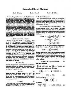
Figure 1.1: Two-dimensional illustration of a separating hyperplane (solid line) and the associated margin-hyperplanes (dashed line). Equations for the hyperplanes are given in 2 canonical form and the margin is then ρ = kwk .

training examples D = {(xi , yi )}i=1...N , where xi ∈ X are the data-points and yi ∈ {−1, +1} are the labels. The result of the training process is a decision function f (x) that is used as a predictor for the labels of new points y ? = sgn(f (x? )). When considering the separable case, it is assumed that the two classes can be separated by a hyperplane (suppose for the moment that X ⊆ Rn ). Given such a hyperplane that separates the positive from the negative examples – a separating hyperplane – let us define the margin ρ as the shortest distance from the hyperplane to the closest data-point. It can be shown that the capacity of the class of separating hyperplanes decreases with increasing margin. Therefore, following Vapnik’s principle, in SVM training the optimal separating hyperplane is computed as the one with the largest margin of separation. In geometrical terms, it is equivalent to the perpendicular bisector of the shortest line connecting the convex hulls of the two classes. In practise it is the result of an optimisation problem that will be sketched briefly in the following. Consider a situation as illustrated in Figure 1.1. Any hyperplane is specified by its normal direction w and its offset b through the equation hw, xi + b = 0. Note that due to the zero on the left hand side, there is a scaling freedom in w and b. Given the direction w of a separating hyperplane and of two parallel margin-hyperplanes going through the closest data-points on each side, a maximal margin is achieved for separating hyperplanes that lie exactly in the middle of the two margin planes. Then w and b can be rescaled such that the margin hyperplanes obey hw, xi + b = ±1.

15

1 Introduction This rescaled representation is called canonical form of a separating hyperplane and eliminates the scaling freedom. The margin of any separating hyperplane in canonical 2 . In order to find the hyperplane form can now be easily computed as ρ = kwk that separates the classes with the maximal possible margin, we solve the following constrained optimisation problem 1 kwk2 2 s.t. yi (hw, xi i + b) ≥ 1, ∀ i = 1 . . . m .

minimise w, b

(1.3)

Here, the margin is maximised while correct classification of the data-points is assured by the constraints (recall that ρ ∼ 1/kwk). As the objective function is quadratic and the constraints are linear, equation (1.3) is a convex optimisation problem. When dealing with the non-separable case, the conditions for correct classification are relaxed to yi (hw, xi i + b) ≥ 1 − ξi to allow some data-points to lie on the wrong side of the separating hyperplane. The amount of misclassification is measured by the slack-variables ξi ≥ 0 ∀i = 1 . . . m that define the distance of a wrongly classified point to its margin hyperplane in canonical units. Naturally, for an optimal solution the amount of misclassification has to be minimised together with the inverse margin. The optimisation problem for the non-separable SVM is thus m

CX 1 ξi minimise kwk2 + w, b 2 m

(1.4)

i=1

s.t. yi (hw, xi i + b) ≥ 1 − ξi and ξi ≥ 0, ∀ i = 1 . . . m . Here the constant C defines the trade-off between separation with a large margin and minimal classification error. The global optimum of the convex problem (1.3) can be found by standard methods of optimisation. Treatment of the non-separable case (1.4) then requires only marginal modifications. First, the constraints are taken into account by introducing Lagrangemultipliers αi ≥ 0 leading to the Lagrangian m

L(w, b, α) =

X 1 kwk2 − αi [ yi (hw, xi i + b) − 1] . 2

(1.5)

i=1

This function is minimised with respect to the primal variables w and b, and maximised with respect to the dual variables α. Stating the conditions for optimality and substituting them back into equation (1.5) leads to the dual optimisation problem (1.6) that is usually solved in practise: maximise α

s.t.

m X i=1

16

m X i=1

αi −

m 1 X αi αj yi yj hxi , xj i 2 i,j=1

αi yi = 0 and αi ≥ 0, ∀i = 1 . . . m .

(1.6)

1.2 Kernel functions When dealing with the non-separable case, the only modification in the dual problem is an upper bound on αi leading to the modified constraints m X

αi yi = 0 and 0 ≤ αi ≤

i=1

C , ∀i = 1 . . . m . m

(1.7)

In practise the dual problem (1.6) is solved by standard methods of convex optimisation, e.g. interior point methods, or by special solvers that are designed for the sparseness properties of SVMs such as sequential minimal optimisation [Platt, 1999]. The resulting decision function is an expansion in the data-points of the form ! X f (x) = sgn αi yi hx, xi i + b . (1.8) i

From the optimality conditions for the Lagrangian (1.5) it can be derived that αi = 0 for all data-points that are correctly classified and lie outside the margin. This confirms the intuition that the optimal separating hyperplane is only determined by the points close to it. The data-samples xi that appear in the expansion (1.8), i.e. that have a αi 6= 0, are called support vectors.

1.2 Kernel functions The linear classification algorithm described above, has been introduced for vectorial data-points xi ∈ X = Rn whose geometrical relations like distances and scalar products have a meaning in the context of the problem to be solved. For several reasons, it turns out to be very useful to map the data into a new feature space, before the classification step. This so-called feature map Φ : x 7→ Φ(x) can be useful to turn a not linearly separable problem into one that can be solved with a linear classifier in feature space. Furthermore, a feature map is the first processing step when the given data is of non-vectorial or even non-numerical nature in order to extract numerical values that describe each data item appropriately. To apply the support vector algorithm to this new data representation, we only have to replace each data-point xi by Φ(xi ) in the formulas for the decision function (1.8) and the dual optimisation problem (1.6) and (1.7) respectively. Interestingly, the data appears only in scalar products that change from hx, x0 i into hΦ(x), Φ(x0 )i. Thus, instead of choosing a feature mapping Φ and then computing the scalar product, it is often computationally more attractive to specify directly the function k(x, x0 ) := hΦ(x), Φ(x0 )i. This function k(x, x0 ) is called kernel function and is positive definite2 if and only if it corresponds to a valid scalar product in some feature space. Therefore, choosing an appropriate positive definite kernel function 2

k(x, x0 ) is a positive definite function if and only if the matrix Ki,j = k(xi , xj ) is a positive definite matrix for all choices of vectors xi . A real valued matrix K is positive definite if and only if it is symmetric and ∀ v : v> Kv ≥ 0.

17

1 Introduction amounts to implicitly working with a (possibly non-linear) data embedding but circumventing at the same time the burden of computing the explicit mapping Φ(x). Note that this so called kernel trick not only enables the geometrically motivated linear support vector algorithm to achieve non-linear decision boundaries in vectorial input spaces but also allows the application to non-vectorial or non-numerical input data. This embedding property will be of great use for later applications where the data-objects are sequences of neural activity and images represented as sets of local descriptors. A more intuitive interpretation of the kernel function is to look at it as a similarity measure for the specific type of data at hand. The dual optimisation problem for an SVM with a given kernel function that is mostly solved in practise is: maximise α

s.t.

m X i=1

m X i=1

m 1 X αi αj yi yj k(xi , xj ) αi − 2 i,j=1

(1.9)

C αi yi = 0 and 0 ≤ αi ≤ , ∀i = 1 . . . m . m

The SVM is not the only algorithm that benefits from the kernel trick. In fact, a number of methods, that can be expressed in terms of scalar products of the data, have been extended with kernels to yield new powerful applications. Among the most prominent are kernel principal component analysis (kPCA, [Schölkopf and Smola, 2002, Chapter 14]), kernel canonical correlation analysis (kCCA, [Kuss and Graepel, 2003]), kernel Fisher discriminant (KFD, [Schölkopf and Smola, 2002, Chapter 15]) to name a few. All these methods are relatively loosely subsumed under the term kernel methods. Inspired by the success of SVMs and other kernel methods the development of kernel functions for specific data types and particular applications has experienced a boost of activity. Standard kernel functions on vector spaces are the linear kernel klinear (x, x0 ) = hx, x0 i, the polynomial kernel kpoly (x, x0 ) = (1 + hx, x0 i)p and the Gaussian radial basis function (RBF) kernel krbf (x, x0 ) = exp(−kx − x0 k2 /2σ 2 ). More advanced kernels have been developed to operate on complex structures like e.g. the string kernel of Lodhi et al. [2002] that will be used in a modified form in Part I, kernels on graphs [Kashima et al., 2003] or kernels on generative models [Jaakkola and Haussler, 1999]. Kernels on sets [Kondor and Jebara, 2003, Wolf and Shashua, 2003] will be applied to images in Part II of this thesis. Endowed with such flexibility, support vector machines have been successfully applied in many fields (see e.g. the web-page of Guyon). In the field of computer vision, applications to handwritten digit recognition [LeCun, 2000] and face detection [Kienzle et al., 2004] represent state of the art algorithms.

18

Part I

Kernel Methods for the Analysis of Neural Activity

The goal of neural science is to understand the functioning of the brain and the nervous system in humans and animals – how an organism can perceive and act, or even think and remember. Scientists collect data about the anatomical structure of nerve cells and nerve fibres and the physiological processes therein. They record electrical traces of signals that are transmitted from the sensory neurons to the cortex and others that evoke activity of the organism’s muscles. Trying to understand the meaning of this electrical activity has lead to many questions: What information do these signals represent? How is this information encoded in the electrical activity – what is the code that is used for communication between distant parts of the nervous system? How does the brain processes all that input when solving certain tasks and how are particular strategies actually implemented by the biological building blocks that we know? Some of these questions can be addressed by a reconstruction analysis. Reconstruction is trying to decode the neural signals. For example when examining the electrical activity of sensory neurons, the goal is to reconstruct the associated variable that describes the corresponding sensory modality. Equivalently, for recordings from the motor pathway, a reconstruction analysis seeks to infer the intended action from a neural signal. Application of different decoding methods and the interpretation of their reconstruction precision can shed light on some of the aforementioned questions. A particular hypothesis about the neural code that is represented by a decoding method can be tested against other hypotheses, assuming that higher reconstruction accuracy correlates with the validity of the implied code. The highest achievable precision can then be used to derive a lower bound on the amount of information that is conveyed by the neural signals under consideration. In response to medical needs and backed by the increasing amount of knowledge and technical expertise that has already been accumulated in neuroscience over the past decades there is a growing interest in development of devices that can directly interact with the nervous system. The engineer’s dream is to build technical systems that can replace missing or malfunctioning parts of the human body (prostheses, artificial sensors for hearing and vision) or to extend it beyond its natural capabilities (thought controlled human-machine interaction). Possible applications include brain-computer interfaces that can help severely handicapped people to interact with their environment, motor-prosthetic devices as a convenient replacement for passive prostheses or more powerful sensory enhancements like hearing aids or even artificial eyes. The challenge is the interpretation of neural signals for the control of external devices or the generation of neural activity patterns as a meaningful input to the brain. The use of neural activity for control involves a reconstruction problem. When building for example a motor-prosthetic device, the prosthesis’ control unit has to decode neural signals measured in the patient’s motor pathway in real time and react upon it with high precision (see for example Wessberg et al. [2000]). Therefore, from an engineering point of view, reliability, speed and precision of the reconstruction step are central questions that crucially determine the overall performance. As a consequence we consider two largely entangled, although different motivations

21

for reconstruction – gaining scientific insight and engineering technical applications. These two viewpoints can sometimes lead to diverging strategies and conclusions when designing and analysing reconstruction experiments. We will refer to this dichotomy frequently throughout Part I and point out which implications follow from the respective viewpoints. Kernel algorithms like support vector machines and Gaussian processes are only recently becoming an accepted tool as reconstruction methods [Shpigelman et al., 2003, Eichhorn et al., 2004, Hung et al., 2005]. Instead, widely used standard methods are Bayesian reconstruction [e.g. Dayan and Abbott, 2001], basis functions [Zhang et al., 1998] or the older population vector method [Georgopoulos et al., 1986]. We believe that kernel algorithms have some advantages in comparison to the classical reconstruction methods that let them appear as an interesting alternative: 1. Non-Euclidean Geometry: By construction, kernel methods easily allow the use of non-euclidean scalar products or distances in input space. Kernel functions can be designed to reflect the notions of similarity that correspond to a particular hypothesis of neural coding. Competing hypotheses are represented by different kernel functions and can be tested within identical algorithms to assess their performance. From a scientific point of view, this is the most interesting feature of kernel methods. 2. Decoding Accuracy: Support vector classifiers have shown competitive or superior performance in a wide range of applications when compared to other machine learning algorithms (e.g. k-nearest neighbour or naive maximum likelihood estimators). We will show in the experimental section that SVMs and Gaussian processes can outperform classical methods for reconstruction in terms of accuracy. As the precision of decoding is one of the key interests when engineering artificial neural interfaces, this feature of kernel methods is important from an application point of view. The application of kernel algorithms to stimulus reconstruction from neural activity patterns will be explored in Part I of this thesis, which is structured as follows. Chapter 2 gives a general introduction to basic concepts of neuroscience where the reconstruction problem is described in detail and classical approaches to this problem are explained. In Chapter 3, this task is reviewed from a machine learning perspective and arguments for the usefulness of kernel machines in this framework are discussed. Moreover, three kernel functions are presented that seem well suited for an application to time series of neural activity, and the underlying assumptions about the neural code are described. The validity of those assumptions is tested in Chapter 4 in a binary discrimination task on data from a generative model that allows to control spike correlations. Furthermore, the kernels are tested in a similar setting on data from neurophysiological recordings at high temporal resolution. A more applied viewpoint is taken in Chapter 5 where the same kernel functions are applied to the extended task of reconstructing eight stimulus conditions from the activity of a population of twenty

22

neurons. In this second set of experiments the impact of algorithmic improvements that were introduced to increase reconstruction accuracy by the use of output space structure is analysed. Finally, an overall discussion of the findings and directions for further research are presented in Chapter 6.

23

2 Fundamental concepts in neuroscience The brain and the nervous system have been subject of research for centuries, but still its structure and functioning remain a largely unresolved secret that is of central relevance for human identity. Insights into the mechanisms and principles that govern our perception and thinking, our reasoning and our decisions would have wide-ranging implications not only in neurobiology and medicine. A clear understanding of the human brain may alter drastically the way we think about ourselves as human beings, about the nature of concepts as the free will, consciousness, responsibility, guilt and conscience. The brain is still one of the few pieces of terra incognita in today’s post-modern world of omnipresent scientific explanations. In the early days of brain research, due to the lack of appropriate measurement devices, phenomenological studies were the only means of inference about the brain – a still relevant example is the classic of von Helmholtz [1870]. Since then, modern science has accumulated huge amounts of data about the anatomical structure of nerve cells and fibres, starting e.g. with Golgi [1903] and Ramón y Cajal [1894–1904], and about the electrical activity of neurons – a field of research that was pioneered by Adrian [1928, 1932]. Studies have been conducted in almost any part of the nervous system and over a wide range of species including the human himself (see e.g. Engel et al. [2005] for a recent review on invasive recordings from human brain). Below, we present a brief summary of facts about the nervous system that are currently common knowledge in neuroscience. General references are the books of Nicholls et al. [1992] and Kandel et al. [2000], a lot of histological details can be found in Braitenberg and Sch¨ uz [1998].

2.1 Brief overview of the nervous system We here summarise a few basic facts about the nervous system of higher vertebrates, in particular humans. This presentation is meant to provide the terminology for the remaining chapters and does not aim at completeness in any respect.

2.1.1 Neurons The human brain contains of the order of 1010 neurons [Braitenberg and Sch¨ uz, 1998, Chapter 4]. Neurons are a major class of cells in the nervous system that can process and transmit information in the form of electrical impulses. Many neurons are highly specialised, and they differ widely in appearance (cf. Figure 2.2). A schematic sketch is shown in Figure 2.1.

25

2 Fundamental concepts in neuroscience

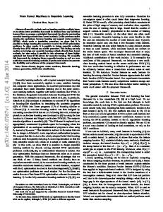
Figure 2.1: Schematic picture of a neuron. The cellular extensions of a neuron are called axons and dendrites and they transmit electrical impulses between neurons and from neurons to other cells of the nervous system. A neuron usually receives electrical impulses through its dendrites and it transmits them to other cells via its axon. Axons end in a special junction called synapse and are often covered with a myelin sheath.

26

2.1 Brief overview of the nervous system

Figure 2.2: Drawing of different neurons stained with the Golgi method. Shape and extension of axons and dendritic tree show a considerable variation across species. (From Rosenzweig et al. [1998].)

27

2 Fundamental concepts in neuroscience Typically, neurons have two types of cellular extensions that connect them with other neurons and conduct electrical impulses along their excitable cell membrane. Dendrites form a profusely branched tree of cellular extensions and are assumed to receive signals from other cells. The axon of a neuron can be much longer than the dendrites (up to 1000 times the diameter of the cell body), and it transmits electrical impulses to other neurons or non-neural cells such as muscles or glands. Most types of axons are covered by an electrically insulating myelin sheath, that increases the speed of propagation of electrical impulses along the axon. Between neurons, signals are transmitted through specialised junctions called synapses. Here the cell membranes of the two neurons almost touch each other and form a gap – the synaptic cleft which is about 20 nm wide. Synapses are asymmetric both in structure and in how they operate. Only the so-called pre-synaptic neuron secretes neurotransmitters, which bind to receptors facing into the synapse from the post-synaptic cell. The pre-synaptic nerve terminal generally buds from the tip of an axon, while the post-synaptic target surface typically appears on a dendrite or a cell body. A pre-synaptic excitation induces an increase in the potential of the post-synaptic neuron in the case of an excitatory synapse or it reduces the postsynaptic potential when transmitted over an inhibitory synapse. Chemical synapses allow the neurons of the central nervous system to form interconnected neural circuits. On average, a neuron in human brain has between 105 and 106 synapses that uz [1998], connect it with up to five thousand other neurons (cf. Braitenberg and Sch¨ Chapters 34 and 35).

2.1.2 Neural activity Axons and dendrites transmit electrical signals that form the basis of communication in the nervous system. These signals consist of potential changes produced by electrical currents flowing across the cell membranes. Currents are carried by ions such as sodium, potassium, and chloride. Neurons use two types of signals: localised potentials and action potentials. The localised, graded potentials can spread only short distances which are usually limited to 1 or 2 millimetres. They play an essential role at special regions, such as sensory nerve endings (where they are called receptor potentials) or at junctions between cells (where they are called synaptic potentials). Localised potentials enable individual cells to perform their integrative functions and to initiate action potentials. The action potentials are regenerative pulses that are conducted rapidly over long distances in the nervous system without attenuation. Neural activity data is acquired by measuring the voltage (in orders of mV) at the tip of a micro-electrode against body liquid in the surrounding region (cf. Figure 2.3). The micro-electrode is placed inside the cell body of a neuron (intra-cellular recording) or close to it (extra-cellular recording). When recording extra-cellular neural activity in regions of high nerve cell density, typically the electrode picks up impulses from more than one neuron in the vicinity of its tip. The goal of spike sorting is to identify action potentials originating from different neurons and to correctly assign

28

2.1 Brief overview of the nervous system

Figure 2.3: Left: Schematic picture of extracellular recording with a microelectrode. The electric potential in the vicinity of one or several neurons is measured against the surrounding body liquid. Right: Sketch of the tip of a so-called tetrode, a special type of micro-electrode that allows simultaneous recording at four spatially proximate points with distances of circa 10 − 40 µm (indicated by the grey areas).

them to their corresponding sources. An experimental improvement that facilitates this task considerably is the use of tetrodes for recording. A tetrode is four microelectrodes in one, i.e. it can record the voltage at four spatially separated points on its tip that have fixed distances of 10 − 40 µm (cf. Figure 2.3, at the right). When recording with tetrodes, slight differences in amplitude and shape of the waveforms in the four channels allow a more robust assignment of spike events to distinguishable sources. Using this and other techniques, modern neurophysiology allows simultaneous recordings from more than hundred neurons at a time (an example is the work of Gray et al. [1995], it also contains additional details on tetrodes and spike sorting). Time series of electrical activity of a single neuron contain variations at several characteristic frequencies. After filtering the signal through a high-pass filter, a sequence of stereotypical waveforms is obtained that have a width of about one millisecond (cf. Figure 2.4). These are the action potentials or spikes, and their shape and duration are virtually identical within an organism and across species. Due to their stereotypical nature, it is commonly believed that most of the information in spiking activity is contained in the times of occurrence of action potentials and not in the exact shape of the individual waveform. Therefore a time series of voltage recordings

29

2 Fundamental concepts in neuroscience A sequence of action potentials 400

Voltage (in mV)

300 200 100 0 −100 −200 −300

0

5

10

15

20

25

Time (in ms)

Figure 2.4: Example of extracellular recordings. The upper panel shows an idealised plot of a sequence of action potentials. Straight lines between waveforms indicate that variations at low frequencies and below a certain threshold are ignored. At the level of abstraction assumed for further analysis, each action potential is considered as a binary event (as indicated in the lower panel). The data was recorded in one channel of a tetrode in primary visual cortex (V1) of a behaving macaque (see Section 2.2.1).

can be abstracted as a sequence of binary events. The electrophysiological process in a nerve cell that produces action potentials requires for every neuron a short period of regeneration immediately after the emission of a spike, during which it is much harder to evoke another action potential. This resting time is called refractory period and is of order of 1 − 2 ms. As a consequence, the time between consecutive spikes in single-cell recordings is never much shorter than the refractory period. In our work we will consider only the high-frequency action potentials for further analysis, although there are indications that slower varying components, so-called local field potentials, can also contain information (see e.g. Bullock [1997], Heeger and Ress [2002, p. 146] or Logothetis and Wandell [2004, p. 744]).

2.2 From stimulus to neural response – principles of encoding In this section we present widely accepted knowledge about neural coding. For more details see e.g. the books of Rieke et al. [1997], Dayan and Abbott [2001] or Gerstner and Kistler [2002]. Two major tasks of the nervous system are the collection and processing of sensory information and the control of the muscular system via motor commands. According to these functions, nerve cells and fibres are structured in a so-called sensory pathway and in a motor pathway. Information about external stimuli is processed and transmitted by neurons along the sensory pathway, starting with sensory neurons (e.g. in the skin or in the retina) and continuing in lower and higher areas of the cortex.

30

2.2 From stimulus to neural response – principles of encoding

Figure 2.5: Schematic view of the visual pathway. Nerve fibres from both eyes cross at the optic chiasm and are re-grouped according to whether they transmit signals from the left or the right part of the visual field. (After Goldstein [1996].)

Neurons and nerves of the sensory pathway can be further subdivided with respect to the sensory modality they are associated with. The connection patterns that were found in the nervous system allow a clear distinction into visual pathway, auditory pathway, olfactory pathway etc. Each of these sensory pathways consists of several stations of processing. Also later stations of the pathway in the cortex – the so-called lower and higher areas – are spatially separated regions, that can be assigned to the type of sensory input they receive, i.e. there is a visual cortex, an auditory cortex etc. Let us consider the visual pathway in more detail (see Figure 2.5). The photoreceptor cells of the retina transform light into neural signals that undergo further processing by other neurons of the retina. These signals are sent to the lateral geniculate nucleus (LGN), that is the next major processor of visual information. The LGN sends projections directly to the primary visual cortex (V1) and in addition receives many strong feedback connections from there. V1 is the earliest cortical visual area. It is highly specialised for processing information about static and moving objects and seems to play a major role in pattern recognition. Neurons in the visual cortex fire action potentials when visual stimuli appear within their receptive field. A receptive field is a small region within the entire visual field. Any given neuron only responds to a subset of stimuli within its receptive field. This property is called tuning. In a series of classic experiments, Hubel and Wiesel [1968] could classify nerve cells in V1 into simple cells and complex cells, according to the types of stimuli these cells respond to. Both types of cells require a specific field-axis

31

2 Fundamental concepts in neuroscience orientation of a dark-light boundary and do not respond to diffuse illumination of the entire receptive field. In contrast to simple cells, the demand for precise positioning of the stimulus inside the receptive field is relaxed in complex cells. The meaning of the signals arising from complex cells, therefore, differs significantly from that of simple cells. The simple cell localises an oriented bar of light to a particular position within the receptive field, while the complex cell signals the abstract concept of orientation without strict reference to position. Although the activity in higher areas in visual cortex can be related to more complex types of stimuli, processing at this stage is in general not yet well understood.

2.2.1 A neurophysiological experiment When setting up an experiment, neurophysiologists try to control the attributes of a stimulus that are correlated with the activity of neurons under investigation; or vice versa, they try to find neurons whose variability in activity correlates with the variability in the presented stimuli. Consider visual stimuli and let s(t) describe the time-dependent stimulus attribute that is relevant for a recorded neuron, i.e. that correlates with its activity. For example, for complex cells in V1, one relevant stimulus attribute is the orientation of a dark-light boundary in their receptive field. Neurons in other areas might respond to more complex stimuli, hence their activity depends on more complex attributes. An example are H1-neurons in fly whose activity is related to the velocity of vertical bars moving across their receptive field, or other neurons in higher visual areas of monkey that are tuned to a predominant direction of movement of random dots. Note that there is a difference between stimuli where the attribute s(t) varies during presentation and stimuli with constant attributes, and that this difference does not necessarily coincide with the division into static and dynamic stimuli. A dynamic stimulus can still appear as a constant attribute to the corresponding neuron whose activity is recorded, e.g. moving vertical bars with a constant velocity appear as a constant stimulus to a fly’s H1-neuron. Thus, this distinction of stimuli depends on the type of neurons under consideration. During a neurophysiological experiment, stimulus attributes are varied – continuously over time or from trial to trial for stimuli with constant attributes – and the activity of neurons is recorded as a time-series a(t). As an example we describe an experiment that was conducted in the neurophysiology department of the Max Planck Institute for Biological Cybernetics, T¨ ubingen by Andreas Tolias and coworkers (Dept. Logothetis). The recorded data-set of spiking activity stems from a population of twenty simultaneously recorded complex cells in primary visual cortex (V1) of a behaving macaque (Macaca Mulatta). It will be analysed in more detail in Chapters 4 and 5. All experiments were conducted in full compliance with the guidelines of the European Community (EUVD/86/609/EEC) for the care and use of laboratory animals and were approved by the local authorities (Regierungspr¨ asidium). The animal’s task was to fixate a small square spot on the monitor while gratings

32

2.2 From stimulus to neural response – principles of encoding

Angle = 0.0

o

Angle = 90.0 o

Angle = 22.5

o

Angle = 45.0

o

Angle = 67.5

o

Angle = 112.5 o Angle = 135.0 o Angle = 157.5 o

Figure 2.6: Sine wave gratings in eight different orientations that were presented as visual stimuli in the neurophysiological experiment described in the text. The contrast level of the patterns is at 30% (named ’high contrast’ in the text).

of eight different orientations (0 o , 22 o , 45 o , 67 o , 90 o , 112 o , 135 o , 158 o ) and two contrasts (2 % and 30 %) were presented (see Figure 2.6). The stimuli were positioned on the screen so as to cover the classical receptive fields of the neurons. A single stimulus of fixed orientation and contrast was presented for a period of 500 ms, i.e. during the epoch of a single behavioural trial. All eight stimuli appeared 30 times each and in random order, resulting in 240 observed trials for each contrast condition. Recordings were performed extra-cellularly using tetrodes inserted in the specified region of the animal’s cortex. Spike waveforms were sampled at 32 kHz, then highpass filtered, thresholded and time-stamped. Signals from different neurons recorded by the same tetrode are separated afterwards during spike-sorting. Figure 2.7 shows a subset of the resulting spike sequences of a particularly active neuron, called neuron no. 7. In the upper panel, 30 trials of 800 ms of recorded activity are shown for two stimulus conditions; in the lower panel, the 500 ms time window of stimulus presentation is indicated. When comparing the neural responses of neuron 7 for the two stimulus conditions, one can observe two features that are characteristic for neural coding. First, the difference between the two conditions in the number of spikes in a sequence during stimulus presentation is larger than the variance of this quantity over spike sequences of a fixed condition. Second, in the time window between 250 ms and 400 ms the temporal distribution of spikes exhibits a typical pattern that is different for the two stimulus conditions and repeatedly appears in almost all trials. The observations of such features lead to the formulation of two principles of neural coding, namely rate coding and temporal or correlation coding. In rate coding, spikes are assumed to be independent and only their frequency is related to the stimulus attributes. In

33

2 Fundamental concepts in neuroscience

157.5o and 135o

Activity of Neuron 7 10 20 30 10 20

Stimulus

30

0

100

200

300

400

500

600

700

800

Time in ms

Figure 2.7: Neural activity of a complex cell in macaque primary visual cortex. For two orientation angles of a visual stimulus, recorded spike sequences of 800 ms from 30 trials are shown (see text for details). The bottom panel indicates stimulus on- and offset. Comparing the differences of spike sequences between the two stimulus conditions illustrates the concepts of rate coding and temporal coding.

contrast, in temporal and correlation codes the timing of spikes, relative to stimulus timing (e.g. stimulus onset) or relative to other spikes, conveys information. Before these concepts are explained in more detail in the next sections, we need to define some notation and briefly comment on the way neural data is represented numerically.

2.2.2 Data representation of neural activity Single neuron data Let a(t) be the analog voltage signal representing the activity of a single neuron over time. Through filtering and thresholding spike events are extracted from this signal and can be represented as a set t := {ti } of times ti at which a spike occurred. The cardinality of that set |t| is the total number of spikes in the sequence. The set t contains all the information we consider for further analysis. In practise however, we will not work with this representation of spike events as absolute times, but prefer a row vector v = (v1 , v2 , . . . , vNb ) of Nb bins of spike counts, binned at different temporal resolutions. Each component vj indicates the number of spikes in an interval [(j − 1) ∆t, j ∆t[ of length ∆t. The temporal resolution or bin-width ∆t of this representation determines at what precision the temporal position of spikes can be resolved. Under the assumption that no neural code requires a temporal precision higher than the width of a spike waveform (1 ms), a bin-size of ∆t = 1 ms is the highest meaningful resolution and smaller bin-sizes do not add information. To get a representation that is comparable for different bin-widths, firing rates are used instead of spike counts. The firing rate rj in an interval [(j − 1) ∆t, j ∆t[ is the spike count divided by the interval length: rj = vj / ∆t. We will refer to

34

2.2 From stimulus to neural response – principles of encoding the mean firing rate or average firing rate of a sequence t as the totalPnumber of b spikes in this sequence divided by the recording time T : r = |t| / T = N j=1 vj / T . Thus, a sequence of spikes can be equally represented as vector of spike counts v = (v1 , v2 , . . . , vNb ) or a vector of firing rates r = (r1 , r2 , . . . , rNb ), or it is summarised by a single number r. Data from multiple trials will be indexed with an upper index i = 1 . . . Ntr as v(i) , r(i) or r(i) . Multiple neurons When analysing a population of neurons, often their neural activity in a certain time interval is considered, and called activation state of that population. We denote the activation state of Nn neurons as a column vector of spike-counts vj = (vj1 , vj2 , . . . , vjNn )> . Thus, a sequence of Nb activation states of Nn neurons is denoted as a matrix  1 1  v1 . . . vN b 2   v12 . . . vN  b  (2.1) v =  .. ..  .  . .  Nn v1Nn . . . vN b

Identical notation applies to firing rates r, and multiple trials are again indexed with neuron, (trial) an upper index (i) which leads to the notation scheme: vbin . If necessary, the meaning of bold symbols will be specified explicitly to avoid ambiguities. When analysing recordings of a neurophysiological experiment, often the stimulusresponse pairs of each trial are summarised in a data-set D = (v(i) , s(i) ) or D = (i) (i) (r , s ) where s(i) denotes the stimulus attributes.

2.2.3 Rate coding From neurophysiological experiments we know the stimulus attributes that induce activity of a particular neuron. In rate coding, the relation between stimulus and activity of a neuron is quantified more precisely in mathematical terms with the notion of a tuning function. 2.2.3.1 Tuning function of a single neuron Adrian [1928] was the first scientist who measured action potentials of single cells and he extensively studied the relation between attributes of a stimulus and the induced neural activity in early sensory pathway. He established the concept of a rate code, i.e. that the number of spikes per unit time – the firing rate – encodes the stimulus attribute. For example, he found that for haptic stimuli the stimulus intensity, the pressure applied, is proportional to the firing rate of the stimulated sensory neurons. Encoding of stimulus attributes by firing rate can be found in many parts of the nervous system and also applies to complex cells in primary visual cortex. Figure 2.8 shows mean firing rates of complex cell no. 7 that was recorded in the neurophysiological experiment described in Section 2.2.1 above (see also Figure 2.7).

35

2 Fundamental concepts in neuroscience Tuning function of a complex cell in macaque V1 Average firing rate in Hz

60 50 40 30 20 10 0

0

22.5

45

67.5 90 112.5 Stimulus angle in degree

135

157.5

180

Figure 2.8: Tuning function of complex cell no. 7 (see text for details). Crosses indicate mean firing rates for all eight stimulus conditions averaged over trials. The solid line is a cosine tuning function of the form (2.3) fitted to the data.

The plot shows the cell’s mean firing rate averaged over 30 trials for all eight stimulus conditions. Typically, complex cells are tuned to a specific orientation, i.e. they are maximally active when dark-light boundaries with this orientation appear in their receptive field. As one can approximately infer from Figure 2.8, neuron no. 7 is tuned to an orientation somewhere between 100 o and 145 o . The exact relation between a stimulus attribute s and a neurons firing rate is described by the tuning function λ(s). This function is determined from the recorded data for each neuron individually, and it contains all information of a rate code. In most cases a tuning function λ(s) is either represented as an analytic function λθ (s) depending on parameters θ or as a vector of numeric values in a discretized stimulus space. We call the first type a parametric tuning function. The values of its parameters are estimated by a least squared (i) error fit of the parametric family λθ to (i) the data-set of recorded activity D = (r , s ) θ? = argmin θ

Ntr 2 X λθ (s(i) ) − r(i) .

(2.2)

i=1

For orientation sensitive complex cells like neuron no. 7, a cosine function of the form s − θ2 (2.3) λθ (s) = θ0 + θ1 cos θ3 is most commonly assumed. The second type of representation is called empirical tuning function and is often used in a discrimination setting where the set of possible stimulus attribute values is discrete: s ∈ {S1 , S2 , . . . , SNC }. Each component λ(Sk ) of an empirical tuning function is simply the mean firing rate averaged over all trials

36

2.2 From stimulus to neural response – principles of encoding with a fixed stimulus condition Sk λ(Sk ) =

1 N (Sk )

X

r(i) .

(2.4)

i : s(i) =Sk

In both cases, we will refer to values of a tuning function as λ(s), may it be a numerical entry of an empirical tuning function or the evaluation of a parametric tuning function. In the example in Figure 2.8, the crosses represent an eight-dimensional empirical tuning function and the solid line is a parametric tuning function of the form (2.3). 2.2.3.2 Population coding Although some types of stimuli can be reconstructed fairly precisely from the activity of a single nerve cell, the nervous system of most highly developed organisms uses large numbers of neurons to represent information. This operating principle is named population coding and entails several advantages, including a reduction of uncertainty due to neural variability and the ability to represent stimulus attributes over a wider range with high precision. Individual neurons in a population typically have different but overlapping selectivities and sensitivities, so that many neurons respond to a given stimulus at the same time. More details about population coding can be found in the book of Dayan and Abbott [2001, Chapter 4] or in a recent review by [Averbeck et al., 2006].

2.2.4 Beyond rate coding – temporal codes and correlation codes Since the pioneering work of Adrian [1928, 1932] the concept of rate coding has been widely adopted and many experimental results were interpreted under the assumption that information is encoded exclusively in the mean firing rate of a spike sequence. However, experimental results also indicate the relevance of other coding principles in certain parts of the nervous system. In particular in the last fifteen years, neuroscientists have concentrated much more on the role of individual spikes and spike times, inter-spike intervals and correlations of spikes in a sequence, or correlations among a population of neurons. Because timing of individual spikes plays an important role in these types of coding, they are called temporal codes. Other codes that depend on coincident spike events or more generally on the relative temporal positions of spikes are named correlation codes. Whether temporal or correlation coding plays an important role in human or animal brain is the topic of a still ongoing and very active debate. Without taking a serious standpoint nor aiming at completeness, we would like to point out a few facts that support the existence of such codes: 1. Temporal structure in neural activity is visible. In many parts of the nervous system scientists have recorded spike patterns of high regularity and reproducibility. Often, a correlation between pattern and stimulus condition could

37

2 Fundamental concepts in neuroscience be established. One of many examples are recordings in the olfactory system of locust that was extensively studied by Laurent [2002]. Temporal structure is also apparent in the data-set shown in Figure 2.7. Clearly in the time window between 250 ms and 400 ms there is a structure in spike times that is stable over trials in one class and varies with the stimulus condition. 2. Reaction times have been measured in psychophysical experiments for different types of tasks. They indicate that based on the physiological limits of nerve cells, only very few spikes (one or two) could have been transmitted from one layer to the next along the sensory and motor pathway to eventually evoke the desired action [Thorpe et al., 1996] (see also e.g. VanRullen et al. [2005], Johansson and Birznieks [2004]). To estimate a firing rate, at least two spikes are needed, and reliable estimates require averaging over a substantial time window or a population of many neurons. Such short reaction times do not allow for precise estimation of firing rates – but still behavioural studies show that humans can reproducibly perform precise actions very quickly. This is a strong indication, that information about sensory input cannot only be encoded in firing rates of single neurons alone. 3. Discrimination experiments on spike-data recorded in fly’s H1-neuron show that the discriminability of two conditions increases significantly when a distribution of temporal spike patterns is taken into account, compared to the discriminability that can be achieved from spike count distributions alone (see Rieke et al. [1997, Figure 4.22]).

2.3 Reconstruction – decoding of neural activity 2.3.1 Motivation In the previous sections we exemplified on the visual system how neurons in sensory pathway respond to particular stimuli. Their responses, the neural signals, are symbols that do not resemble in any way the external world they represent. When we see, not the pattern of light intensity that falls on our retina is transmitted, but millions of spike sequences reach the brain through our optic nerve. When we hear, not the acoustic waveforms are processed by the brain, but patterns of spikes from roughly thirty thousand auditory nerve fibres. All the myriad tasks our brains perform in the processing of incoming sensory signals are based on these sequences of spikes. In order to act on the results of these computations, the brain sends out sequences of spikes to the motor neurons. Spike sequences are the language in which the brain receives sensory input, the language the brain uses for its internal operations, and the language of the commands that are sent out to the organism. An essential task of computational neuroscience is to understand this language, to decode the significance of spike sequences, and after all to test if this linguistic analogy is at all helpful.

38

2.3 Reconstruction – decoding of neural activity

Amplifier Filter

Spiketrains

Stimulus recording of neuronal activity

Strue

Srec

Reconstruction

Figure 2.9: Schematic diagram of a reconstruction analysis for the example of complex cells in primary visual cortex. The stimulus angle is reconstructed from the preprocessed neural activity of each trial and compared to the true attributes of the stimulus shown.

What does it mean to understand the neural code? Historically one fallacy was the idea of a little homunculus sitting inside the head. He takes the perspective of the brain and tries to solve the tasks that usually the brain is confronted with. The little man observes a continuous influx of myriads of spike trains that are collected by the sensory neurons. From this he forms the percepts of the world and finally acts upon it. Although this viewpoint is problematic in the sense that thereby one can never get to the true essence of what it means to perceive and experience the world, it still provides a useful concept when analysing neural activity. We as observers are inevitably in the situation of a homunculus when we measure neural activity at some point of the nervous system and try to understand what these signals could mean to the organism. In this sense understanding the neural code means to be able to act as an imagined homunculus. A reconstruction analysis is one step in the technical realisation of this programme. The aim of reconstruction is to infer the stimulus attributes from the neural response that was recorded at some point in the sensory pathway. Although in the thesis at hand only reconstruction in sensory pathway is considered, the same analysis can be applied to neurons of the motor pathway, where attributes of motor actions are the target values for reconstruction. For the example of static visual stimuli the reconstruction process is illustrated schematically in Figure 2.9. In a neurophysiological experiment, visual stimuli with varying attributes are presented to an organism in a set of trials, and neural activity of the responding nerve cells is recorded. After preprocessing, a reconstruction method is used to infer the stimulus attributes in each trial srec from the recorded spike sequences. When comparing srec with the true value strue , which is known from the experimental conditions, the difference between the two provides an estimate for the quality of the applied reconstruction method. Two kinds of conclusions can be drawn from such a setup. First, under the as-

39

2 Fundamental concepts in neuroscience sumption that methods based on valid hypotheses about neural coding achieve higher accuracy than other methods that do not capture essential features of the code, reconstruction allows testing of neural coding paradigms. The quality of a particular method directly relates to the hypotheses it implements, and wrong hypotheses should on average achieve worse results. Second, the highest achievable reconstruction accuracy indirectly provides a lower bound on the amount of information about the stimulus that is conveyed by a spike sequence. If a method can perfectly reconstruct the stimulus from neural signals, it implies that all information about the reconstructed attributes must be contained in the data at hand. However, only a lower bound on this information is obtainable since any reconstruction method might be suboptimal.

2.3.2 Methods As implicitly mentioned above, the choice of a reconstruction method depends on the assumptions about neural coding that one is willing to make. We give a brief overview of classical approaches to reconstruction that, like most of the standard methods, rely exclusively on rate coding, i.e. they assume that a neuron’s tuning function contains all relevant information. The two methods for population decoding and the Bayesian reconstruction method will be applied in Chapter 5. 2.3.2.1 Single neurons To reconstruct a stimulus attribute srec from the given firing rate rˆ of a single nerve cell, the most direct approach would be to search for the stimulus value where the tuning function is closest to rˆ srec = argmin |ˆ r − λ(s)|2 .

(2.5)

s

For parametric tuning functions this minimum is found by analytic measures, for empirical tuning functions an exhaustive search over the stimulus space yields the answer. 2.3.2.2 Population decoding When decoding the activity of neuronal populations the question arises how to optimally combine information that is distributed over many neurons. Although here as well, almost all approaches assume rate coding for the individual neurons, additional difficulties come from possible interactions of neuronal firing and so-called noise correlations (a recent review on these issues was given by Averbeck et al. [2006]). We restrict our presentation to approaches that assume independent neurons and neglect any interactions among multiple neurons. In this case the individual tuning functions can be concatenated to a population tuning function as > λ(s) = λ1 (s), λ2 (s), . . . , λNn (s) . (2.6)

40

2.3 Reconstruction – decoding of neural activity Let D = (r(i) , s(i) ) i=1...Ntr be the data-set of recordings from Ntr trials and Nn neurons. The elements r(i) represent (Nn ×1)-matrices, i.e. column vectors of average firing rates as introduced with the notation in Section 2.2.2. Vector methods Vector methods were invented to reconstruct directional or positional attributes of a stimulus, e.g. for reconstruction of wind directions from neural activity in the cercal system of cricket [Theunissen and Miller, 1991] or to infer position information from hippocampal place cells in rats [Zhang et al., 1998]. One of the first methods to reconstruct directions from multiple neurons was presented by Georgopoulos et al. [1986] under the name population vector. In the original work the authors could discriminate between eight different movement directions in 3D-space from recordings in primary motor cortex (M1) of a rhesus monkey. The population vector approach assumes that each neuron has a corresponding preferred direction (n)

spref = argmax λn (s)

(2.7)

s

where the tuning function achieves its maximum. Here we used a bold symbol for the stimulus attribute s to emphasise its vectorial nature. The preferred directions of neurons are assumed to be equally distributed among the population. To reconstruct the stimulus vector spop.vect from a given activation state of a population ˆr, each neuron’s preferred direction is weighted by its activity relative to its maximum firing rate rnmax and the vector sum gives the result spop.vect =

N X rˆn (n) spref . max rn

(2.8)

n=1

Note, that when inferring positions rather than directions the length of the vector spref is crucial for reconstruction precision, whereas for inference of directions a neuron’s preferred direction is usually normalised to |spref | = 1. Template matching The idea of template matching is very intuitive. To reconstruct a stimulus attribute stemplate from an activation state vector ˆr, the stimulus that created the best matching activity pattern is selected from the estimated tuning functions stemplate = argmax hˆr, λ(s)i .

(2.9)

s

In machine learning terminology this approach would correspond to a nearest neighbour classifier. It seems to work best in discrimination settings where the set of stimulus attributes s ∈ {S1 , S2 , . . . , SNc } is limited, and reconstruction has to choose one of the Nc possible outcomes.

41

2 Fundamental concepts in neuroscience 2.3.2.3 Bayesian reconstruction When looking at examples of neural recordings (e.g. Figure 2.7) one can generally observe a certain amount of variance among the activity patterns. A part of this variance can be explained by an encoding model relating some properties of spike sequences, as e.g. their mean firing rate, to the variability of stimulus attributes. The remaining variance inside a class of neural responses belonging to identical stimuli that cannot be explained by an encoding model is called noise. The origins of this unexplained variance can be manifold. It could be due to some hidden variables that are not controlled during the experiment, as for example cortical input from other cells to the measured neurons. Noise can also be induced by errors in the elaborate measurement process, e.g. during thresholding or spike sorting, or it could be due to physiological processes in the nerve cell that are of chaotic or truly random nature. In any case, this variability suggests a stochastic description of the encoding process, the translation of stimuli into spike sequences. During reconstruction the inverse problem of decoding spike sequences and inferring the corresponding stimulus attribute has to be solved. In the following we will show how these two questions are related by the rules of probability and give a brief introduction into what is commonly referred to as Bayesian reconstruction. Again, the stimulus attribute is denoted with s and the set of event-times that represent the corresponding spike sequence is abbreviated with t. A stochastic decoding model would be expressed as the conditional probability distribution p(s|t), the probability that stimulus s was shown given that the sequence t was recorded (sometimes also called the response-conditional ensemble [Rieke et al., 1997]). The encoding model is a probabilistic model p(t|s) that specifies the probability of a certain spike sequence t to be generated as response to a stimulus with the attribute s. The decoding model is related with the encoding model via Bayes rule: p(s|t) =

p(t|s) · p(s) . p(t)

(2.10)

In the context of Bayesian inference the probability p(s|t) is named the posterior distribution, p(t|s) is the likelihood, p(s) is the prior distribution over stimulus attributes and p(t) is the evidence or marginal likelihood. To be able to compute the posterior, i.e. to get the decoder and do reconstruction, we have to make assumptions about the encoding process, i.e. we have to specify the likelihood p(t|s) and we have to know the prior distribution over stimuli p(s). In experimental situations with artificial stimuli often the prior p(s) is chosen as the relative frequency of presented stimuli, and the focus of research lies on the encoding model p(t|s).1 Note that it is not nec1

However, a living organism in a real world scenario, where stimuli are not controlled and thus not of highly reduced variability as in the experiments, is not in this comfortable situation. Considering for example the visual system, stimuli are distributed according to natural image statistics, i.e. the characteristics of images that appear regularly in the organism’s habitat. Knowledge about the prior distribution of visual input p(s) can be a crucial part of a fast and accurate vision system and therefore knowledge about natural image statistics is generally of high interest.

42

2.3 Reconstruction – decoding of neural activity essary to specify explicitly the marginal likelihood p(t). It can be determined as the R normalising constant of the nominator of Equation (2.10): p(t) = ds p(t|s) p(s). Suppose we had complete knowledge about the likelihood function p(t|s) and the prior p(s) for a particular organism in a particular experiment. Hence, to infer something about the stimulus from a particular spike-sequence ˆt we compute the posterior p(s|ˆt) that contains everything we can possibly know about the decoding process. A homunculus that was forced to act upon sensory input could use this probability distribution to minimise the risk R(ˆ s, ˆt) of a decision that assumes the spike-generating stimulus attribute to be sˆ based on a given loss-function L(s, s0 ) Z R(ˆ s, ˆt) = ds p(s|ˆt) L(s, sˆ) . (2.11) For example, when assuming the mean squared error as loss-function L(s, s0 ) = |s − s0 |2 , the mean of the distribution s¯ is the optimal point estimate Z Z 2 ds p(s|ˆt) s − s0 . (2.12) s¯ = E [s] = ds p(s|ˆt) s = argmin s0

Another choice of interest is the most probable value for the stimulus attribute, i.e. the value of s where the posterior distribution p(s|ˆt) is maximal. This point estimate is commonly referred to as maximum a posteriori (MAP) estimate. If the prior distribution p(s) in Bayes’ formula (2.10) is non-informative, i.e. it does not depend on the value of s, we can neglect p(s) and the normalising denominator, and the posterior is proportional to the likelihood: p(s|ˆt) ∝ p(ˆt|s). In this case the most probable value is called maximum likelihood (ML) estimate of s. The encoding model All assumptions and knowledge about the structure of the neural code enter through the likelihood function p(t|s). Its functional form and its parameters fully describe the encoding process. To illustrate the machinery of Bayesian reconstruction, we will assume simple rate coding. It relies on the assumption of independent spikes, i.e. the probability of a spike at time t is independent of all other spikes at times other than t and is uniquely determined by a global firing rate λ. A random process with such properties is called Poisson-process. The number of spikes N in a sequence of unit length generated by a Poisson-process is distributed according to a Poisson-distribution with rate λ p(N ) = Poisson (N ; λ) =

λN exp(−λ) . N!

(2.13)

The average mean firing rate of such sequences is λ. For a rate code the relation between the stimulus attribute and the mean firing rate is fully specified by the tuning function λ(s). We will assume a parametric tuning function λ and show θ (s) (i) later how its parameters θ can be inferred from a data-set D = (r , s(i) ) by using Bayes’ formula once more. Our knowledge about the parameters is represented

43

2 Fundamental concepts in neuroscience in a probabilistic manner by the posterior p(θ|D). In a fully Bayesian treatment the likelihood is an integral over all possible parameter values weighted with their respective probability Z dθ p(t|s, θ) p(θ|D) p(t|s) = Z (2.14) = dθ Poisson (|t|; λθ (s)) p(θ|D) . For the sake of simplicity in practical applications the integral in Equation (2.14) is often replaced by a MAP or ML point estimate of the parameter values ˜ p(t|s) = p(t|s, θ)

with θ˜ = θMAP or θ˜ = θML

where θMAP = argmax p(θ|D)

and θML = argmax p(D|θ) .

θ

θ

The posterior distribution of the parameters p(θ|D) is inferred from the data-set by applying Bayes rule again p(D|θ) p(θ) p(θ|D) = p(D) where p(D|θ) is the likelihood function for the whole data-set D given the parameter values θ. Under the reasonable assumption that all trials are independent this expression factorises into a product of Poisson-distributions p(D|θ) =

=

Ntr Y i=1 N tr Y

p(t(i) |θ, s(i) ) (2.15)

Poisson |t(i) |; λθ (s(i) ) .

i=1

Any assumptions about the parameters can be put into the prior distribution over parameters p(θ), for example a sensible range for the inverse frequencies θ3 of the cosine ansatz (2.3).

44

3 Reconstruction with kernel methods The main contribution in Part I of this thesis is the exploration of kernel methods for stimulus reconstruction from neural activity. In this chapter we will explain why reconstruction can be seen as a learning problem and why it is attractive to solve this task with kernel methods. We will introduce three kernel functions that seem particularly well suited for sequences of neural activity patterns and point out the associated hypotheses about the neural codes they are likely to detect.

3.1 Reconstruction as a learning problem In reconstruction of sensory information, one tries to establish a relation between an attribute s of a stimulus and the associated neural activity t that was measured while the stimulus was presented. In almost all methods, some properties of the neural population have to be estimated before the method can be used for reconstruction. For example the neuron’s tuning function or its preferred direction (cf. Section 2.3.2) are estimated from the data by using some of the measured (t(i) , s(i) )-pairs. Furthermore, the reconstruction model is determined by other design decisions, e.g. the choice of a parametric family for the tuning function (like Equation (2.3)) or the choice of the model class itself (e.g. linear models). From a machine learning perspective, all these steps can be identified with concepts of inductive learning. The estimation of neuron properties is the training phase of a learning algorithm. Choosing a model class or a particular type of tuning function restricts the richness of functions that can be implemented by the reconstruction method, and this can be viewed as a regularisation step. Moreover, Bayesian reconstruction (see Section 2.3.2) is in itself a framework for inductive learning and these concepts have their natural correspondence in Bayesian inference (e.g. regularisation is equivalent to specifying a prior distribution over model parameters and performing MAP inference). Therefore, by making the correspondences explicit, we will treat reconstruction as a learning problem and apply the machinery of machine learning. In particular we will maintain a clear separation of training and test data and compute generalisation errors to assay the validity of a reconstruction model. As learning algorithm we apply kernel methods that have some interesting properties which make them appealing for reconstruction. In particular we will use support vector machines for the analysis in Chapter 4 and additionally Gaussian processes and other learning algorithms for the experiments presented in Chapter 5.

45

3 Reconstruction with kernel methods Besides their current popularity in the machine learning community, kernel algorithms are interesting for an application in reconstruction for two reasons. First, they allow by construction a non-linear geometry in input space – a feature that is very likely to be useful when aiming to decode temporal codes and correlation codes in spike sequences (see e.g. the related discussion by Victor [2005a]). Second, a specific coding hypothesis is encapsulated solely in the kernel function. This property facilitates a straightforward comparison of different hypotheses under identical conditions, which is an essential goal of reconstruction. Furthermore, kernel methods (such as SVMs and Gaussian processes) have shown competitive performance in other application domains and exploring their usability could improve decoding devices in biomedical engineering.

3.2 Kernels for patterns of neural activity When using kernel methods, the question arises what kernel functions are suitable for the analysis of spike sequences or sequences of firing rates. This leads to the more profound question, what general properties a similarity measure on spike sequences should have. As mentioned above, most common approaches to reconstruction assume rate coding. However, in this study we are interested in finding structures in the data in addition to rate codes. In the previous chapter we briefly reviewed arguments that support the existence of such structures, but there is an ongoing and active debate about these issues. It is still unclear how much rate codes and temporal or correlation codes contribute to the transmission of information and their importance may vary depending on the part of the nervous system under investigation. The main assumption that most researchers would agree on, is that similar stimuli are encoded by similar spike sequences. Naturally this statement depends critically on the concept of similarity that is assumed. Smoothness and similarity depend on the metric or scalar product of the vector space where spike sequences are embedded into. Concepts of smoothness vary from standard smoothness in Euclidean space to rather complex models that encode smoothness in their parameters (e.g. smoothness induced by the Fisher kernel [Jaakkola et al., 1998], see also [Oliver et al., 2000]). At this point the strength of kernel machines comes into play. The inherent geometry and thereby the notion of smoothness are defined uniquely by the kernel function. Thus, from a kernel viewpoint we have to define what it means when two sequences are similar. This means, we need to specify what kind of variability in a sequence of spikes is attributed as noise and what kinds of variation change the information conveyed by this sequence. Given that the debate about the principles of neural coding has not settled yet, we will state assumptions/hypotheses of what might be relevant properties and then present kernel functions that feature these properties. In the subsequent two chapters, tests of their accuracy in reconstruction are presented that imply indications for the

46

3.3 Spikernels validity of the underlying paradigms. As a baseline, we apply the RBF-kernel kr − qk2 krbf (r, q) = exp − 2σ 2

.

(3.1)

olkopf and Smola [2002], that using the RBF-kernel It has been shown, e.g. see Sch¨ penalises all order derivatives and therefore induces smoothness for a standard Euclidean embedding of two spike sequences r and q. An SVM with this kernel function allows non-linear class boundaries but contains a linear classifier as the limit-case σ → ∞. In the remainder of this chapter we will present three kernel functions that correspond to other notions of similarity which are thought to be relevant for spike sequences. The basic assumption that all three similarity measures rely on is the idea of a correlation code that encodes information through the appearance of typical spike patterns in the data. Each instance of a pattern might be distorted by noise and sensitivity to the temporal position of its occurrence might vary. We will briefly summarise the hypotheses underlying our proposed kernel functions before they are described in detail. The homogeneous spikernel considers weighted contributions of patterns of different lengths up to a maximum number of bins and allows arbitrary temporal positioning of these patterns in the two sequences. Slight distortions of the patterns are tolerated and their contribution to the kernel value is averaged over the whole length of the two sequences. Local alignment kernels are defined by the similarity of the longest pattern matching among the two sequences, also independently of its temporal positioning. In contrast, global alignment tries to match the two sequences over their whole length and assigns the quality of this match as similarity value. Therefore it is more sensitive to patterns at larger scales and their position in the sequence. In the formulation presented below, application of these kernels to spikes sequences or sequences of firing rates is a novel contribution to the field of reconstruction.

3.3 Spikernels In this section we will present a kernel for sequences of firing rates that has been used for SVM based reconstruction of dynamic stimuli. Problems that occur when applying it to static stimuli in a discrimination scenario are discussed, leading to a modified version of this kernel function.

3.3.1 Original spikernel A recent study that used kernel methods for reconstruction was the work of Shpigelman et al. [2003, 2005] who tried to infer hand movement velocities from recordings in macaque primary motor cortex. The authors introduced a new kernel function, the

47

3 Reconstruction with kernel methods so-called spikernel, as a similarity measure for patterns of firing rates recorded from a single or multiple neurons. The design of this kernel is based on four assumptions that are repeated in the following: 1. The first assumption commonly believed by neuroscientists is that firing rate patterns can be considered to be similar if their binned representations differ only slightly in a bin-by-bin comparison, i.e. have a small Euclidean distance. 2. The encoding of external stimuli in the sensory pathway or motor commands in the motor pathway may result in highly specific patterns. Such a pattern of spike counts may change in a highly nonlinear manner as a function of behaviour or of the external stimulus variable [Segev and Rall, 1998]. This assumption is commonly made in models of neural computation [Pouget and Snyder, 2000]. 3. Two firing patterns, although similar, may be misaligned in time. For their similarity to become apparent, e.g. in terms of small Euclidean distance, it might be necessary to realign them by introducing a certain time shift. In comparing patterns, the induced score should be the higher the smaller this time shift is. Biological plausibility for time shifted patterns may stem from the spatial distribution of synaptic inputs on cortical cells’ dendrites [Magee, 2000]. 4. Patterns of spike counts that encode similar values of an external target variable at time t may be similar (in the sense described above) at that time but rather different at times t±δ when the external variable is no longer similar. Therefore similarity of patterns is weighted higher around a time of interest (i.e. the time of prediction) than at points in time that are further apart. Note, that the fourth assumption is specific for reconstruction of dynamically changing target variables. In the original work these were motor commands for hand moving velocities that change continuously. Hand movements with a particular velocity might be preceded or followed by movements with arbitrarily different velocities. Therefore the neural activity at the time of interest is more important than spikes that occurred some time before or after this point. If, in contrast, the kernel should be applied in a discrimination setup with static stimuli, some modifications are necessary that will be discussed in Section 3.3.2. Based on these assumptions, Shpigelman et al. [2003] derive the design of the spikernel by exploiting the analogy between sequences of firing rates and sequences of letters – i.e. text. Inspired by the string kernel [Lodhi et al., 2002] that was successfully applied in text-classification, its feature map is modified for an application to sequences of firing rates. To understand the basic idea of the spikernel it is most insightful to have a look at its feature map rather than at the kernel itself. A sequence of firing rates r of length |r| is mapped to a function Φr (u) on Rn by X n Φ : r 7→ Φr (u) , where Φr (u) = C 2 µd(ri ,u) λ|r|−i1 . (3.2) i∈In,|r|

48

3.3 Spikernels The function Φr (u) specifies the similarity of sequence r to an arbitrary sequence u of length n = |u| ≤ |r|. When thinking of the function Φr (u) as an infinite dimensional vector, u can be thought of indexing the dimensions in the associated feature space. In the formula above, In,|r| is the set of all ordered n-tuples i = (i1 , . . . , in ) of indices i1 < i2 < . . . < in ∈ {1, . . . , |r|} and the sum runs over all such tuples i. Thus, ri is an ordered sub-sequence of r of length n composed of ri = (ri1 , . . . , rin ). C is a normalisation constant and λ, µ ∈ [0, 1] are parameters of the kernel. The µ-part of the sum is an exponential weight depending on the similarity of a sub-sequence ri with the sequence u, that is measured in accordance with assumption one (see P above) by the squared Euclidean distance d(ri , u) = nk=1 krik − uk k22 . The λ-part in Equation (3.2) implements a down-weighting of contributions from sub-sequences that begin far away from the end of sequence r as it is required by the fourth assumption. The application scenario that the authors had in mind when constructing the spikernel was the reconstruction of a continuously varying target variable at time tpred from the preceding time series of neural activity. Therefore the prediction time, i.e. the time of interest, is at the end of the input sequence. Note, that assumption three is only indirectly implemented by the λ-term. In contrast to the string kernel, where the total length of all gaps in a sub-sequences is penalised by a factor ∝ λin −i1 , only the starting index i1 is considered in the feature map (3.2). For the sake of simplicity we introduced the above feature map for sequences of firing rates stemming from single neuron recordings. When extending the kernel to a population of Nn neurons, a single entry rj in the sequence r is an Nn -dimensional column vector containing the firing rates of all simultaneously recorded neurons in one particular time bin (cf. Section 2.2.2). The coordinate u then an Nn × nPbecomes n matrix u ∈ RNn ×n and the Euclidean distance d(ri , u) = kr − uk k22 is a ik k=1 difference of vectors rather than scalars. For a fixed length n of considered sub-sequences, the kernel kn (r, q) of two sequences r and q is computed from the feature map Φr (u) by evaluating the standard scalar product in function space, i.e. via integration over the coordinates u Z kn (r, q) = hΦr (u), Φq (u)i = du Φr (u) Φq (u) . (3.3) RNn ×n

By finding recursive relations for Φr (u) the kernel can be computed in time O(|r| · |q| · n) as a dynamic program. We skip the technical details of this derivation (they can be found in Shpigelman et al. [2003]) and give the resulting recursive equations for the kernel function kn (rx, q) = λ kn (r, q) + kn0 (rx, q) kn0 (rx, qy) = λ2 kn−1 (r, q) µ

1 kx−yk22 2

(3.4) + λ kn0 (rx, q) .

(3.5)

Here kn0 (r, q) is an auxiliary variable and rx is meant to be a sequence whose last element is x and all preceding elements are in r.

49

3 Reconstruction with kernel methods As suggested by the authors, the final spikernel is a weighted sum of kernels for different pattern lengths n = 1 . . . N where the weights are powers of another kernel parameter p N X kspike (r, q) = pn kn (r, q) . (3.6) n=1

Summing up, the spikernel has four parameters in total. The first two are the maximal length of the considered sub-sequences N and the corresponding weighting parameter p. For p > 1 similarity of long sub-sequences is weighted higher, and conversely for p < 1 similarities on small scales have a bigger influence. The kernel parameter µ controls the sensitivity of the spikernel to differences of a bin-wise comparison of the sub-sequences. Small values (e.g. µ ≈ 0.1) let only very similar sub-sequences (i.e. with small Euclidean distance) contribute significantly to the overall similarity score; in the limit case of µ = 0 only sub-sequences identical to u would contribute and Φr (u) would be a histogram of all length n sub-sequences of r, weighted by the λ-factor. For larger values of µ the similarity of sub-sequences becomes less and less important and in the limit µ = 1 the µ-term has no effect at all. The λ-parameter affects the importance of whether sub-sequences are close to the prediction time at the end of the input sequence r. Here, small values lead to a focus on sub-sequences that start close to the end of r whereas large values allow relevant contributions of sub-sequences that are spread out over the whole recording interval. The limit case λ = 1 weights all sub-sequences equally, independent of their starting position. Although not considered here, choosing values of λ larger than one, would reverse the time-dependence of the kernel; as if the time of interest was at the beginning of the sequences.

3.3.2 Adaptation to static target variables As pointed out earlier, the spikernel was designed for reconstruction of a continuously varying movement velocity from a time series of neural activity in the motor pathway. Here, the target variable at time tpred is reconstructed from the neural activity preceding tpred . When computing the similarity of two such time series whose corresponding movement velocities are identical at time tpred but may differ substantially for earlier times, one has to take into account that the information about the motor command encoded in the neural activity is concentrated around tpred . These considerations lead to an exponential down-weighting of contributions of sub-sequences that start far away from the end of the time series, i.e. far away from tpred . However, in a reconstruction scenario based on static stimuli, as it will be explored in the following chapters, this bias towards a certain time of interest seems undesirable. Although relevant information in neural activity may be distributed non-uniformly also under static stimulus conditions, e.g. a higher relevance right after stimulus onset time, this temporal structure is a priori unknown. Therefore it is natural to assume that time series of neural activity convey an equal amount of information about the stimulus

50

3.3 Spikernels attribute over the whole period of stimulus presentation. As a consequence, an adaptation of the spikernel to static stimulus conditions is required. Fixing the corresponding λ-parameter to λ = 1 is an immediate but poor solution. The following small calculation clarifies the consequences of this choice. Starting with the feature map X n µd(ri ,u) λ|r|−i1 Φ : r 7→ Φr (u) = C 2 i∈In,|r|

the kernel kn (r, q) for length n sub-sequences is Z kn (r, q) = du Φr (u) Φq (u) RNn ×n Z X |r|−i1 ∝ du µd(ri ,u) λ | {z } RNn ×n

∝

i∈In,|r|

X Z i∈In,|r|

=1

du µd(ri ,u)+d(qj ,u)

(3.7) X j∈In,|q|

|q|−j1 µd(qj ,u) λ | {z }

(3.8)

=1

(3.9)

RNn ×n

j∈In,|q|

∝

X

1

2

µ 2 kri −qj k2

(3.10)

i∈In,|r| j∈In,|q|

where in the last step we used a result of Shpigelman et al. [2003] to solve the integral. The resulting expression is proportional to a sum of RBF-like kernels over all possible pairs of length n sub-sequences of r and q, each one contributing with equal weight independently of its position and the size of gaps it contains. As a consequence, the spikernel does not penalise gaps in the sub-sequences anymore, as it is required by assumption three, and the kernel function (3.10) will very unlikely detect temporal patterns in sequences of firing rates. This supposition will be confirmed by simulation results presented in Section 4.1.6.

3.3.3 Homogeneous spikernel In the following we propose a new kernel function for sequences of neural activity that is not biased towards a certain time of interest, and at the same time favours contributions of sub-sequences with no or small gaps as in the original string kernel of Lodhi et al. [2002]. Because of its close relation to the spikernel and its uniform weighting of time we name it homogeneous spikernel. We begin with the definition of a new feature map Ψ that is derived from the original spikernel but directly penalises the difference between first and last index (in − i1 ) of a sub-sequence ri . X n Ψ : r 7→ Ψr (u) = C 2 µd(ri ,u) λin −i1 . (3.11) i∈In,|r|

51

3 Reconstruction with kernel methods To compute the kernel, we follow the lines of Shpigelman et al. [2003] and state two recursive equations that relate the new feature vector Ψr (u) to the original spikernel feature vector Φr (u). 1

Ψrx (u) = Ψr (u) + C 2 λ µd(un ,x) Φr (u1:n−1 )

(3.12)

In Equation (3.12) the sum over index n-tuples i ∈ In,|r| is separated into two parts, the first part where rin is not equal to x and the second part where in specifies x. In the following equation the feature map is written as a sum over the last index in : Ψr (u) = C

1 2

|r| X

λ µd(un ,rj ) Φr1:j−1 (u1:n−1 ) .

(3.13)

j=n

Note that the spikernel feature map vanishes for sequences that are shorter than n (Φr (u) = 0 : |r| < n) and therefore the sum starts with j = n. Using the two equations above we can compute a recursive formula for the new kernel function knhom Z hom (3.14) du Ψrx (u) Ψq (u) kn (rx, q) = N ×n ZR n i h 1 = du Ψr (u) + C 2 λ µd(un ,x) Φu1:n−1 (r) Ψq (u) (3.15) RNn ×n Z 1 hom = kn (r, q) + C 2 λ du µd(un ,x) Φr (u1:n−1 ) Ψq (u) ,(3.16) RNn ×n

and further with Equation (3.13) knhom (rx, q) = knhom (r, q) Z |r| Z X + C λ2 du Φr (u1:n−1 ) Φq1:j−1 (u1:n−1 ) j=n

RNn ×n−1

du µd(un ,x) µd(un ,qj ) .

R Nn

(3.17) Using the solution of the second integral given by Shpigelman et al. [2003] this results in |r| X 1 2 hom hom 2 kn (rx, q) = kn (r, q) + C λ kn−1 (r, q1:j−1 ) µ 2 kx−qj k2 . (3.18) j=n

Thus, the computation of the homogeneous spikernel is related to the original spikernel by Equation (3.18), which allows a convenient implementation with similar time complexity. The full kernel is computed as a weighted sum in the same way as the original spikernel, hence khomSpike (r, q) =

N X n=1

52

pn knhom (r, q) .

(3.19)

3.4 Alignment scores

3.4 Alignment scores Spikernels belong to the so-called spectrum kernels of Leslie et al. [2002] whose associated feature maps represent each sequence as a smoothed and re-weighted histogram of all its length n sub-sequences. We will now introduce a more direct (dis-)similarity measure that is inspired by bio-informatics, where aligning sequences is a standard method to compare strings of DNA, RNA or protein molecules. The idea of applying this sort of similarity measure to neural data was introduced in Eichhorn et al. [2004]. Our assumptions about neural coding that lead to the application of alignment scores to sequences of neural activity are similar to those earlier stated for the spikernel. 1. We assume that both, the number and the temporal position of spike events convey information. 2. Both quantities may be distorted by noise. This noise is meant to be variance generated by a small number of deleted or inserted spikes or by small shifts in the temporal position of spikes. In the following we describe two variants of alignment scores: Global alignments and local alignments.

3.4.1 Global alignment For an alignment we consider two sequences r = (r1 , . . . , r|r| ) and q = (q1 , . . . , q|q| ) of symbols ri , qj ∈ Q. In general, alignments can be defined for finite sequences of any type as long as a cost function on the set of sequence elements Q is given. We consider sequences that represent neural activity as binned firing rates or spikes and therefore assume non-negative, real-valued variables (Q = R+ ) below. To achieve a global alignment of two sequences r and q, each sequence may be elongated by inserting a special symbol (the dash, ’ ’) at any position, yielding two edited sequences r0 and q0 . The position at which a dash is inserted is also called a gap. The first requirement is that r0 and q0 must be of equal length: |r0 | = |q0 |. This allows to write them on top of each other such that each element ri of r is either mapped to an element of q or mapped to a dash and vice versa. The second requirement for a valid alignment is that no dash is mapped to a dash, which restricts the length of any alignment to a maximum of |r| + |q| (for an example see Figure 3.1, on the left). Given a cost function for sequence elements and the dash fcost (x, y) : (x, y) ∈ Q × {Q ∪ { }} 7→ R, the total cost of an alignment (r0 , q0 ) is defined as the element-wise sum of costs |r0 |=|q0 | 0

0

fcost (r , q ) =

X

fcost (ri0 , qi0 ).

i=1

Typically the cost function assigns zero or negative costs to matches and positive costs to mismatches and gaps, i.e. anything paired with a dash. An optimal global

53

3 Reconstruction with kernel methods

start q1

r1

r2

r3

r4

r5

B

A

A

C

B

C j

q2

A

q3

C

q4

A

B A A C _ B C A _ C A _

d ij h ij

v ij end

i

Figure 3.1: Global alignment of the two sequences r=’BAACB’ and q=’CACA’, illustrated as walk on a directed acyclic graph. Horizontal and vertical edges of the graph denote insertion of a gap in q or r respectively and a diagonal edge corresponds to a match of two sequence elements. Appropriate costs of these operations are assigned to the corresponding edges. opt alignment of r and q is one that achieves the optimal total cost fcost (r, q), i.e. the 0 0 minimum cost over all possible alignments (r , q ) opt fcost (r, q) := min fcost (r0 , q0 ), (r0 ,q0 )

(3.20)

where the minimum is taken over all possible insertions of gaps. At this point it is very instructive to realise that any global alignment of r and q can be represented as a path in a directed acyclic graph G with NE = 3 |r|·|q|+|r|+|q| edges and NV = (|r| + 1) · (|q| + 1) vertices. Figure 3.1 illustrates this idea. Every edge corresponds to either a mapping of an element ri to an element qj (diagonal edges dij ) or to inserting a dash in sequence r at position i (horizontal edges hij ) or in sequence q at position j (vertical edges vij ). Thereby, every global alignment can be represented as a path starting at the most upper left vertex and ending in the lower right vertex. Finding an optimal global alignment is equivalent to finding a shortest path1 on G between start and end where the weights on the edges are related to the costs as 1

The literature on graph-algorithms frequently uses names referring to distances and metrics (like ’shortest path’) although the underlying edge-weights not necessarily need to fulfil the axioms of a metric. In the current context, a shortest path is a path with minimal total weight.

54

3.4 Alignment scores follows: dij = fcost (ri , qj ) hij = fcost (ri , )

(3.21)

vij = fcost (qj , ). Minimising the total weight of a path on the graph corresponds to minimising the total cost of a global alignment. From graph-theory we know that a shortest path always exists if there are no negative-weight cycles [Cormen et al., 2001, p. 582]. Since we are dealing with an acyclic graph this condition is automatically fulfilled and we can find an optimal global alignment and the optimal cost in time O(NV + NE ) = O(|r| · |q|) using dynamic programming [Cormen et al., 2001, p. 592]. In bio-informatics this technique has been introduced by Needleman and Wunsch [1970]. Note that the optimal cost is unique whereas there might be several alignments achieving this optimum. Waterman et al. [1976] have shown that under very general conditions opt the optimal cost of a global alignment fcost (r, q) is a metric on the space of finite sequences. The only requirements on the cost function are positivity and definiteness: fcost (x, y) ≥ 0

and fcost (x, y) = 0 iff x = y .

(3.22)

If the cost function is only positive, i.e. fcost (x, y) = 0 does not imply x = y, the same opt is true for fcost (r, q) and it is called a semi-metric. With these properties in mind it is not surprising that there exists a close relation between global alignments and a class of metrics called edit-distances. The idea of an edit-distance between two sequences r and q is to find the minimum number of edit-operations it takes to transform one sequence into the other. As elementary editoperations usually shifts and insertions/deletions of sequence elements are considered. More elaborate versions assign costs to the elementary operations and define an editdistance as the minimum total cost of editing. The equivalence to global alignments and walking on an acyclic graph can be established by identifying the elementary editoperations with a combination of mismatches and gaps in global alignment or with edges of the graph respectively. Depending on the type of edit-distance, establishing such a correspondence can be non-trivial; we will not elaborate on this topic any further. When applying global alignments to time-series of neural activity, we parametrise the costs with γ and µ as follows: fcost (x, y) = fcost (y, x) :=

|x − y|

fcost (x, ) = fcost ( , x) := γ|x − µ|

(3.23)

The parameter γ is called gap cost and we refer to µ as the gap mean. The cost of a mismatch is proportional to the difference of bin-values. The affine gap-costs are chosen with an application to bins of spike-counts in mind. Introducing a gap means to ignore all spikes in the other sequence and should be penalised more, the more spikes are deleted. Because the absence of spikes can also transmit information, the

55

3 Reconstruction with kernel methods offset µ allows to specify a certain null-level activity at which gaps can be introduced for free. The gap cost γ implements a scaling relative to the mismatch-costs. For very large γ it is impossible to introduce gaps (except for values close to µ) and the optimal opt cost of a global alignment is fcost (r, q) ≈ kr − qk1 . When considering sequences of individual spikes (bin-width of ∼ 1 ms) the interpretation of the parameters is slightly different. Here the gap mean is more important, e.g. if µ = 0, inter-spike intervals can be gapped away for free, all spikes are aligned and optimal cost is proportional P the P opt to the total spike count difference fcost (r, q) ∼ ri − qi , which is equivalent to assuming a pure rate code. The cost function (3.23) is not definite (fcost (x, ) = 0 for x = µ) and therefore opt the optimal cost fcost is a semi-metric. Given two identical sequences, we can insert bins with value µ anywhere in both, and the optimal global alignment cost will still be zero.

3.4.2 Local alignment When comparing two sequences via global alignment, one tries to match them over their full length. Another useful measure is to look for smaller similar sub-sequences without matching the whole sequence. In applications to DNA and protein sequences this concept turned out to be more relevant than global alignments. An optimal local alignment of two sequences r and q is defined as the global alignment among global alignments of all possible sub-sequences of r and q, that has the smallest cost. This is sensible only, if the cost function for sequence elements fcost (x, y) has also negative entries, otherwise it would always be optimal to not align anything and stay with zero cost. Therefore it is helpful to think in the context of local alignments in terms of negative costs or scores. We define the score function fscore (x, y) := −fcost (x, y) as the negative cost and in an analogous way the optiopt opt mal score fscore (r, q) := −fcost (r, q). The optimal local alignment is the one with maximum score. For an application to neural sequences, we introduce an additional positive reward ρ for correct matches and define the score function as fscore (x, y) = −|x − y| + ρ min(x, y) fscore (x, ) = −γ|x − µ| .

(3.24)

The parameter ρ is named match score, γ is the gap cost and µ the gap mean. Local alignments will be used on binary sequences in the analysis of Chapter 4 and in that case the interpretation of the score is straightforward. Let x, y ∈ {0, 1}, a mismatch is penalised with fscore (0, 1) = −1, a match of spikes is rewarded with fscore (1, 1) = ρ and a match of inter-spike intervals does not contribute fscore (0, 0) = 0. The µparameter determines whether it is cheaper to drop out a spike or an empty bin. Smith and Waterman [1981] have shown that finding the best local alignment is a problem very similar to finding the optimal global alignment and the solution can

56

3.4 Alignment scores be computed with similar time complexity O(|r| · |q|) using dynamic programming techniques.

3.4.3 Related spike train metrics A set of related distance measures for spike trains has previously been proposed by Victor and Purpura [1996] and Victor [2005b]. The two most important families of spike metrics, Dspike [q] and Dinterval [q], are weighted edit-distances on sequences of single spike events and structurally akin to alignments. They depend on a parameter2 q that specifies the ratio between the cost of a mismatch and the cost for shifting a spike one time unit. A global alignment of two binary spike sequences r and q defined above, is equivalent to Dinterval [q] if the costs are specified as fcost (0, 1) = ∞, fcost (0, ) = q and fcost (1, ) = 1. An implementation of Dspike [q] can be achieved by a global alignment of sequences of spike event-times where the costs are fcost (ti , tj ) = q|ti − tj | and fcost (ti , ) = 1. To our present knowledge, the application of edit distances in reconstruction has not yet been studied thoroughly.

3.4.4 On the use of non-positive-definite similarity scores In general kernel algorithms are formulated under the assumption that the kernel function represents a scalar product in some associated reproducing kernel Hilbert space (RKHS). Therefore, the kernel function is required to be a symmetric, positive definite (pd) function. However, in practical applications it often occurs that similarity measures of interest cannot be proved to be positive definite, or even worse, are known to be indefinite. To use these similarity structures despite their shortcomings in a learning setting with e.g. an SVM, there exist workarounds that are justified by theoretical and experimental investigations [Ong et al., 2004, Haasdonk, 2005, Lin and Lin, 2003]. In the following we will briefly review some of the standard tricks that are commonly used in such cases: 1. One of the easiest approaches is the use of an empirical kernel map [Schölkopf and Smola, 2002, p. 42][Sch¨ olkopf et al., 1999a]. Thereby, each data-point x is mapped to a new representation Φ{z1 ,...,zn } (x) that is a concatenation of its similarity scores on a set of prototypes {z1 , . . . , zn } ⊂ X Φ{z1 ,...,zn } : x 7→ (k(x, z1 ), . . . , k(x, zn ))> ,

(3.25)

where k(x, y) is a similarity score of interest. Any valid kernel can now be defined on this new representation and is guaranteed to yield a positive definite matrix. In our applications we will use the standard scalar product (i.e. a linear kernel) and the set of training points as prototypes. 2

Not to be confused with sequence elements qj in our notation.

57

3 Reconstruction with kernel methods 2. In many cases in practise, the non-positivity of the similarity score is only weak, i.e. the score matrix has only few negative eigenvalues and their absolute value is many orders of magnitude smaller than the largest eigenvalue. In such situations and especially for small problems with few training points, it is sufficient to use the score ’as is’ and adapt the stopping criterion of the optimiser to stop after a maximum number of iterations. This heuristic is based on the assumption that after the first few optimisation steps the problem is basically solved and variables change only in eigenvector-directions with negative eigenvalues. Alternatively, the stopping tolerance of the optimiser could be adjusted so to stop when subsequent optimisation steps change the objective function only by small amounts and are assumed to be due to negative eigendirections with small eigenvalues. Some standard SVM-solvers, e.g. LIBSVM, are able to deal with such cases automatically [Lin and Lin, 2003]. In our applications we checked empirically the ratio of eigenvalues for each kernel matrix and found λmax > 108 in all cases, which we take as a justification for this approach. that |λ min | 3. Another option often used when dealing with similarity matrices that have a partially negative spectrum, is called spectral translation. Here, all eigenvalues of the score matrix are shifted into R+ by simply adding the absolute value of the most negative eigenvalue to the spectrum. A clear interpretation of this method is more difficult than for the other approaches which makes it more of a heuristic. An extensive discussion how to interpret SVM solutions that were found with a nonpd kernel matrix has been given by Haasdonk [2005]. A theoretical framework for the general use of indefinite kernel functions in learning was proposed for instance by Ong et al. [2004]. As it turns out, we have to resort to these heuristics when using the cost of an optimal global alignment or the score of the best local alignment of two sequences, since both dis-/similarity measures are not provably positive definite. As mentioned opt above, the cost of an optimal global alignment fcost (r, q) defines a semi-metric on the space of sequences; it could be isometrically embedded into a Hilbert space, if opt opt and only if −fcost (r, q)2 was conditionally positive definite (cpd). If only −fcost (r, q) was cpd, we could derive a related, although not isometric kernel for example as opt k(r, q) = exp(−fcost (r, q)). However, we cannot prove either of it. In the experiments in Chapter 5 we use global alignment scores with an empirical kernel map and in the simulations in Chapter 4 it is applied directly as opt kalignGlob (r, q) = exp −fcost (r, q) (3.26) in combination with the SVM stopping heuristic described above (no. 2). opt The score of the best local alignment of two sequences fscore (r, q) was reported by Vert et al. [2004] to be indefinite. Still the authors can derive a pd-kernel by summing over scores of all possible local alignments of two sequences. In their application to

58

3.4 Alignment scores sequences of amino-acids, this kernel function can not be used directly because of diagonal dominance issues and the authors also apply standard workarounds like empirical kernel map and spectral translation. In our simulations in Chapter 4 the local alignment score is used directly as opt kalignLoc (r, q) = fscore (r, q)

(3.27)

with the SVM stopping heuristic.

59

4 An empirical evaluation of the kernels This chapter is concerned with the assessment of reconstruction methods that are based on support vector machines. In particular, the conjectured properties of the kernel functions will be tested by simulations in a controlled environment. In a second step, the methods are applied to real recordings from a neurophysiological experiment. A comparison of the results will show how much of the findings on artificial data translate to the more realistic scenario, and it allows to exclude some coding hypotheses for the neurophysiological data-set under consideration. All experiments in this chapter are performed with a simplified setting. Spike trains from a single source (one neuron) will be analysed in a binary discrimination setting. The temporal resolution is at the scale of individual action potentials, i.e. of order of 1 ms, such that in a binned representation of spike trains each bin contains at most one spike, and is thus a binary sequence.

4.1 Experiments with simulated data In a first series of experiments the sensitivity of kernel functions to specific types of temporal correlations in spike-data will be tested in four different scenarios. These correspond to various combinations of two ways of encoding information in spike sequences. One way is rate coding (cf. Chapter 2), the other way is information coding by spike patterns that are generated through characteristic short range temporal correlations among spikes. We will use artificial data to be able to control the code in the data and to verify, which codes can be detected by the kernels. Whether such coding actually appears in the nervous system of living organisms will not be subject of interest for the time being. In the literature there exist a variety of approaches to generate sequences of action potentials. Insights into the electro-physiological processes that take place at synapses and membranes of nerve cells (starting e.g. with Hodgkin and Huxley [1952]) have lead to sophisticated models of neural activity in individual neurons or in small populations (for an overview see the book of Gerstner and Kistler [2002], another example is Paninski et al. [2004]). Many of these models are too detailed for our purposes; they quickly become complicated when focusing on modelling the integration properties of a neuron or the exact shape of an action potential. On a more abstract level, where spikes are represented as binary events, the standard model for spike generation is a Poisson-process, that assumes independent spike events. The rate at which spikes are created is either constant for a homogeneous or timedependent for an inhomogeneous Poisson process. The number of events generated

61

4 An empirical evaluation of the kernels by a homogeneous Poisson-process in a certain time interval is distributed according to a Poisson-distribution; the length of inter-spike intervals follows an exponential distribution. However, events of a Poisson-process, homogeneous or inhomogeneous, are always independent. Even an inhomogeneous process with a stationary rate can model spike correlations only on average, i.e. as a mean field. Therefore a more sophisticated model for correlated spike activity will be formulated in the following.

4.1.1 The log-linear generative model The idea to use log-linear models for generating spike sequences was inspired by an article of Martignon et al. [2000]. In the original work, parameters of a log-linear model are estimated from cortical recordings to analyse spike correlations in the data. We will pursue the opposite approach, and use a log-linear model to generate spike trains that exhibit second and higher order temporal correlations of predefined magnitude. Let xt be the activation state of a single neuron in a time window [t, t + δt[. If the bin-width is chosen sufficiently small (δt = 1 ms) at most a single spike can occur during this period and xt ∈ {0, 1} is a binary variable. A spike train is described as a sequence x = (xt0 , xt0 +δt , . . . , xt0 +(Nb −1)·δt ) of Nb binary random variables. The generative model for spike sequences has the form of an auto-regressive model with a memory of n states that is defined by the joint probability P (xt , xt−1 , xt−2 , . . . , xt−n ) =   n n n X X X (1) (2) (3) exp θ(0) + θi xt−i + θi,j xt−i xt−j + θi,j,k xt−i xt−j xt−k + . . . i=0

i,j=0

i,j,k=0

(4.1) For simplicity we set δt = 1 and omit it in further equations, thus xt−i := xt−i·δt . The parameters θ(k) describe the kth order correlation strengths of bins at different times, while θ(0) acts as a normalisation constant. When generating spike sequences with this model, correlations between variables are explicitly taken into account only for bins that are closer than n · δt although the model does not prohibit correlations over longer distances. To generate a time series, we assume that the memory is filled, i.e. that we know the values of xt−1 , xt−2 , . . . , xt−n ∈ {0, 1} and compute the probability πt of a spike at time t from the conditional probability πt =

P (xt = 1|xt−1 , xt−2 , . . . , xt−n ) . P (xt = 0|xt−1 , xt−2 , . . . , xt−n ) + P (xt = 1|xt−1 , xt−2 , . . . , xt−n )

(4.2)

When taking into account that all terms independent of xt cancel out, we can rewrite πt as α πt = (4.3) 1+α

62

4.1 Experiments with simulated data where  (1)

α = exp θ0 xt +

n X

(2)

(2)

θ0,i + θi,0 xt xt−i +

i=0

n X

 (3)

(3)

(3)

θ0,i,j + θi,0,j + θi,j,0 xt xt−i xt−j  .

i,j=0

(4.4) For practical reasons we consider only correlations up to third order. When using higher orders the calculus remains qualitatively the same, only specifying the param(4) (5) eters (θi,j,k,l , θi,j,k,l,m etc. ) becomes tedious. For xt = 0 all terms in the exponential of Equation (4.4) vanish which yields a 1 in the denominator of Equation (4.3). Collecting terms with xt = 1 and redefining θ(k) as (1) θ(1) ←− θ0 (2) (2) (2) θi ←− θ0,i + θi,0 (3) (3) (3) (3) θi,j ←− θ0,i,j + θi,0,j + θi,j,0 leads to

 α = exp θ(1) +

n X i=1

(2)

θi xt−i +

n X

 (3)

θi,j xt−i xt−j  .

(4.5)

i,j=1

By putting this expression back into Equation (4.3) and dividing by α in the nominator and denominator we finally arrive at the probability πt for a spike at time t 1 i h . (4.6) πt = Pn (2) P (3) (1) exp − θ + i=1 θi xt−i + ni,j=1 θi,j xt−i xt−j + 1 To generate a whole spike sequence we repeatedly sample from probability (4.2) for each new time bin taking the n preceding bins into account. At the beginning the memory is initialised at random. In absence of any second or higher order correlations (θ(2) , θ(3) = 0), all binary variables xt are independent and the process sequences with a binomially c generates (1) Nb N −c b distributed spike count c ∼ p(c) = c π (1 − π) where π = 1/(e−θ + 1). For Nb · π → ∞ this distribution approaches the familiar Poisson-distribution. A description of discretized spike sequences with small bin-width (1 ms) by a binomial process is more accurate than generating it from a Poisson-process. Instead of drawing the spike count of each bin from a Poisson-distribution with rate λ = πt · δt, this way the finite width of an action potential is taken into account and not more than one spike per bin is generated. The model could easily be extended to multiple neurons to mimic correlations among nerve cells of a larger population; e.g. Rajaram et al. [2005] present a related approach that is formulated for continuous time. Below we will generate four different data-sets by specifying the values of the generating model parameters. The parameters of this third order model θ(1) , θ(2) and θ(3) fully describe the characteristics of generated spike sequences.

63

4 An empirical evaluation of the kernels

4.1.2 Generating synthetic spike trains Below we will apply reconstruction to four data-sets that were generated with the loglinear model to assess the performance of the proposed kernel functions under different conditions. These four scenarios correspond to various combinations of rate coding and temporal coding – class-membership is encoded either by a sequence’s mean firing rate or by spike correlations or both. The results of reconstruction in these prototype scenarios can serve as a guideline to interpret results on neurophysiological data in Section 4.2. The mean firing rate of a sequence is mainly modulated by θ(1) whereas temporal (2) (3) correlations are described by the vector θi and the matrix θi,j . When adjusting the model parameters, θ(2) and θ(3) were chosen such that a particular pattern of spikes or motif is likely to occur. Two different motifs appear, named M1 and M2, that consist of three spikes with characteristic inter-spike intervals. The time scale of these motifs is determined by the correlation time of the generating auto-regressive model that is between 5 ms and 7 ms. In the plot of spike train samples of scenario B in Figure 4.2, each motif appears repeatedly in one of the classes and two instances are highlighted with an ellipse. Two classes of data are generated that correspond to two different stimulus conditions and contain each 50 spike trains. The bin-size is 1 ms and a sequence has 500 bins, i.e. is of 500 ms length. The average firing rate varies between 30 Hz and 55 Hz. These parameters are chosen to mimic the characteristics of neurophysiological data that will be analysed in Section 4.2. In the following we describe and motivate the four scenarios and plot some sample sequences. A summary of the relevant statistics is given in Table 4.1 and detailed descriptions of the parameter settings can be found in Appendix A.

4.1.2.1 Scenario A: Pure rate coding The first scenario serves as a baseline and is a pure rate coding approach. The classmembership, i.e. the stimulus attribute, is coded solely by the probability of a single spike event with additional modelling of a refractory period. This refractory period is a time of approximately 1 − 2 ms length after the emission of an action potential during which the neuron has to recover from hyper-polarisation and is unable to generate immediately another spike. In practise this amounts to modelling a low (2) probability of two spikes in adjacent bins, i.e. θ1 is small (cf. Equation (4.6)). The class mean of the firing rate is 30 Hz in class one and 55 Hz in class two. Kernel functions that are mainly based on the mean firing rate of a sequence, as the RBF-kernel, are expected to perform well on this data-set. The more sophisticated kernels, that are designed to detect temporal structure, have no advantage due to the absence of spike correlations.

64

4.1 Experiments with simulated data Some samples from data−set ’A’

Class 2 and Class 1

5 10 15 20 5 10 15 20 50

100

150

200

250

300

350

400

450

500

Time (in ms)

Figure 4.1: Spike train samples of scenario A. Two classes with 20 sequences of 500 ms length are shown. Spike sequences have no temporal structure and only the variability in their mean firing rate encodes class membership. The mean firing rate is on average 30 Hz in class one (top) and 55 Hz in class two (bottom).

4.1.2.2 Scenario B: Pure correlation coding Scenario B models correlation coding as an example for non-rate codes. The average firing rates are equal in both classes and therefore any decoding approach that relies on firing rate alone should be unable to distinguish between the two classes. Only the variability in temporal correlations of spikes encodes class membership. As mentioned above, the second and third order correlations reveal themselves as typical motifs appearing from time to time. In class one motif M1 is something like: spike-(short interval)-spike-(long interval)-spike. In the other class the motif M2 is similar but with the two inter-spike intervals exchanged (see the two ellipses in Figure 4.2). The detailed parameter values of θ(1) , θ(2) and θ(3) are given in Appendix A. Since spike correlations are the only information that encodes class-membership, this data-set can serve as a testbed to distinguish pattern sensitive kernel functions from the ones that cannot find temporal structure at the time-scale of our generative model. 4.1.2.3 Scenario C: Two ways of coding In scenario C correlation coding and rate coding are both applied. Class-membership is coded via different mean firing rates and by distinctive temporal correlations. Class one has an average firing rate of 32 Hz similar to class one in scenario A, and in addition it contains motif M1. Class two is dominated by the pattern M2 while having an average firing rate of 54 Hz. Conceptually, this scenario represents best the situation in real neurophysiological data, where we assume that in addition to rate coding information is transmitted also by other types of coding, largely depending on the part of the nervous system that is

65


Some samples from data−set ’B’

Class 2 and Class 1

5 10 15 20 5 10 15 20 50

100

150

200

250

300

350

400

450

500

Time (in ms)

Figure 4.2: Sample sequences of scenario B. Two classes with 20 sequences of 500 ms length are shown. The class mean of the firing rate is identical in both classes and they differ only by temporal spike correlations. Ellipses highlight the two motifs M1 (top) and M2 (bottom) that correspond to the different correlation patterns in the two classes.

Some samples from data−set ’C’

Class 2 and Class 1

5 10 15 20 5 10 15 20 50

100

150

200

250

300

350

400

450

500

Time (in ms)

Figure 4.3: Twenty sample spike trains from the two classes of scenario C. Here, similar to scenario A, the two classes differ by their average mean firing rate, which is 32 Hz in class one (top) and 54 Hz in class two (bottom). Additionally, the classes can be distinguished by their temporal spike correlations that appear as motifs M1 and M2, as in scenario B.

66

4.1 Experiments with simulated data Some samples from data−set ’D’

Class 2 and Class 1

5 10 15 20 5 10 15 20 50

100

150

200

250

300

350

400

450

500

Time (in ms)

Figure 4.4: A subset of 20 spike sequences per class generated according to scenario D. Similar to scenario A, the two classes differ by their average mean firing rate, that is 31 Hz in class one (top) and 54 Hz in class two (bottom). Temporal spike correlations appear in sequences of both classes as motif M2 and do not provide a cue for classification.

under investigation. Since both a difference in mean firing rate and in temporal spike correlations distinguishes the two classes, all kernels should yield good classification performance on this type of data. 4.1.2.4 Scenario D: Non-informative correlations Scenario D is a variant of scenario A with additional non-informative temporal correlations. In other words, for modelling both classes the same second and higher order spike correlations are assumed and only motif M2 appears in the data. As in scenario A, class-membership is encoded by the mean firing rate of a sequence. This kind of data-set will allow to check whether kernels are distracted by correlations that do not convey information about the stimulus. More precisely, a similarity function that is sensitive to temporal correlations uniquely would be unable to distinguish between the classes in this scenario. Kernel functions insensitive to temporal structure should achieve classification performances similar to scenario C, whereas kernel functions sensitive to temporal structure might perform worse, depending on whether they are mislead by non-informative correlations or not. 4.1.2.5 Summary Table 4.1 gives an overview of the characteristics of the four data-sets. As an indicator for the discriminability of two classes by a sequence’s mean firing rate, we plot the smoothed class-conditional distribution of the mean firing rates for one dataset instance of each scenario. The smallest achievable error rate of a classifier (the Bayes-error, see e.g. Duda et al. [2001, p. 48]) is bounded below by half the area of

67


Class 1 Average firing Temporal rate (in Hz) pattern

Class 2 Average firing Temporal rate (in Hz) pattern

A

30

none

55

none

B

53

M1

54

M2

C

32

M1

54

M2

D

31

M2

54

M2

Rate dis– tribution

Table 4.1: Characteristics of the four synthetic data-sets. For each scenario the class mean of the firing rate and the type of temporal motif are given. The plot in the rightmost column shows the distribution of mean firing rates in each class, illustrating the discriminability of the data-sets (cf. also Table 4.4). The mean of these distributions is the number in the second and fourth column of the table.

the overlapping region of the two distributions. With the help of these figures the discriminability of the data-sets can be compared and it can be observed that set A is slightly easier to classify than set C and set D, although the class means of the firing rate are almost identical. The variance of firing rates around the class mean, i.e. the width of the classconditional distribution, was not explicitly controlled when creating the data-sets. The generative model allows no direct manipulation of this quantity and it turned out that the variance is larger, when correlations are introduced. A straightforward approach to control this variability could be achieved by rejection sampling of sequences from the model according to a previously specified class-conditional distribution of firing rate. It is important to emphasise, that we do not claim these artificial data-sets to simulate any coding that is found in living organisms. The only conclusion that can be drawn from analysing the different scenarios, is a statement about the sensitivity of kernel-functions to different sorts of structural properties. Whether these codes appear in real physiological data will be subject of interest in the next section. However, an extensive discussion of those questions is beyond the scope of this thesis.

68

4.1 Experiments with simulated data

4.1.3 Transformation of spike sequences When generating a synthetic data-set, model parameters were varied to obtain a variability in the data that encodes class membership. Depending on the type of coding that is assumed – rate coding or correlation coding – information about class membership is conveyed by different structural properties of spike sequences that distinguish the two classes. During experiments, the variability of these properties is gradually reduced by manipulating spike sequences with two types of transformations. There are two reasons for transforming the data in a controlled way. First, by reducing the structural properties in the data that encode class membership, the task is getting harder and differences in performance among the kernels can be emphasised. Second, by selectively transforming structural properties of a specific type, i.e. the mean firing rate of a sequence or temporal correlations of spikes, classification performance of kernels that are sensitive to these features will change, such that they can be identified more clearly. In the data-sets described above, the relevant structural properties are the mean firing rate of a sequence or its second and higher order statistics. Thus, to reduce the variability of these properties we seek to find transformations of spike sequences that either selectively reduce second and higher order correlations among spikes while conserving their total number, or transformations that modify the mean firing rate of a sequence without affecting spike correlations. The first type of transformation is easy to achieve, the second one is much more difficult. If the data stem from a generative model, these gradually transformed data-sets could also be obtained by simply generating a particular data-set several times with slightly changed model parameters, e.g. reduced higher order moments or different mean rates. When faced with real data from neurophysiological experiments, however, this option is not available and therefore a generic solution is preferred, that is applicable without any information other than the given data-set. 4.1.3.1 Jitter The first type of transformation is called jitter, because it jitters the temporal position of spikes. Spike times ti are modified by a normally distributed random variable ε: ti −→ ti + ε,

ε ∼ N (0, σjitter )

(4.7)

The parameter σjitter is the standard deviation of the normal distribution and specifies the intensity of jitter. The jitter transformation conserves the total number of spikes and therefore leaves the mean firing rate of a spike sequence unchanged. It affects second and higher order correlations between individual spikes on a time scale determined by σjitter . A second option to corrupt spike correlations that is frequently applied in computational neuroscience is the shuffling of inter-spike intervals. This operation conserves the frequency distribution of inter-spike intervals or the position of the first peak of the auto-correlation function i.e. the mean distance between consecutive spikes. Since

69

4 An empirical evaluation of the kernels there is no need to distinguish between second and higher order correlations, this type of transformation will not be used. 4.1.3.2 Equalisation of rate differences While jitter allows to impair correlations between spikes, it is necessary to find another transformation that can decrease the difference in the mean firing rates of two sequences. In mathematical terms, the transformation should alter the mean of a sequence of binary random variables without touching second and higher order statistics. A theoretically pleasing approach would be to estimate all relevant correlations from the given data and introduce new spikes according to the measured statistics. However, estimating higher moments from limited amounts of data, as it is a common situation in neurophysiology, tends to be erroneous and laborious. For this reason, we avoid the intermediate estimation step and simply assume a uniform distribution of spikes, neglecting any correlational structure. From a practical point of view, a reduced difference in mean firing rate is achieved by inserting spikes in the class with lower rate and/or by deleting spikes from the class with higher rate. Accordingly, three types of equalisation transformations are defined – equalisation by deletion, equalisation by addition and addDel equalisation. These transformations are intended for an application to data-sets of two classes, one of them with a lower class mean of firing rates than the other. When using equalisation by deletion, some of the existing spikes are selected uniformly at random and removed from sequences in the class with higher mean firing rates. When applying equalisation by addition, new spikes are inserted at uniform random positions in the class with a lower mean of the firing rates. The intensity of equalisation is defined as a relative quantity, that specifies how much of the firing rate difference between the two classes is removed. In other words, an equalisation intensity of 1 implies that the class mean of firing rate of the resulting data-set is identical in both classes, an intensity of 0.5 means that the difference is only half as large as in the non-transformed data-set. Generally, by assuming a uniform spike distribution when deleting or adding spikes, second and higher order moments in the modified spike sequences are reduced. Hence, when applying equalisation by deletion or addition to a data-set, second and higher order correlations are modified asymmetrically, they are reduced in only one of the classes. In order to manipulate data-sets in a more symmetric way, addDel equalisation transforms sequences in both classes; spikes are deleted from the class with higher rate and at the same time spikes are inserted in the class with lower rate. Nevertheless, consequences arise for the analysis of correlation codes in data that has been equalised by the methods described above. Although equalisation does not artificially generate correlations but only reduces them, it still can in certain situations increase the discriminability of a data-set, which might lead to wrong conclusions. Experimental results that illustrate this behaviour are presented in Section 4.1.6. Equalisation by deletion will be used for the analysis of scenario A where spikes are uniformly distributed in time and spike correlations are negligible. Due to its effect

70


RBF-Kernel

σ

{ 10−1 , 10−0.8 , 10−0.6 , 10−0.4 , . . . ,103 }

Homogeneous Spikernel

N λ µ p

{ { { {

Local Alignment

match score gap cost gap mean

Global Alignment

gap cost gap mean

all Kernels

C

5, 10, 20} 0.1, 0.3, 0.5, 0.7, 0.9} 0.1, 0.3, 0.5, 0.7, 0.9} 0.76, 1.0, 1.32}

{ 0.33, 0.57, 1.0, 1.74, 3.03} { 0.33, 0.57, 1.0, 1.74, 3.03} { 0, 0.2, 0.4, 0.6, 0.8, 1} { 0.33, 0.57, 1.0, 1.74, 3.03, 5.28} { 0, 0.2, 0.4, 0.6, 0.8, 1} { 10−1 , 100 , 101 , 102 , . . . ,105 }

Table 4.2: Parameter grids that were tried in model selection. For some parameters the grid values are linearly spaced on a logarithmic scale of base two (e.g. ’match score’ and ’gap cost’).

on spike correlations, equalisation is not used for the analysis of scenarios B, C and D.

4.1.4 Experimental protocol Each artificial data-set contains 100 sequences (50 trials in each class). We compute two test-errors per data-set via two-fold cross-validation. That means, we use 50 % of the data as training set, compute a test-error on the remaining 50 % and then repeat with test and training sets swapped. On the training set we perform model selection by cross-validation over ten folds, i.e. this time 9/10 of the data are used as training set and 1/10 as validation set. In total numbers this means, we use 50 points to evaluate the test-error, and 45 (resp. 5) points for training (testing) in model selection. One drawback of using cross-validation for computing test-errors is the underestimation of variance of the results (see e.g. Bengio and Grandvalet [2004]). To circumvent this restriction, we performed the whole procedure on six independently created instances of the respective data-sets. As a result we get twelve estimates of the test-error which are now considered as quasi-independent (although two of them are mutually dependent because of the two-fold cross-validation). Table 4.2 shows the set of parameters that were tried during model selection. To estimate the total range of a parameter grid, we did some initial trials on typical data. Most of the values are linearly or logarithmically spaced inside a sensible range. Note that, in order to bound computational costs and because kernel evaluations are

71

4 An empirical evaluation of the kernels Scenario A: Pure rate coding 0.6

Test−error

0.5 0.4 0.3 0.2 0.1 0 0

0.2

0.4 0.6 % Equalization by deletion

0.8

1

Figure 4.5: Classification results of scenario A. Each group of box-plots shows test-errors of RBF-kernel, homogeneous spikernel, local alignment and global alignment (from left to right) for increasing equalisation of firing rates by deletion. All kernel-functions, including the ones for spike patterns, achieve comparable test-errors in this rate coding scenario.

expensive, the total number of parameter combinations has to be limited. For kernels that have many parameters (e.g. spikernel and local alignment) some of them can only be qualitatively optimised and their performance might be suboptimal. Interpretation of results is mostly concerned with a relative comparison of error rates and therefore this limitation does not present a major drawback.

4.1.5 Results and discussion In this section the experimental results will be presented. The twelve test-error estimates are summarised in a box-plot that shows the mean (thick grey/red line) and the median (thick black line), the upper and lower quartile (edges of the box) and the total range of the results (black whiskers). 25 % of the data points have a value that is smaller or equal to the lower quartile and 75 % of the data points are smaller or equal to the upper quartile, hence the box contains 50 % of the test-errors. 4.1.5.1 Results of scenario A: Pure rate coding Figure 4.5 shows results for scenario A with pure rate coding. The leftmost block of box-plots contains test-errors for clean data without any transformation. All kernels perform equally well at 8 − 10 % test-error. With increasing equalization by deletion

72

4.1 Experiments with simulated data Scenario B: Pure correlation coding 0.7 0.6

Test−error

0.5 0.4 0.3 0.2 0.1 0 0

1

2 3 Jitter intensity σ (in ms)

4

5

Figure 4.6: Classification results of scenario B. Each group of box-plots shows test-errors of RBF-kernel, homogeneous spikernel, local alignment and global alignment (from left to right) for an increasing length scale of jitter. Only homogeneous spikernel and local alignment can classify sequences according to their spike correlations.

the class-conditional distributions of firing rate overlap more and more and discrimination becomes harder. Consequently, the test-error reaches 50 % (chance level) at the rightmost part of the plot were the average firing rate is identical for both conditions. The most important conclusion from this experiment is the fact, that in absence of any spike correlations there is no significant difference in the classification performance of all four kernel functions. In particular, also the sophisticated methods that seek for spike patterns, classify as well as the RBF-kernel, which implements on average a rate code when spikes are uniformly distributed. Consequently, any differences in performance that appear in other scenarios must be induced by spike correlations and the kernel’s ability to detect them. 4.1.5.2 Results of scenario B: Pure correlation coding Such differences are found by experiments on data-set B (presented in Figure 4.6) and reveal the kernels’ sensitivity to temporal correlations in spike sequences. Both classes have identical average firing rates and we apply the jitter transformation to gradually destroy short range temporal correlations generated by the log-linear model. As expected, the RBF-kernel cannot see these confined patterns and performs at chance level for all jitter intensities. The results of homogeneous spikernel and local alignment show their ability to pick up the two different motifs in the sequences. On the undisturbed data-set local alignment achieves zero test-error almost perfectly and

73

4 An empirical evaluation of the kernels Scenario C: Two ways of coding 0.6

Test−error

0.5 0.4 0.3 0.2 0.1 0 0

1


4

5

Figure 4.7: Classification results of scenario C. Each group of box-plots shows test-errors of RBF-kernel, homogeneous spikernel, local alignment and global alignment (from left to right) for an increasing length scale of jitter. Homogeneous spikernel and local alignment switch from correlation code to rate code.

performs slightly better than the homogeneous spikernel. This relation is reversed if small amounts of jitter deteriorate correlations in the data – the homogeneous spikernel is less sensitive to this partial corruption whereas the performance of local alignment decreases quickly when the length scale of jitter surpasses two milliseconds. Finally, global alignment does not show any sensitivity to spike correlations at this short time scales and performs as bad as the RBF-kernel at 50 % test-error. 4.1.5.3 Results of scenario C: Two ways of coding From the results of scenario C (see Figure 4.7) we can get insights, how the kernels behave if information in the data is coded by both coding concepts, as a rate code and via spike correlations. In scenario A we observed that all kernels react on differences in mean firing rate. Figure 4.7 shows their performance when correlations are destroyed by increasing jitter and the most reliable cue switches from correlational structure to firing rate. Local alignment and homogeneous spikernel behave as in scenario B; the test-error grows with increasing length scale of jitter until it saturates at a scale of circa 2 ms, this time at a level of only 20 % to 25 % – the precision that is achieved by rate coding alone. Thus these two kernels switch from temporal coding to rate coding. As indicated in previous experiments, RBF-kernel and global alignment do not detect spike patterns and cannot achieve higher accuracy than by rate coding. However, it appears as a noticeable fact, that their performance is worse than in scenario A, where

74

4.1 Experiments with simulated data Scenario D: Non−informative correlations 0.6

Test−error

0.5 0.4 0.3 0.2 0.1 0 0

1


4

5

Figure 4.8: Classification results of scenario D. Each group of box-plots shows test-errors of RBF-kernel, homogeneous spikernel, local alignment and global alignment (from left to right) for an increasing length scale of jitter. Presence of non-informative spike correlations does hardly affect classification performance.

they reached errors below 10 %. This can be explained by the larger overlap of the class-conditional distributions in scenario C compared to scenario A (c.f. Table 4.1), that leads to a larger Bayes-error as mentioned earlier (see Section 4.1.2). More profound reasons, why additional local correlations in the data should disturb rate kernels, can very likely be excluded, since the performance does not change when correlations are eliminated with jitter. 4.1.5.4 Results of scenario D: Non-informative correlations Experiments in scenario D were intended to verify, how much pattern sensitive kernels are ’distracted’ by non-coding correlations that appear in both classes, while the informative cue is a difference in firing rate. The box-plots in Figure 4.8 show that, except for local alignment where a slight but hardly significant decrease in test-error can be observed, corrupting the patterns has no effect on the performance of any kernel, which is similar to the results in scenario C with large jitter (cf. Figure 4.7).

4.1.6 Further investigations After presenting the main results of this study on synthetic data, we will show further analyses that support theoretical considerations made earlier. In particular, it will be shown that the original spikernel fails to detect the temporal motifs appearing in

75


Homogeneous Spikernel and orig. Spikernel

N λ µ p

{ { { {

Original Spikernel

N λ µ p

{ 2, 5, 10, 20} 1 { 0.1, 0.3, 0.5, 0.7, 0.9, 0.99, 0.999} { 0.2, 0.4, 0.6, 0.8, 1.0, 1.2, 1.4}

both Kernels

C

{ 10−1 , 100 , 101 , 102 , . . . ,105 }

5, 10, 20} 0.1, 0.3, 0.5, 0.7, 0.9} 0.1, 0.3, 0.5, 0.7, 0.9} 0.76, 1.0, 1.32}

Table 4.3: Parameter grids for model selection during comparison of the two spikernels.

the data and that equalisation transformations can create strong artifacts in some situations and might lead to wrong interpretations of results. 4.1.6.1 Advantage of homogeneous spikernel The considerations of Section 3.3 that motivated the design of the homogeneous spikernel will be supported by experimental results. The homogeneous spikernel is an adaptation of the original spikernel to static stimuli, that was inspired by the original spikernel’s conjectured failure to detect patterns that are equally distributed over the whole length of a sequence instead of being concentrated at its ending. To support this claim, a comparison of the two spikernel variants was performed under similar conditions as the experiments in the previous sections. Parameter values for model selection are given in Table 4.3. The original spikernel was tested with two parameter sets, one time with the λ-parameter fixed to λ = 1 and a second time with a variable λ ∈ (0, 1) that was subject to model selection. In the second case as for the homogeneous spikernel, the number of different parameter values had to be restricted, since the computational burden grows exponentially with the dimensionality of parameter space. Most interesting is the comparison in scenario B where the ability to detect temporal structure is tested. The results in Figure 4.9 clearly show the failure of the original spikernel. Whereas the first version (with λ = 1) is totally insensitive to temporal patterns as was presumed by earlier calculations (cf. Section 3.3.2), the second setting (λ ∈ (0, 1)) can achieve, at least occasionally, correct classifications on clean data (cf. leftmost group of box-plots in Figure 4.9). However, these results show a distinct improvement achieved by the homogeneous spikernel. A similar conclusion results from experiments in scenario C, presented in Figure 4.10. Surprisingly, the original spikernel with variable λ-parameter does not even partly pick up the correlation code as it did in scenario B, and it is consistently

76


Scenario B 0.7 0.6

Test−error

0.5 0.4 0.3 0.2 0.1 0 0

1


4

5

Figure 4.9: Comparison of spikernels in scenario B. From left to right, box-plots of test-errors of the original spikernel with λ = 1 and λ ∈ (0, 1) and of the homogeneous spikernel are grouped together for increasing values of jitter. Only the homogeneous spikernel can detect the correlation code of scenario B.

Scenario C 0.6

Test−error

0.5 0.4 0.3 0.2 0.1 0 0

1


4

5

Figure 4.10: Comparison of spikernels in scenario C. From left to right, box-plots of test-errors of the original spikernel with λ = 1 and λ ∈ (0, 1) and of the homogeneous spikernel are grouped together for increasing values of jitter. The original spikernel can classify spike sequences only according to differences in mean firing rate.

77

4 An empirical evaluation of the kernels Scenario D 0.6

Test−error

0.5 0.4 0.3 0.2 0.1 0 0

0.2

0.4 0.6 % Equalization by deletion

0.8

1

Figure 4.11: Artifacts of equalisation by deletion in scenario D. Each group of box-plots shows test-errors of RBF-kernel, homogeneous spikernel, local alignment and global alignment (from left to right) for increasing equalisation of mean firing rates by deletion. Surprisingly low test-errors of homogeneous spikernel and local alignment for strong equalisation can only be explained by artifacts introduced by this type of transformation.

worse than for fixed λ = 1 also in the rate coding regime. A possible cause for this difference might be the suboptimal model selection with the reduced parameter grid for λ ∈ (0, 1). In order to limit the number of combinations when optimising four kernel parameters, only very few values can be tried for each parameter. Further experiments, e.g. in scenario A and with improved model selection could shed more light on this unusual behaviour. As a conclusion we can state that modifying the original spikernel was a necessary step to adapt it for a discrimination setting with static stimuli. In contrast to the original spikernel that failed to detect spike motifs in our experimental setting, the homogeneous spikernel is highly sensitive to short range temporal patterns as stated in the initial assumptions on kernel design for correlation codes (cf. Section 3.3). 4.1.6.2 Artifacts of equalisation A second issue that remains to be clarified and supported by experimental results relates to the equalisation transformation of spike sequences. As explained earlier, this can hardly be done without reducing second and higher order moments. In situations where spike correlations in a data-set are strong but non-informative, i.e. identical in both classes, equalisation by deletion will reduce them only in one class and thereby increase the discriminability for kernel functions that can detect correlation codes.

78

4.1 Experiments with simulated data Scenario D 0.6

Test−error

0.5 0.4 0.3 0.2 0.1 0 Equalization by deletion

Equalization by addition

AddDel−equalization

Figure 4.12: Comparison of three types of equalisation in scenario D. Each group of boxplots shows test-errors of RBF-kernel, homogeneous spikernel, local alignment and global alignment (from left to right) for full equalisation of mean firing rates by three different methods. Test-errors of 50 % are expected and deviations to lower values indicate the strength of artifacts generated by the corresponding equalisation method. For addDel equalisation the effect is reduced but not negligible.

This effect is shown in Figure 4.11 for the example of scenario D. On clean data (leftmost group of box-plots in Figure 4.11) test-errors are similar for all kernels at the level obtained by rate coding (see also Figure 4.8). Equalisation decreases the discriminability for rate coding and one would expect all kernels to approach 50 % test-error at maximimum equalization intensity. Instead, homogeneous spikernel and local alignment achieve test-errors significantly below chance also for full equalisation. Without any knowledge about the underlying generative model, an interpretation of these results would conclude that e.g. the homogeneous spikernel has detected spike correlations in the data that encode class membership. As we know, this is not the case and the small test-errors of homogeneous spikernel and local alignment are an unwanted artifact of equalisation. The effect can only be partially relieved when using the symmetric addDel equalisation. Figure 4.12 presents results of a comparison of all three types of equalisation at full intensity in scenario D. The results show that artifacts are slightly stronger for equalisation by addition and reduced but still significant for addDel equalisation. In situations where both classes contain second and higher moments of unknown value, the effect of equalisation on those cannot be easily predicted. Even addDel equalisation could increase as well as decrease discriminability depending on the original distribution of correlations in the two classes, and we can hardly infer the contribution of spike correlations to encoding of class membership in the data.

79

4 An empirical evaluation of the kernels However, to estimate the contribution of correlation coding in real neurophysiological data that exhibits a large difference of average firing rate between the classes, it only remains the way of indirect inference by a comparison of the equalisation methods. This approach will be illustrated on an example of neurophysiology data in Section 4.2.

4.1.7 Interim conclusion In this section several kernels for neural patterns, introduced in Chapter 3, were tested on artificial data in four different scenarios, in order to assay their ability of detecting temporal spike correlations. Class encoding short range motifs at a time scale of about 10 ms were generated using a log-linear model, and could be detected by homogeneous spikernel and local alignment. Whereas the first method is more robust to distortions in these patterns than the second one, the latter can achieve a higher precision for very distinct patterns. Whether these abilities are useful for an analysis of neural activity recorded in a living organism, is not immediately clear. Temporal correlations in the artificial data-sets are of particular type and scale and might be different from the ones that encode information in a particular region of the brain. For one cell type – complex cells in macaque primary visual cortex – this issue is addressed in the section below and all four kernel functions are tested again on neurophysiological recordings.

4.2 Application to neurophysiology data After the kernels were tested in a controlled environment in the previous section, they will be applied in the following to true spike activity recorded in a living organism to see if they can prove useful for an analysis in a realistic scenario.

4.2.1 The data-sets Three different data-sets are considered, named R1, R2 and R3, that consist of recording from the neurophysiological experiment described in Section 2.2.1. The activity of complex cell no. 7 is analysed for a subset of three stimulus conditions, namely an orientation of 112.5 o , 135 o and 157.5 o . The mean firing rate of this neuron for these stimulus conditions can be obtained from its tuning function shown in Figure 2.8. The data was chosen to correspond roughly to the artificial scenarios C and B. Dataset R1 consists of two classes with very different average firing rates, whereas this difference is negligible for data-set R2. For all three conditions, recordings were taken from the 500 ms time window of stimulus presentation. The spike sequences exhibit a characteristic temporal structure, that can be easily recognised when plotting the temporal evolution of average spike density (see lower panel in Figures 4.13, 4.14 and 4.15).

80

4.2 Application to neurophysiology data 4.2.1.1 Data-set R1 Each of the two classes of data-set R1 contains 30 recordings for stimulus condition 135 o and 157.5 o respectively. The average firing rate is 58 Hz in class 1 (135 o ) and 33 Hz in class 2 (157.5 o ). The two class-conditional distributions of the firing rate overlap only very little (cf. Table 4.4) and therefore a discrimination task should be easily solvable with rate coding approaches. In addition, a characteristic temporal structure of spiking activity can be observed in the scatter plot of the data in the first 100 ms, and more clearly in a plot of the smoothed time-course of the average firing rate; both are shown in Figure 4.13. Despite the limitations of interpretability that were mentioned above, data-set R1 will be transformed by addDel equalisation to eliminate the firing rate difference between the classes. A comparison of these results with those achieved after equalisation by deletion and application of jitter allows to draw conclusions about the type of correlations in the data and the ability of kernel functions to detect them.

4.2.1.2 Data-sets R2 and R3 Data-set R2 consists of recordings for stimulus orientations 135 o (class 1) and 112.5 o (class 2). In contrast to set R1, the classes’ average firing rate differs by only 2 Hz and the class-conditional distributions overlap almost completely. This implies that classification with rate coding approaches is almost impossible. Still the two stimulus conditions can be distinguished by their class specific temporal structure that is most distinctive between 100 ms and 200 ms after stimulus onset. Exactly this recording period is cut out and again analysed as a separate data-set R3. Plots of the spike sequences of these data-sets and the temporal evolution of the average firing rate of each class are shown in Figures 4.14 and 4.15 respectively. For these two data-sets the small difference in average firing rate between the classes is neglected and only jitter transformation will be applied for degradation of temporal regularities. To account for the larger scale of distinctive structures in spike density, values up to a standard deviation of 25 ms are used in all cases. Table 4.4 shows the characteristics and class-conditional distributions of the three neurophysiology data-sets. Compared to the artificial data-sets analysed in the preceding section, the class-conditional distributions peak more narrowly and the discriminability is higher. The correlational structure of spikes observed in individual sequences is by no means as regular as in the controlled scenario and appears almost exclusively between 50 and 200 ms after stimulus onset. However, the time-dependent spike density appears to be a distinctive feature for classification of stimulus conditions, aside from total firing rate.

81


Spike sequences of dataset ’R1’ 5

157.5o

10 15 20

and

30

135o

25

10

5

15 20 25 30 50

100

150

200

250

300

350

400

450

500

Time after stimulus onset (in ms)

Smoothed firing rate for data−set ’R1’ 160

135o

140

157.5o

Firing rate in Hz

120 100 80 60 40 20 0

0

50

100

150

200

250

300

350

400

450

500


Figure 4.13: Data-set R1 consisting of recordings from complex cell no. 7 in macaque primary visual cortex for stimulus conditions 135 o and 157.5 o (see Section 2.2.1 for details). The upper panel shows all spike sequences for the two stimulus orientations. The lower panel shows the temporal evolution of the firing rate averaged over all sequences in a class. In both plots a temporal structure in spike density can be observed in the time window from 50 − 200 ms. Smoothing was done with a Parzen-window density estimator using a Gaussian kernel of width 5 ms.

82

4.2 Application to neurophysiology data

Spike sequences of dataset ’R2’ 5

112.5o

10 15 20

and

30

135o

25

10

5

15 20 25 30 50

100

150

200

250

300

350

400

450

500



135o

140

112.5o

Firing rate in Hz

120 100 80 60 40 20 0

0

50

100

150

200

250

300

350

400

450

500


Figure 4.14: Data-set R2 consisting of recordings from complex cell no. 7 in macaque primary visual cortex for stimulus conditions 135 o and 112.5 o (see Section 2.2.1 for details). The upper panel shows all spike sequences for the two stimulus orientations. The lower panel shows the temporal evolution of the firing rate averaged over all sequences in a class. The two classes have almost identical mean firing rates and differ only by a subtle temporal structure in spike density in the time window from 100 − 200 ms. (Smoothing as for data-set R1, see Figure 4.13.)

83


Spike sequences of dataset ’R3’


135o

10

140

15

120

Firing rate in Hz

112.5o

5

20

and

25 30

135o

5 10 15

112.5o

100 80 60 40

20

20

25 30 120

140

160

180

0 100

200

120

140

160

180

200



Figure 4.15: Data-set R3 is a subset of data-set R2 (see Figure 4.14 for details). In set R2 the time window from 100 − 200 ms contains the most distinctive temporal structure in spike density and is cut out and analysed as set R3. Left and right panel show plots of spike sequences and spike density in the specified time window. (Smoothing as for data-set R1, see Figure 4.13.)

Average firing rate in class 1 (in Hz)

Average firing rate in class 2 (in Hz)

R1

33

58

R2

56

58

R3

60

66

Class-conditional distribution

Table 4.4: Characteristics of the three neurophysiological data-sets. The class-conditional distribution of firing rates for the two classes is plotted in the rightmost column (cf. also Table 4.1).

84


4.2.2 Experimental protocol Compared to the previous study, the experimental protocol had to be changed slightly to account for fewer points (only 60 sequences in total). This time the test-error is computed by a four-fold cross-validation and model selection is performed in an inner loop of only five folds. In total numbers of samples this amounts to training (testing) on 36 (resp. 9) points during model selection and computing a test-error from 15 samples (while trained on 45). Instead of six independent instances only the partition into folds is varied during six repetitions. Thus, we get 24 estimates for the test-error which are stronger correlated than the errors in the artificial scenarios, since only one instance of each data-set is available and test-errors are computed by four-fold cross-validation instead of two folds. For model selection the same parameter grids were applied as in the earlier experiments (see Table 4.2), and results are presented as box-plots using the same notation as above. Only for the homogeneous spikernel, the parameter N that specifies the maximum length of considered sub-sequences, was scaled up in order to account for temporal patterns at larger scales, as they appear e.g. in the rate plot of Figure 4.15. Values of N are chosen from the grid N ∈ {10, 40, 70}.

4.2.3 Results and discussion By analysing the results of reconstruction experiments on neurophysiological data it can be seen how the kernels’ ability to detect temporal spike correlations in artificial data allows scientific statements in these more realistic situations. In analogy to the protocol that was applied to scenarios B and C, the spike sequences are manipulated with jitter and the resulting change of test-errors indicates whether the data contains any correlational structures that can be detected by the kernels. Results for data-sets R1 and R2 are shown in Figure 4.16. On data-set R1 testerrors are generally very low due to the almost perfectly separated class-conditional distributions of firing rate (cf. Table 4.4). For clean data, the median is at 0 % for all kernels and the mean test-error is almost zero except for the RBF-kernel which is only slightly worse. When comparing these numbers with a jitter scale of σ = 25 ms all test-errors increase, although hardly significant, a trend that can be observed most clearly for local and global alignment. However, interpreting it as an indication for short range correlational structure in the data in analogy to the reasoning in scenario C (cf. Subsection 4.1.5.3) would need more significant justification. Such a conclusion should be verifiable by results on the second data-set R2, shown at the right of Figure 4.16. Here, the trend in the results is not consistent. Most surprising are the test-errors of homogeneous spikernel, where mean and median are circa 5 % above chance level for clean data and 10 % below for strong jitter. When assuming that increased jitter cannot facilitate classification this behaviour indicates that the variance of the test-errors is higher than suggested by the range of the individual box-plots. Similar conclusions can be drawn from the results of RBFkernel and local alignment that have mean test-errors below 45 % for a jitter intensity

85

4 An empirical evaluation of the kernels Data−set R1

Data−set R2 0.8

0.6

0.7 0.6

0.4

Test−error

Test−error

0.5

0.3 0.2

0.5 0.4 0.3 0.2

0.1

0.1

0

0 0 25 Jitter intensity σ (in ms)


Figure 4.16: Classification results on data-sets R1 (left panel) and R2 (right panel). Each group of box-plots shows test-errors of RBF-kernel, homogeneous spikernel, local alignment and global alignment (from left to right) on clean data and after application of jitter with σ = 25 ms. In both data-sets classification performance does not change drastically after strong jitter transformation.

of σ = 25 ms, although at this noise level there should be no cues left that allow correct classification. The only consistent trend is observed for global alignment, where classification errors increase clearly from circa 37 % (mean and median) on clean data to 50 % when disturbed by jitter. However, given the indications for high variance in the other results, this fact does not allow a strong statement, neither about the existence of correlational structure in the data nor about the ability of the global alignment kernel to detect them. Under the assumption that relevant spike correlations appear in the interval from 100 to 200 ms, the kernels’ abilities should show more clearly on set R3 where all parts of the signal are cut off that are supposedly non-coding. These results are shown in Figure 4.17. With the reasonable assumption that test-errors for higher jitter variance should be non-decreasing and be not larger than 50 %, these results support the earlier observation that performances of RBF-kernel, homogeneous spikernel and local alignment have large variances. For all three kernel functions test-errors are in some cases distinctively above 50 % and do not show a trend that is consistent with the increasing jitter intensity. Only the results of global alignment are consistent over the whole jitter range and again indicate its ability to detect relevant features in the data. Although its absolute error rate around 40 % on both data-sets, R2 and R3, is too large to make it a reliable tool, it can serve as an indicator for correlational structure in neurophysiological spike data.

86


Data−set R3 0.8 0.7

Test−error

0.6 0.5 0.4 0.3 0.2 0.1 0 0

5


20

25

Figure 4.17: Classification results on data-set R3. Each group of box-plots shows testerrors of RBF-kernel, homogeneous spikernel, local alignment and global alignment (from left to right) for an increasing length scale of jitter. Some results are inconsistent, e.g. significantly above 50 %, thereby indicating a larger variance of the test-errors as suggested by the upper and lower quartile (i.e. the box). Data−set R1 0.7 0.6

Test−error

0.5 0.4 0.3 0.2 0.1 0 0

0.2

0.4 0.6 0.8 % Intensity of AddDel−equalization

1

Eq. by deletion

Figure 4.18: Classification results on data-set R1 for two types of equalisation. Each group of box-plots shows test-errors of RBF-kernel, homogeneous spikernel, local alignment and global alignment (from left to right) for increasing intensity of addDel equalisation and for full equalisation by deletion (rightmost group of box-plots).

87

4 An empirical evaluation of the kernels As a last support for the usefulness of global alignment, we show in Figure 4.18 results on data-set R1 with transformation by addDel equalisation and equalisation by deletion. A comparison of test-errors for both equalisation methods at full intensity (see the two rightmost groups of box-plots in Figure 4.18) allows to draw conclusions, despite the unavoidable deterioration of correlational structure by these transformations. Supported by the results in Figure 4.12, we state the assumption that any decrease of test-errors that is an artifact of equalisation should appear stronger with equalisation by deletion than for the more symmetric addDel equalisation. Homogeneous spikernel and local alignment both show this trend in their results at the right side of Figure 4.18. Their test-errors are smaller after equalisation by deletion than for full intensity addDel equalisation. In contrast, the test-error of global alignment is almost unchanged for both types of equalisation. Its better performance on set R1, circa 30 % compared to 40 % on sets R2 and R3, is consistent with the larger difference in correlational structure between the classes of R1. Thus, as a summary we can say that global alignment is the only kernel that showed consistent results in all three settings, and it achieved a test-error clearly below chance-level on the difficult data-sets R2 and R3. Although the homogeneous spikernel achieves better results on the undisturbed set R3, inconsistencies in its performance have to be attributed to a high variance of test-errors that is larger than suggested by the upper and lower quartile, and thereby prohibit a strong conclusion.

4.3 Summary At the beginning of this chapter we set out to answer two questions: First, “Do the three novel kernel-functions that were introduced in Chapter 3 actually have the properties they were designed for?”, and second, “Can theses kernels be used to make scientific statements about correlational structure in neurophysiological data?” Some answers to these questions were given in the preceding two sections and they will be discussed and summarised in the following. Most apparent is the fact that the two kernels that could detect short range correlational structure in artificial data were not able to correctly classify sample sequences of real recordings. On the other hand, global alignment that proved to be insensitive to short range stationary correlations in the artificial scenarios, seems to be the only method that can consistently classify the neurophysiological data at hand, although with a large error rate of circa 40 %. As an immediate conclusion it follows that the analysed neurophysiological recordings convey no information in form of stationary local spike correlations like they appear in the synthetically generated samples of the log-linear model. Comparing qualitatively the appearance of these recordings with our artificial data-sets, the most prominent difference is the temporal scale at which visible structures exist. As it was observed for R1 and R2 in Figures 4.13 and 4.14 respectively, the distribution

88

4.3 Summary of spikes over the recording period is not uniform and distinctively structured for each class. In contrast, in the artificial data-sets the spike density is uniform in time, and encoding temporal patterns appear at arbitrary times in the sequence and are not locked relative to stimulus onset. This difference can explain the varying success of homogeneous spikernel, local alignment and global alignment in both scenarios. Whereas global alignment takes a spike sequence over its whole length into consideration,the other two methods look for locally similar patterns independently of their position in the sequence. Thereby both kernels fail to detect large scale structures in spike density, independently of whether local similarities are averaged over the whole sequence (homogeneous spikernel) or only the best match is used for classification (local alignment). From a neuroscience point of view it is a relevant result, that it could be shown that the analysed neurophysiological data does not contain short range spike correlations. These patterns might be not immediately visible, in particular if they are not locked to stimulus onset and perhaps masked by additional noise spikes. Given the very limited amount of neurophysiological data that has been analysed, we will be careful in our conclusions. Thus, it seems that stimulus encoding by stationary short range spike correlations does not appear in the orientation sensitive complex cells of macaque primary visual cortex that were analysed here. These findings need to be supported by further analyses on neurophysiological data as well as on simulated data. Global structures in spike density like the ones that appeared in data-sets R1 and R2 at time scales of order of 100 ms can be modelled with the log-linear model using time-dependent correlation parameters θ = θ(t).

89

5 Kernel methods for the analysis of recordings from multiple neurons In the preceding chapter we tested kernel functions in a controlled environment and illustrated a way how they could be used for scientific reasoning about coding hypotheses for neural data. In the current chapter, we will change our viewpoint slightly and emphasise more the engineering perspective on the reconstruction problem. Thereby, we will focus on performance and reconstruction accuracy and use all methods of machine learning at our disposal when pursuing this goal. As a consequence, the problem setting and the methods we apply are more complex than in Chapter 4 and seem less appropriate for a scientific reconstruction analysis.

5.1 The problem setup The following series of experiments is an attempt to explore the general usability of kernel machines for the task of stimulus reconstruction in a discrimination setting with eight different stimulus conditions. The data-set of neural activity was recorded from a population of twenty neurons in primary visual cortex and we try to integrate the information distributed over many neurons, i.e. perform population decoding. To this end SVMs, Gaussian process regression, kernel dependency estimation and a k-nearest neighbour classifier are applied to the problem. Except for Gaussian process regression, that comes with its own anisotropic Gaussian kernel, each of the methods is tested with an RBF-kernel, the homogeneous spikernel and global alignment score. The performances of these methods is compared to three classical reconstruction methods of computational neuroscience, namely Template Matching, Population Vector and Bayesian Reconstruction (cf. Section 2.3.2).

5.2 The data-sets The data-set we analyse was collected in the neurophysiological experiment described in Section 2.2.1. From the 800 ms of recordings from twenty different neurons only data in the 500 ms time window of stimulus presentation was used for reconstruction (cf. lower panel of Figure 2.7). An overview of the data-sets is presented in Figures 5.1 and 5.2, where recordings of all trials and all neurons are shown for both contrast levels with a resolution of ten bins à 50 ms. As explained in Section 2.2.2, the highest reasonable resolution to represent the

91

5 Kernel methods for the analysis of recordings from multiple neurons

0o

Spikes per 50 ms

22.5o

7

45o

6

67.5o

5

90o

4

112.5o

3

135o

2

1

157.5o

Gratings orientation for eight different stimulus conditions (30 trials per condition)

High Contrast (30%)

1

2

3

4

5

6

7

8

9 10 11 12 13 14 15 16 17 18 19 20

Firing rate sequences of 20 neurons (10 bins a 50 ms) Figure 5.1: An aggregated view of the neural activity of 20 simultaneously recorded neurons in macaque primary visual cortex obtained in 240 trials with high contrast stimuli (see Section 2.2.1 for details). The horizontal axis represents on its major scale the different neurons (separated by dotted lines) and on its minor scale for each neuron a time series of firing rates at a resolution of 10 bins à 50 ms. The vertical axis indexes the stimulus orientation angles on its major scale and the individual trials on its minor scale. Firing rates are coded by grey-values as indicated in the legend at the right. Note the particularly active neuron no. 7 that was analysed in Section 4.2 and whose tuning function is shown in Figure 2.7.

92

5.2 The data-sets

0o

Spikes per 50 ms

22.5o

7

45o

6

67.5o

5

90o

4

112.5o

3

135o

2

1

157.5o

Gratings orientation for eight different stimulus conditions (30 trials per condition)

Low Contrast (2%)

1

2

3

4

5

6

7

8

9 10 11 12 13 14 15 16 17 18 19 20

Firing rate sequences of 20 neurons (10 bins a 50 ms) Figure 5.2: An aggregated view of the neural activity of 20 simultaneously recorded neurons in macaque primary visual cortex obtained in 240 trials with low contrast stimuli (see Section 2.2.1 for details). The meaning of the axes is identical to Figure 5.1. Compared to recordings for high contrast stimuli, neuron no. 7 has lower firing rates in this setting but other neurons show stronger activity, e.g. neuron no. 15.

93

5 Kernel methods for the analysis of recordings from multiple neurons activity of a single neuron in a trial is 1 ms, resulting for our data-set in a 500dimensional vector of spike counts v = (v1 , v2 , . . . , v500 ). For the subsequent reconstruction analysis, unfortunately, computational costs prohibit a treatment at this full resolution. Compared to experiments in Section 4.2, twenty times more neurons and four times the number of trials have to be taken into account. In order to reduce the computational burden, data is represented at reduced resolution, thereby sacrificing temporal information. Three different representations corresponding to different temporal resolutions are used that consist of 1, 2 or 10 bins of length 500 ms, 250 ms and 50 ms respectively. Given that the time complexity of spikernel and alignment score is quadratic in the length of input sequences, we gain a speedup by roughly a factor of 502 = 2500 for a 10-bin representation. Hence, we are now working with sequences of spike counts in contrast to binary sequences of single spikes that were considered in Chapter 4. In population decoding the question arises how to combine the activities of different neurons. Depending on the kernel function we use different strategies. Let vn = n ) be a row vector containing N ∈ {1, 2, 10} bins of spike counts from (v1n , . . . , vN b b neuron n, (n = 1, . . . , 20) (cf. Section 2.2.2). With RBF-kernels (both the standard kernel (3.1) and the anisotropic Gaussian covariance function (5.12)), spike count vectors of all neurons are simply concatenated to yield xRBF = v1 v2 . . . v20 . (5.1) Thereby, each neuron is assigned to an associated subspace and arbitrary correlations among neurons can be exploited. In contrast, the spikernel treats the activation state of all cells in a neural population as one complex letter of a sequence. Consider the column vector vb = > vb1 , vb2 , . . . , vb20 that represents the activation state of the neural population in a time-bin b (cf. Section 2.2.2). Sequences of Nb bins from 20 neurons are arranged as a matrix  1 1  v1 . . . vN b  v2 . . . v2  Nb   1 (5.2) xSpikernel =  . ..  ,  .. .  20 v120 . . . vN b

where each column represents one letter. Thus, the activity of a population of Nn neurons is represented in a Nn -dimensional vector space and activation states are compared by the squared Euclidean distance (cf. Section 3.3.1). Global alignment scores are computed separately for each neuron and then transformed by an empirical kernel map into Φ(vn,(i) ) = falignGlob vn,(i) , vn,(1) , . . . , falignGlob vn,(i) , vn,(Ntr ) , (5.3) where vn,(i) is a sequence of spike counts of neuron n in trial i and falignGlob (r, q) is the cost of a global alignment of the sequences r and q. Thus, a spike count vector

94

5.3 Loss-functions and structure in stimulus space vn,(i) is represented via the empirical kernel map as a vector of alignment scores of the nth neuron in all Ntr trials i = 1 . . . Ntr . The new feature vectors are concatenated for all neurons to (i) xalignGlob = Φ v1,(i) , . . . , Φ v20,(i) (5.4) and a linear kernel is used with this representation (cf. Section 3.4.4).

5.3 Loss-functions and structure in stimulus space At this point we would like to say a few words on loss-functions and their role in the reconstruction scenario. First, we will comment on the type of loss function that should be used for evaluation, second, we will point out which of the algorithms do actually exploit the similarity structure that is imposed by a loss-functions on the output space. In general, the significance of the loss-function depends on the goal that should be achieved with a reconstruction task. As pointed out earlier in the introduction to Part I of this thesis, we consider two different viewpoints. In an engineering application, the loss-function is often specified in the context of the task to be solved and can differ from the standard loss-functions that are common in machine learning evaluation setups. For example, when using reconstruction in a thought controlled human-machine interface, there might be actions that can cause potentially more damage than others and the total risk of a prediction is to be minimised. In the simple example we consider here – the reconstruction of orientations – there could exist a non-uniform circular structure that has to be considered. Naturally, for an engineering application it is obvious and perfectly admissible to use all information and tricks at our disposal to maximise the overall performance of the system, i.e. to minimise the expected loss according to the given loss-function. In particular it can only be advantageous if the loss-function that is optimised during learning is close to the loss-function that is used for evaluation in the end. Our main scientific motivation for solving the reconstruction task is to test various hypotheses about the way neural coding is performed in the organism. In order to gain insight about the true code, the loss-function that is used to evaluate the hypotheses, i.e. the kernel functions associated with them, should be similar to the loss-function the organism actually minimises when making decisions. However, this similarity structure, that is imposed on the stimulus space by a loss-function, would have to be determined by psychophysical experiments. Measuring psychophysical similarity metrics is a difficult task in itself and to our current knowledge there is no such data available for oriented gratings in macaque monkeys. Moreover, very likely the loss-function changes with the context in which the particular task has to be solved. So from both points of view, and in the absence of any additional assumptions and constraints, it seems most reasonable to assume a simple linear loss-function that

95

5 Kernel methods for the analysis of recordings from multiple neurons Loss−functions for circular structure 90o 135o

β α

0o

L(α, β)

45o

min(|α−β|, 180−|α−β|) / 45 2 sin(|α−β|) [ −(|α−β|−90)2 + 902] / (2*902) 0

22.5

45

67.5

90

112.5

135

157.5

180

|α−β|

Figure 5.3: Left: Illustration of the circular similarity structure of the visual stimuli that were shown in a neurophysiological experiment (cf. Figure 2.6 and Section 2.2.1). Stimuli are maximally dissimilar for a 90o -difference of the orientation angles. Right: Appropriate loss functions for the circular similarity structure shown in the left panel. The solid line is the partly linear loss function (5.5), the dashed line is the distance (5.14) induced by the kernel (5.13) and the dotted line is a quadratic loss function. Loss functions have been scaled and shifted appropriately to align with each other.

takes the circular structure of the problem into account (cf. Figure 5.3) L(α, β) = min{|α − β|, −|α − β| + 180 o } .

(5.5)

In the setting that we consider, predicting the orientation of gratings that were presented to the animal is per se a regression task. The angle is a real valued variable and can take on any value from the interval [0, 180 o ). In the experiment only eight different orientations were shown, which allows us to treat the reconstruction problem as a multi-class discrimination task. The k-nearest neighbour (KNN) algorithm and a number of SVM-classifiers combined in a ’one-versus-rest’ (1-vs-r) or in a ’oneversus-one’ (1-vs-1) multi-class scheme work with this assumption. In particular, these algorithms consider all eight classes as equivalent, e.g. the SVM in a multi-class scheme optimises a hinge-loss on binary class-labels independently of how close the angles of the respective classes actually are. One approach we followed to adapt better to the circular structure of the eight classes, is to solve the full regression problem using Gaussian process regression. As a generalisation of the two viewpoints – classification and regression – the forth approach is kernel dependency estimation (KDE). This classification algorithm tries to exploit structure that is imposed by a loss-function on the output labels.

96

5.4 The learning algorithms

5.4 The learning algorithms In the following, we will briefly review the four learning algorithms that we used and how they were adapted to the problem at hand.

5.4.1 K-nearest neighbour The k-nearest neighbour classifier is a very intuitive and handy learning algorithm [see e.g. Duda et al., 2001]. It is easy to use, requires no training and is immediately extendable to the multi-class case. When applied with an appropriate distance measure it can become quite powerful. To classify a new point, the algorithm simply considers its k nearest neighbours (hence the name) and assigns the label of the majority of them to the test point.1 Non-linear mappings of the input space can be taken into account when the distance measure is derived from a kernel-function according to: q p d(x, y) = kx − yk = hx − y, x − yik = k(x, x) + k(y, y) − 2k(x, y) (5.6) Our motivation for using this simple classifier was to see, how much accuracy is achieved due to an appropriate similarity measure (i.e. an appropriate kernel function) and how much accuracy is due to the modern machine learning algorithms that were applied.

5.4.2 Multi-class schemes for support vector machines The standard strategy to combine (binary) SVM-classifiers to a multi-class system is called ’one-versus-rest’. In Chapter 1 it was explained how to do binary classification using SVMs by estimating a normal vector w and offset b of a hyperplane hw, Φ(x)i + b = 0 in the feature space. A given point x will then be assigned to class 1 if hw, Φ(x)i + b > 0 (and to class -1 otherwise). If there are M > 2 classes, we can train M classifiers, each one separating one specific class from the union of all other ones (hence the name ’one-versus-rest’). When classifying a new point x? , we simply assign it to the class whose classifier leads to the largest value of hw, Φ(x? )i + b. Another general method for constructing a multi-class classifier from binary classifiers is to train one classifier for each possible combination of two classes. For M classes, M (M − 1)/2 binary classifiers are trained, one for each possible combination of two classes. The method is referred to as ’one-versus-one’ and is more expensive than ’one-versus-rest’ if M > 3. To predict the label of a new point, each of the M (M − 1)/2 binary classifiers votes for one of two classes and then the point is assigned to the class that gained the most votes. To increase efficiency and precision other methods for multi-class classification with SVMs have been proposed [Allwein 1

Other voting schemes are possible, e.g. a weighted average of votes with weights proportional to the inverse distance. We will use the standard version.

97

5 Kernel methods for the analysis of recordings from multiple neurons et al., 2000, Platt et al., 2000, Weston and Watkins, 1999]. However, in practical applications these sophisticated methods do not seem to provide substantial advantages in either precision or efficiency.

5.4.3 Gaussian process regression Gaussian process regression (GPR) is a Bayesian regression method in which a Gaussian process (GP) is used to describe the a priori uncertainty about a latent function, see Rasmussen and Williams [2006] for a detailed description. In an experimental study Rasmussen [1996] has shown that GPR performs very well compared to other state of the art regression methods. Furthermore, the Bayesian framework comes with the advantage that Bayesian model selection can be used to estimate all free parameters of the model. Below we give a brief introduction to GPR and describe its use for the given reconstruction task. In general terms, the model is based on the common assumption of regression analysis that observable targets y ∈ R depend on corresponding inputs x via a real valued latent function f y = f (x) + ε (5.7) 2 where ε ∼ N (0, σnoise ) is a normally distributed noise term. Following the Bayesian approach, an a priori uncertainty about the latent function f has to be specified. In the GPR model the uncertainty is described by a zero mean Gaussian process. A GP is a stochastic process which is defined by its marginal distributions. For any collection of inputs X = (x1 , . . . , xn ) the corresponding function values f = (f (x1 ), . . . , f (xn )) are jointly distributed according to a multivariate normal distribution f ∼ N (0, K), where the covariance matrix K is given element-wise by a positive definite covariance function Kij = k(xi , xj ). Note that the class of admissible covariance functions coincides with the class of kernel functions described in Section 1.2. Therefore GPR can be seen as a probabilistic kernel method. While in SVMs the kernel function is interpreted as an inner product in feature space, in GPR the covariance function describes the covariance of latent function values

k(x, x0 ) = cov(f (x), f (x0 )) .

(5.8)

From a GP point of view the choice of covariance function implies certain a priori beliefs about the characteristics (such as smoothness, amplitude, etc.) of the latent function, see again Rasmussen and Williams [2006]. The idea of using Gaussian processes in this form has been introduced by O’Hagan [1978] in the statistics community and was carried over to the machine learning community by [Williams and Rasmussen, 1996]. Given a data set D = {(yi , xi )|i = 1, . . . , n} the aim is to identify the latent function f . It turns out that the posterior distribution over functions is again described by a Gaussian process. Thereby the predictive distribution of a function value f (x? )

98

5.4 The learning algorithms corresponding to an arbitrary test input x? is a normal distribution f (x? ) ∼ N (µ, σ 2 ) whose mean and variance are given by 2 µ = k(x? )T (K + σnoise I)−1 y

σ

2

?

?

? T

= k(x , x ) − k(x ) (K +

(5.9) 2 σnoise I)−1 k(x? )

(5.10)

where k(x? ) = (k(x? , x1 ), . . . , k(x? , xn ))T . As mentioned above, the formalism of Bayesian model selection can be used to 2 find point estimates of the noise variance σnoise and parameters of the covariance function. This is implemented by maximising the marginal likelihood, also known as the evidence, see Rasmussen and Williams [2006, Chapter 5] for details. Technically, we minimise the negative log marginal likelihood 1 1 n 2 2 ln p(y|X) = − ln(2π) − ln |K + σnoise I| − yT (K + σnoise I)−1 y 2 2 2

(5.11)

in all free parameters using a conjugate gradient optimiser. The basic idea of this procedure is to select the prior such that it agrees maximally with the observed data. Not that the prior is chosen by taking the data into account, which is not valid from a principled Bayesian perspective. However, the approach has shown to work very well in practise. Below we will use GPR to solve the reconstruction problem. To take the circular structure of the targets into account we do not predict the stimulus angle α directly but we consider the task as two independent regression problems on sin 2α and cos 2α respectively. For symmetry reasons, we work with the doubled angle 2α as input variable. For prediction, the means (5.9) of the predicted distributions of sin 2α and cos 2α are taken as point estimates and are then projected onto the unit circle. Finally we assign the averaged predicted angle to the nearest orientation which could have been shown, i.e. to one of the eight classes. An important step in using GPR is the choice of a covariance function. Assuming x ∈ RD we use the common RBF type covariance function of the form 1 0 2 0 T −1 0 k(x, x ) = v exp − (x − x ) W (x − x ) (5.12) 2 where v 2 is the so called noise variance and W = diag(w1 . . . wD ) is a diagonal matrix of weights. This covariance function expresses that function values whose corresponding inputs are close in input space have strong covariance and outputs belonging to inputs far apart become almost independent. It is possible to show that the distribution of functions generated by this covariance function are all smooth, i.e. continuous and infinitely often differentiable. The w-parameters implement a scaling of input dimensions and thereby control how important different input dimensions are in a prediction. Estimating the w parameters from the data can be seen as an instance of automatic relevance determination as described by Neal [1996].

99

5 Kernel methods for the analysis of recordings from multiple neurons 2 Bayesian model selection is used to estimate the parameters W, v and σnoise from the data by minimising the negative log marginal likelihood (5.11). In order to use a gradient based optimisation scheme, derivatives of the kernel-function with respect to the parameters have to be computed. Therefore using GP-regression with kernel functions that are non-differentiable with respect to the kernel parameters, e.g. the homogeneous spikernel or an empirical feature map of the global alignment score, becomes impractical. Therefore we restrict the use of GPs to the covariance function (5.12). Another restriction relates to the number of parameters that have to be estimated. Using covariance function (5.12) we have to estimate a weight wd for each input dimension. Therefore analysing the data in high temporal resolution (10 bins per neuron) would require to estimate 200 parameters from a training set of only 192 trials. Instead we give experimental results only for 1 and 2 bins per neuron, thereby loosing much of the temporal structure.

5.4.4 Kernel dependency estimation The choice of sin 2α and cos 2α to parametrise the stimulus orientation when using GPR was guided mainly by human insight into the symmetry properties of the problem. A more principled way to predict in output spaces with non-canonical similarities was proposed by Weston et al. [2003] under the name kernel dependency estimation (KDE). The goal of KDE is to learn a dependency between a general class of inputs X and a possibly different class of output objects Y. In contrast to most kernel algorithms that can perform classification or regression on complex input data such as images, strings, trees or graphs but predict only a discrete label (classification) or a real valued scalar (regression); in KDE also the outputs can be objects of arbitrary type. This is achieved by definition of a kernel function in output space kO : Y × Y → R, thereby embedding also the output objects in a feature space Fout . The type of output kernel to be used is determined by the loss-function that is given as part of the task. Like a kernel on the inputs induces a metric in input space (cf. Equation (5.6)), a lossfunction can be seen as a distance measure in output space induced by the output kernel kO (yi , yj ). Learning takes place by estimating a linear mapping between the two feature spaces – the input feature space Fin induced by a kernel on the inputs kI (xi , xj ) and the output feature space Fout induced by kO (yi , yj ). When predicting ? the output y ? for a test input x? , the pre-image y ? = Φ−1 O (Φ ) of the estimated ? solution in feature space Φ has to be found (remember that the explicit mapping ΦO is in general not available). A sketch of the overall concept of KDE is shown in Figure 5.4. On a more technical level, the algorithm is a combination of kernel principal components analysis (KPCA, see Schölkopf and Smola [2002, Chapter 14] and Schölkopf et al. [1999b]) and kernel ridge regression (KRR, [Vovk et al., 1998]). First, the set of training outputs yi ∈ Y is used to perform a KPCA-decomposition using the output kernel kO (·, ·), thereby decorrelating the outputs in feature space. In a second step

100

5.4 The learning algorithms

ΦI (x) ∈ Fin

ΦO (y) ∈ Fout

kO (y, y 0)

kI (x, x0 )

? y ? = Φ−1 O (Φ )

x∈X

y∈Y

Figure 5.4: The scheme of kernel dependency estimation. Kernels both on inputs x and on outputs y embed objects into feature spaces where a linear mapping is estimated.

an independent KRR-regressor is trained to each of the KPCA-components using the kernel kI (·, ·) on the training inputs. When assigning a label y ? to a test point x? the regressors predict the projections on the KPCA-components, i.e. scalar products with elements of the feature space Fout . To reconstruct the corresponding element of output space y ? ∈ Y, a pre-image problem has to be solved. In our application, where only eight possible orientations exist, this can be done by a simple search for the best matching angle. For more complex output spaces, several algorithms exist for finding approximate pre-images (see e.g. Schölkopf and Smola [2002, Chapter 18]). The only parameter of the KDE-algorithm that has to be optimised by model selection is the ridge-parameter of KRR. If we wish to implement a particular loss-structure, KDE requires a positive definite kernel function that induces the desired metric. In order to approximate the linear loss function (5.5), we chose the kernel on the outputs to be kO (α, β) = cos(2α − 2β) .

(5.13)

A quick calculation using formula (5.6) and some elementary trigonometric identities shows that the induced distance is dO (α, β) = 2 sin(α − β) ,

(5.14)

which is a fairly good approximation to the linear loss (5.5) and would even better approximate a quadratic loss-function (see Figure 5.3). Note that the intuitive feature map that was chosen for Gaussian process regression cos 2α ΦO (α) = (5.15) sin 2α also leads to the kernel (5.13) which can be verified by kO (α, β) = hΦO (α), ΦO (β)i = cos 2α cos 2β +sin 2α sin 2β = cos(2α−2β) . (5.16)

101

5 Kernel methods for the analysis of recordings from multiple neurons Hence, by approximating the linear loss (5.5) with a suitable kernel function, we achieve the same feature space representation of the outputs as was suggested for GPR by common sense. Because of this identity in our application the KDE and GPR approach lead to almost identical classifiers, although originating from two rather different views on the learning problem. To see this remember the general correspondence between GPR and kernel ridge regression (KRR).2 The mean of the predictive distribution (5.9) of GPR is identical to the prediction of KRR if the same kernels are used and the noise 2 parameter σnoise is identified with the regularisation parameter . The KPCA-step in KDE with the output kernel (5.13) leads to the basis (5.15) if all eight possible outputs appear with equal frequency in the training set. Hence, in our scenario KDE and GPR are closely related since they perform regression on the same target variables and the regression methods make identical predictions. However, both methods apply different strategies for model selection and were applied with different kernels. GPR uses gradient based methods for Bayesian model selection, i.e. to perform numerical minimisation of the negative log marginal likelihood (5.11), and is therefore not applicable when derivatives of the kernel function with respect to its parameters are not available as it is the case for spikernel and alignment scores (in particular since the latter is used in combination with empirical kernel map). Therefore GPR was applied only with the anisotropic Gaussian kernel (5.12). In contrast, model selection for KDE was performed by evaluating the classifier on a validation set for different parameter settings and selecting the one with the smallest validation error. This method has the advantage that it does not require analytical derivatives of the kernel function but it is restricted to small numbers of parameters and would be impractical for the anisotropic Gaussian kernel (5.12).

5.5 Experimental protocol In all experiments the test error was computed over a five fold cross-validation using exactly the same data split for all algorithms, balanced with respect to the classes.3 We use four out of five folds for model selection, i.e. to choose the parameters of kernel and algorithm. With a data-set of 240 points, the test set contains 48 points (six points per class) and the training set contains 192 points (24 per class). The model selection itself is done via another level of five fold cross-validation. Afterwards, the best model is trained on the four data folds that were used in model selection and an independent test error is computed on the remaining fold. The parameters of the KDE algorithm (ridge parameter ) and the SVM (C) are taken from a logarithmic grid ( ∈ {10−5 , 10−4 , ..., 101 }; C ∈ {10−1 , 1, ..., 105 }). The k 2

The relation between GPR, Bayesian inference in linear models and kernel ridge regression is discussed in more detail by Rasmussen and Williams [2006] in Chapters 2 and 6.2. 3 The relative size of the classes in each fold is chosen to be identical to the relative sizes on the whole data-set. I.e. in the data-set at hand we have the same number of points per class in every fold.

102

5.6 Results and discussion RBF-Kernel

Hom. Spikernel

Global Alignment

KDE

10 bins 1 bin

16.8◦ ± 1.6◦ 12.8◦ ± 1.7◦

12.5◦ ± 1.8◦

13.8◦ ± 1.3◦

SVM (1-vs-rest)

10 bins 1 bin

16.8◦ ± 2.0◦ 13.3◦ ± 1.6◦

11.5◦ ± 1.5◦

12.8◦ ± 0.9◦

SVM (1-vs-1)

10 bins 1 bin

16.4◦ ± 1.6◦ 12.2◦ ± 1.7◦

10.9◦ ± 1.2◦

12.3◦ ± 1.5◦

KNN

10 bins 1 bin

18.7◦ ± 1.5◦ 14.0◦ ± 1.7◦

12.1◦ ± 1.0◦

13.0◦ ± 2.0◦

GP

2 bins 1 bin

16.2◦ ± 1.1◦ 15.6◦ ± 1.7◦

n/a

n/a

Bayesian reconstruction Template Matching Population Vector

14.4◦ ± 2.1◦ 17.7◦ ± 0.6◦ 28.8◦ ± 1.0◦

Table 5.1: Mean test error and standard error on the low contrast data-set. The five best results are in boldface.

in KNN is chosen from k ∈ {1, 2, 3, 4, 5, 6}. After we knew its order of magnitude, we chose the σ-parameter of the Gaussian kernel from a linear grid (σ = 1, 2, ..., 10). The homogeneous spikernel has four parameters: λ, µ, N and p. We chose N = 10 equal to the maximum number of spike-count bins to take patterns of all possible lengths into account. The parameters λ, µ and p are chosen from the following (partly linear) grids: µ, λ ∈ {0.01, 0.1, 0.3, 0.5, 0.7, 0.9, 0.99} and p ∈ {0.05, 0.1, 0.43, 0.76, 1.09, 1.42, 1.75}. For global alignment the two parameters are gap-cost and gap-mean. They were chosen from logarithmic grids as: gapCost ∈ {0.25, 0.35, 0.50, 0.71, 1.00, 1.41, 2.00, 2.83, 4.00} and gapMean ∈ {0.03, 0.05, 0.10, 0.20, 0.40, 0.80, 1.60, 3.20}.

5.6 Results and discussion In the following we report experimental results using the loss-function (5.5) (i.e. in degrees) including the standard error ( √σN ). As reference values, we give performances of the classical reconstruction methods Template Matching, Population Vector and Bayesian reconstruction as described in Section 2.3.2. For Bayesian reconstruction we assume independent neurons with Poisson characteristics. All three classical methods are purely rate based, i.e. they only consider the total spike count of a neuron during the recording period. Table 5.1 and Table 5.2 show results for low contrast and high contrast stimuli

103

5 Kernel methods for the analysis of recordings from multiple neurons RBF-Kernel

Hom. Spikernel

Global Alignment

KDE

10 bins 1 bin

1.9◦ ± 0.5◦ 1.4◦ ± 0.5◦

1.4◦ ± 0.3◦

2.1◦ ± 0.4◦

SVM (1-vs-rest)

10 bins 1 bin

1.5◦ ± 0.5◦ 1.4◦ ± 0.4◦

1.4◦ ± 0.6◦

1.0◦ ± 0.5◦

SVM (1-vs-1)

10 bins 1 bin

1.2◦ ± 0.4◦ 1.1◦ ± 0.4◦

1.3◦ ± 0.5◦

0.8◦ ± 0.3◦

KNN

10 bins 1 bin

4.7◦ ± 1.2◦ 1.7◦ ± 0.6◦

1.1◦ ± 0.4◦

1.0◦ ± 0.3◦

GP

2 bins 1 bin

1.4◦ ± 0.4◦ 2.0◦ ± 0.5◦

n/a

n/a

Bayesian reconstruction Template Matching Population Vector

3.8◦ ± 0.6◦ 7.2◦ ± 1.0◦ 11.6◦ ± 0.7◦

Table 5.2: Mean test error and standard error on the high contrast data-set. The five best results are in boldface.

respectively. Test-errors are given for the KDE algorithm, for SVMs in two different multi-class schemes, for KNN and for Gaussian process regression. Three kernel functions were tested: the RBF-kernel, the homogeneous spikernel and global alignment, each one with a resolution of 10 bins à 50 ms per neuron. Only for Gaussian process regression the resolution had to be reduced further to 2 bins à 250 ms per neuron, as was mentioned in Section 5.4.3. Additionally, the RBF-kernel was tested in a pure rate coding scenario, given only a total spike count of each neuron (1 bin). Local alignment scores were not used in these experiments, since for sequences of only 10 bins, local alignment is almost equivalent to global alignment, while the latter has the advantage of fewer parameters and faster computation. In general the results prove the ability of kernel methods to solve stimulus reconstruction tasks on data of cortical recordings. In the following, we will discuss the improvement over classical methods and draw conclusions from a comparison of reconstruction accuracies of different kernel functions and among the various algorithms. Kernel methods achieve higher reconstruction accuracy than classical methods For both stimulus contrasts, the KDE algorithm, SVMs and KNN achieve almost always higher reconstruction accuracies than the three classical approaches. Among the latter ones, Bayesian reconstruction performs significantly better than the other two methods, but still cannot match the accuracy of the kernel methods. This ad-

104

5.6 Results and discussion vantage in performance is larger for clean data, where the best result (0.8◦ ± 0.3◦ ) is still significantly better than one third of the reconstruction error of the Bayesian approach (3.8◦ ± 0.6◦ ). From an engineering point of view this is an important achievement. In particular, this improvement seems not to be restricted to the sophisticated and time-consuming kernel functions homogeneous spikernel and global alignment. For example an SVM in a one-vs-one multi-class scheme achieves very good results even with a simple and fast RBF-kernel on total spike counts. This is true for both the clean data-set recorded with high contrast stimuli as well as for the more difficult data from low contrast stimuli. From a scientific viewpoint, this general improvement in accuracy does not imply strong conclusions. Comparing the kernel functions A closer look at the test-errors reveals, that there are no significant differences among the three kernel functions with one exception: The RBF-kernel on a 10 bin data representation performs significantly worse on low contrast data than homogeneous spikernel and global alignment. In absence of other results, one could assume that this difference arises from an exploitation of structure in the temporal spike count distribution by the pattern sensitive kernel functions, as it was demonstrated in the previous chapter. However, when reducing the temporal resolution and applying the RBF-kernel only to total spike counts, it achieves accuracies comparable to the other two kernels, thereby proving that these can be achieved already with rate (de-)coding. Thus, the RBF-kernel seems to be hindered by the added dimensions, in particular on the low contrast data-set. Although smaller differences in reconstruction accuracy among the kernel functions are not significant and therefore do not allow reliable conclusions, there is an interesting trend when comparing homogeneous spikernel and global alignment on both data-sets. Whereas the homogeneous spikernel yields better accuracy on the more difficult data of low contrast stimuli, global alignment achieves higher precision for high contrast. This trend coincides with the findings of the previous chapter where the two kernels were tested with an increasing amount of jitter noise. From a practical point of view, no kernel can be singled out because of its reconstruction accuracy alone. In view of the quadratic time complexity of homogeneous spikernel and alignment score and considering related complications in model selection (many parameters of the homogeneous spikernel) and with empirical kernel maps, the use of an RBF-kernel on total spike counts seems to be the best trade-off between accuracy and speed. Comparing the algorithms When analysing test-errors of individual algorithms, we can get indications how much of the improvements in reconstruction accuracy are due to algorithmic improvements and what part can be attributed to an appropriate similarity structure induced by suitable kernel functions. Most interesting in this respect is the behaviour of the simple KNN classifier. Its good results indicate that the

105

5 Kernel methods for the analysis of recordings from multiple neurons use of an appropriate kernel function has more influence on reconstruction accuracy than the application of advanced classification algorithms. However, most differences in test-error are not significant and conclusions have to be taken with care. Further, it appears that exploiting structures in output space, as it was almost identically performed by KDE and implicitly by Gaussian process regression, did not improve the results. On the contrary, none of the two methods can achieve an advantage in accuracy independently of the used kernel. In particular, Gaussian process regression can hardly reach the level of Bayesian reconstruction on low contrast data. A reason could be, that in our problem setup the similarity structure in output space is still rather simple and homogeneous, so that these more sophisticated methods cannot demonstrate their advantages over standard multi-class approaches. For practical applications, the best choice among the evaluated algorithms is probably a one-versus-one scheme of SVMs, using an RBF-kernel. However, also the simple and fast KNN method can already achieve good results when applied with the more appropriate homogeneous spikernel or global alignment. Did consideration of temporal structure pay off in comparison to pure rate decoding? As was mentioned in the introduction to this chapter, the complexity of our problem setup and the applied methods are not very well suited to allow strong scientific conclusions. One major drawback is the reduced temporal resolution of at most 50 ms. At this scale, correlations among individual spikes cannot be resolved anymore and statements about correlation codes are impossible. Still, the temporal distribution of spike counts may contain structures at larger scales that could be relevant for discrimination. However, in our results the differences among different kernels do not provide evidence in favour of it.

106

6 Summary and further research 6.1 Summary In Part I of this thesis we studied the application of kernel methods to the task of stimulus reconstruction from neurophysiological recordings. We argued why this class of algorithms can be useful in this application domain, although their use is currently largely unexplored. In order to use kernel algorithms for reconstruction we introduced three kernel functions in Chapter 3 that can be applied to binary sequences of single spike events as well as to real valued sequences of firing rates or spike counts. One of them – the homogeneous spikernel – is based on a previously introduced kernel function that had been applied to reconstruction of continuously varying stimuli, and we adapted it for the use with static stimuli in our setting. The other two kernel functions – global and local alignment – were introduced for the first time for the analysis of sequences of neural activity. The underlying concept of alignment is structurally akin to edit distances, that have been used earlier in the context of information extraction from neural data. To verify the conjectured properties of the kernels we tested them in a controlled environment with simulated data in Chapter 4. Furthermore, we compared these findings with the kernels’ behaviour in a similar setting that was based on a single neuron’s high resolution data from neurophysiological recordings. When comparing the results, we found that the coding hypotheses that were assumed for the design of the kernels did not apply to the data-set under consideration. In particular, we could not find a correlation code at short time scales. However, these findings need to be supported by additional experiments with more data. In a second study in Chapter 5 we applied kernel methods to population decoding from twenty neurons in an eight-class discrimination setting. Driven by computational constraints and a more engineering objective, we operated on data with a much coarser temporal resolution. Compared to standard population decoding methods common in computational neuroscience, we could demonstrate a consistent improvement in reconstruction accuracy through the use of kernel methods. This achievement appears more interesting for engineering applications and is less relevant from a scientific point of view. Furthermore, several approaches were investigated to increase reconstruction accuracy by exploiting the similarity structure among the stimulus conditions. However, modelling this structure in output space did not enhance the performance.

107

6 Summary and further research

6.2 Further research The application of kernel methods to reconstruction from neural activity is still at its beginning and the presented studies are hardly more than a first step. More investigations have to be done. We will briefly point out some research directions that we consider worth exploring and related ideas. • Development of new kernel functions: The kernels that we presented were not well suited for stimulus reconstruction from real neurophysiological recordings although they demonstrated the assumed properties in a controlled scenario. Designing better kernels and thereby getting closer to a true understanding of the neural code, is one of the most interesting – although difficult – problems that can be attacked with the toolkit of kernel methods. • Analysis of kernel parameters: The analysis of neural data with kernel methods is not restricted to the analysis of reconstruction accuracies. The parameter values of a kernel that lead to high accuracies may provide further information about properties of the neural code. For example the length of encoding patterns and associated correlation times could be deduced by analysing the evolution of performance for varying parameter settings. • Localisation of coding regions: With kernel functions that implement reasonable assumptions about the neural code and achieve good reconstruction accuracies, the portions in a sequence of neural activity that contain most of the information can be identified with a sliding window analysis. Both the size and the position of the window can be varied and the dependence of reconstruction accuracy on these parameters could provide insights about the temporal distribution of information. • Relations to other approaches: In our work, the connections to related approaches, as for example the framework of edit-distances [Victor, 2005b], was mentioned only briefly. An extensive discussion of these relations and an attempt to unify these concepts and possibly derive new kernels from it seems promising in our view.

108

Part II

Support Vector Machines for Object Categorisation with Local Image Descriptors

7 Introduction Computer vision is a traditional domain of computer science. Making a machine perceive and process visual input in a meaningful way similar to humans is one of the great dreams of artificial intelligence research. While on the quest for this big goal, researchers have aimed to solve smaller sub-tasks on the way, thereby breaking the problem in manageable pieces. Currently largely unsolved problems of computer vision include the task of object recognition, object detection and object categorisation. In object recognition the aim is to decide whether a particular object is present in a given test-image or not, on the basis of previously seen images. An extension to this problem is object detection where the exact location of the object in the image has to be determined. In contrast, object categorisation constitutes a more general problem setting where the membership of an object in one of a number of entry-level categories is sought. To distinguish it from an object recognition task, the test-objects are unknown to the method and only images of objects from the same and from other categories are allowed to be used for building the categorisation system. This latter problem intrinsically conveys the need for generalisation. In contrast to object recognition, where exactly the same object has to be recognised, the category membership shall be generalised to unseen instances and the amount of generalisation needed depends on the particular category and cannot be modelled independently in advance. For example, a category including all breeds of dogs requires a much higher need for generalisation than, say, the category of all elephants. Without stressing the example too much, there has been a general understanding in the computer vision community, that machine learning approaches can be very helpful to solve the increasingly demanding tasks of current computer vision. On the other hand, a fervent development in machine learning over the past fifteen years has made powerful algorithms available that allow a new perspective on many problems in a variety of domains. In Part II of this thesis we explore the viability of support vector machines in object categorisation.

7.1 Image categorisation with support vector machines on parts-based representations Since the seminal work of Schmid and Mohr [1997] parts-based image representations have become very popular in several domains of computer vision. This type of representation consists of a collection of local image descriptors (LIDs), that are built from

111

7 Introduction bounded regions of interest. An LID is a description of a patch of the image whose location, size and shape are determined by an interest point detector. In contrast to a holistic representation which encodes the image as a whole, parts-based approaches are have the advantage of being robust to partial occlusion and cluttered background. Successful applications of this technique include image retrieval [Schmid and Mohr, 1997], object recognition [Lowe, 2004] and scene recognition [Se et al., 2005], object detection [Agarwal et al., 2004, Torralba et al., 2004] and in particular object categorisation. First approaches to object categorisation with parts-based representations were based on probabilistic models for the LIDs of a category [Weber et al., 2000, Fergus et al., 2003, Carbonetto et al., 2005]. These methods model a category by a probability distribution over appearance, location and scale of image parts, estimated from training data. Leibe et al. [2004] refined this idea and jointly perform categorisation, detection and segmentation in an iterative procedure. Support vector machines have been used extensively on images. Most early approaches have dealt with holistic image representations, either raw pixels or various sorts of histograms ([Chapelle et al., 1999] is an early example of image classification with histograms). The use of SVMs on parts-based image representations has been hindered for some time due to the lack of appropriate kernel functions. The difficulty to integrate geometrical relations between object parts into the similarity measure in a translation- and rotation-invariant manner has lead to first approximations that are purely appearance-based and completely ignore global geometry. A problem remains, since parts-based image representations usually comprise a varying number of parts, and standard kernel functions can only cope with a priori fixed input dimensionality and are therefore inappropriate in this case. One of the first successful applications of SVMs on parts-based representations was presented by Wallraven et al. [2003] where it was used in object recognition. The kernel function that the authors propose, is based on symmetric averaging over best matches (cf. Section 9.1). Their approach showed promising results although the kernel turned out to be not positive definite. Additionally, the authors introduce geometric constraints that are meant to favour matching of features at similar locations in the image. However, these local position constraints are computed with absolute pixel coordinates and will very likely fail to work in real world scenarios on images of non-centred objects. Following work of Eichhorn and Chapelle [2004] attacked the object categorisation task with SVMs and applied two set kernels to parts-based image representations, comparing them with the matching approach of Wallraven et al. [2003] on an object categorisation task. Details of this study will be spelled out in following chapters of this thesis. At the same time Csurka et al. [2004] found a different way to circumvent the problem of varying input dimensionality by constructing a code-book of fixed size, based on a clustering of the training data. In their approach every LID is represented by its closest code-book entry and an image by a histogram of code-book entries. This bagof-key-points representation, inspired by the bag-of-words representation frequently used in text processing, allows then the application of standard kernel functions. The idea was quickly adopted by other researchers and has proven its usefulness in the

112

7.1 Image categorisation with support vector machines on parts-based representations Pascal Visual Object Classes challenge [Everingham et al., 2006]. Perhaps inspired by the success of SVMs in this challenge, a number of other kernels on parts-based image representations were subsequently proposed. Boughorbel et al. [2004] try to cure the drawbacks of the matching idea by bounding the probability of the kernel matrix being indefinite. Later, Boughorbel [2005] developed a modified matching approach with an intermediate projection step that is akin to the quantisation step in [Csurka et al., 2004]. Further exploiting the matching idea, Lyu [2005] proposed a truly positive weighted matching kernel that allows to approximate the matching kernel of Wallraven et al. [2003] by choosing appropriate weights. Additionally, the author discussed an extension that allows to incorporate local geometry relations between parts. Addressing the issue of computational complexity, Grauman and Darrell [2005] introduced a very efficient kernel function that can compare two sets of LIDs with linear time complexity by measuring the co-occurrence of points in multi-resolution histograms. Another line of development was pioneered by Holub et al. [2005], who combined probabilistic methods with the discriminative power of SVMs and used a Fisher-kernel [Jaakkola et al., 1998] to improve the accuracy of the parts-based model of [Fergus et al., 2003]. In the same spirit Fritz et al. [2005] use discriminative learning to improve the integrated categorisation/detection system of Leibe et al. [2004] by adding a second layer where false positives are rejected with a support vector classifier.

113

8 Parts-based image representations A machine readable colour image in canonical form is normally given as a twodimensional (2D) structure of Nx × Ny pixels where each pixel bx,y represents the colour information at a point (x, y) of the image, for example as a three-dimensional vector in RGB-space Ipixel = { bx,y } x=1 ... Nx , y=1 ... Ny

bx,y ∈ [0, 1]3 .

(8.1)

In numerous tasks of computer vision it has turned out to be of great help when pixels are transformed into other, more appropriate representations. Here a main distinction can be made between between a holistic representation, sometimes also named global features of an image, and a parts-based representation that can be regarded as a collection of local features or local image descriptors (LID). A holistic representation incorporates information of all pixels in the image – a widely used example are histograms of all sorts. In contrast, in a parts-based representation only information from selected regions of the image is taken into account and the rest is neglected. The selection criterion for the size and shape of these regions of interest can either be predefined and adapted to a certain task (e.g. sampling from an equally spaced grid) or the regions are selected individually for each image, depending on image structure, by an interest point detector (IPD). The latter technique is used in many modern applications of parts-based representations and is one of the keys for their robustness against translation and rotation of objects, partial occlusions and other transformations. It has been applied successfully in problems as e.g. image retrieval, object recognition and object detection, scene recognition, etc. Building a parts-based representation can conceptually be divided into two steps. First, the location, size and shape of regions of interest are determined by an IPD, and in a second step the LID is computed with information extracted from these image regions. As a result, a single LID contains the (x, y)-location of the region of interest (named interest point) and the feature vector f itself that describes this region. Additionally the descriptor may contain several more attributes a of the image structure, such as scale, orientation, etc. An image where Nip interest regions were detected is thus represented as a collection of Nip elements ILID = { (xi , yi , ai , fi ) }i=1 ... Nip .

(8.2)

115

8 Parts-based image representations

8.1 Interest point detectors An interest point detector (IPD) finds the location of salient regions in an image and can optionally determine their size and shape, depending on the particular algorithm that is used. It is the key tool that allows us to find similar object structures in two images even when they are at different locations in different orientations and of different size, and perhaps have undergone an affine distortion due to an out-of-plane rotation in 3D. Much effort went into research to correct for all these transformations in order to increase the stability and repeatability of detected regions. There exists a large variety of methods mainly differing in their saliency criterion and the types of transformations they compensate for. The simplest category are interest point detectors that operate at a fixed scale and are covariant only to translation and rotation. Typical criteria for saliency are corners [Harris and Stephens, 1988], maxima in the Laplacian [Lindeberg, 1993] or local entropy maxima of the intensity histogram [Kadir and Brady, 2001]; for a recent comparison see e.g. [Mikolajczyk et al., 2005]. In a second development step detectors were improved such that they become covariant with scale, i.e. they can detect a structure independently of its size relative to image resolution. This could be achieved by considering regions of different size at a given interest point and maximising the Laplacian or some other characteristic function in scale space [Lindeberg, 1994]. Examples are the detectors of Lowe [2004] and Mikolajczyk and Schmid [2001]. The third and latest achievement is the ability to estimate affine distortions of detected structures in order to be able to normalise all regions to a circular shape and correct for small out-of-plane rotations in 3D. Mikolajczyk et al. [2005] compare a selection of detectors of the third type and give a snapshot of the current state of the art.

8.1.1 The Harris corner detector To simplify our study and defer the problem of scale handling to later phases of research, we have chosen for all our experiments the Harris corner detector [Harris and Stephens, 1988] that operates on a fixed scale. Detection of salient structures with the Harris-detector relies on the second moment matrix or auto-correlation matrix M . This matrix describes the gradient distribution in the neighbourhood of a point x and can thereby provide a simplified local description of image structure 2 Ix Ix Iy 2 M = µ(x, σI , σD ) = σD g(σI ) ∗ . (8.3) Ix Iy Iy2 x, σ D The local derivatives of the image Ix and Iy are computed with Gaussian derivative kernels on the differentiation scale σD . Derivatives are averaged in the neighbourhood of the point x by smoothing with a Gaussian window g(σI ) at the integration scale σI . The values of σD and σI determine the scale of detected salient regions and are in practise set to equal values. The eigenvalues of the second moment matrix λ1 , λ2 give an orientation invariant characterisation of the local neighbourhood at x. If

116

8.2 Local image descriptors both eigenvalues are small the region is rather homogeneous, one big and one small eigenvalue indicate the presence of an edge, and two big eigenvalues characterise a corner. To find corners, a response function of the second moment matrix is evaluated which is conveniently expressed in terms of the trace and determinant of M Rα (M ) = λ1 λ2 − α (λ1 + λ2 )2 = det M − α (tr M )2 .

(8.4)

With the α-parameter set to α = 0.04, this response function assigns a saliency score to each point of the image that expresses the cornerness of its local neighbourhood. According to practical needs, either a varying number of salient regions is extracted for all responses above a predefined threshold, or alternatively, a fixed number of most salient regions is used for further processing.

8.2 Local image descriptors The second step in building a parts-based image representation is the computation of a feature vector fi from the image regions returned by the IPD. Here again, there exist many different approaches to extract information from the image patches, often involving gradients and higher order derivatives of the image; for a recent comparison see e.g. [Mikolajczyk and Schmid, 2005]. In the present study we chose two prominent representatives of local descriptors which will be described in detail in the following sections. Namely these are SIFT descriptors introduced by Lowe [2004] and local JETs proposed by Schmid and Mohr [1997]. As baseline variant we implement a simple approach that extracts raw image patches of fixed size centred at each interest point. In this case the descriptor vector fi contains all pixel intensities of a patch stacked in a single row.

8.2.1 SIFT

Figure 8.1: The SIFT key-point descriptor

117

8 Parts-based image representations Figure 8.1 illustrates the structure of a SIFT descriptor [Lowe, 2004]. To compute the descriptor, first the gradient magnitudes and orientations are sampled from a region around the interest point. The contribution of each sample location is weighted by a Gaussian centred at the descriptor window (indicated by a circle in the left panel of Figure 8.1), in order to give less emphasis to points further away from the centre and to make the descriptor more robust to small changes in window position. A schematic view of the descriptor itself is shown in the right panel of Figure 8.1. It contains a binned representation of the gradient orientations and magnitudes in the four sample regions indicated at the left. The orientation is divided into eight bins and each bin contains the sum of gradient magnitudes in this direction (indicated by arrow length). To make the descriptor more robust against small rotations and small shifts of the window, the contribution of each gradient sample is distributed via trilinear interpolation to adjacent histogram bins. A rotation invariant representation is achieved by re-orienting the histograms such that their maximum entry points upwards. For the sake of simplicity we have shown on the right of Figure 8.1 only a 2 × 2 array of gradient histograms, whereas in Lowe’s implementation that we use, resolution is increased to a 4 × 4 array. Thus fSIFT is a 4 × 4 × 8 = 128-dimensional feature vector. Note that the SIFT-descriptor was developed and carefully calibrated in combination with a multi-scale difference of Gaussians interest point detector (DoG-IPD). In order to achieve results that are better comparable for all versions of LIDs, we use Harris interest points instead to ensure that all types of local descriptors are computed at identical locations. A popular modification of the SIFT descriptor was proposed by Ke and Sukthankar [2004], who named it PCA-SIFT. However, this approach is not based on a PCAdecomposition in the 128-dimensional descriptor space as the name might suggest. Instead, the method of Ke and Sukthankar [2004] exploits the particular statistics of image patches that were extracted by Lowe’s DoG-IPD and orientation- and scalenormalised during the first steps of SIFT-computation. In contrast to patches at random locations, they have particular statistics (e.g. they are centred at a local intensity extremum) which allows to represent them by a smaller number of principal components. The PCA-basis that is used, has been pre-computed on an independent image set. Another more direct extension to the SIFT-descriptor is achieved by a PCA-decomposition of the high-dimensional descriptor space itself – an approach that was followed e.g. by Farquhar et al. [2005] in their contribution to an object categorisation challenge (cf. Section 10.4.3).

8.2.2 JET The JET descriptor [Schmid and Mohr, 1997] is computed from higher order derivatives of the image. One can show that a complete set of differential invariants can be constructed that locally characterises the image and is invariant under rotation. By

118

8.2 Local image descriptors considering derivatives up to third order, the JET descriptor contains nine differential invariants, making it a nine-dimensional feature vector:  D   Di Di     Di Dij Dj     Dii     Dij Dji =   εij (Djkl Di Dk Dl − Djkk Di Dl Dl )    Diij Dj Dk Dk − Dijk Di Dj Dk      −εij Djkl Di Dk Dl Dijk Di Dj Dk 

fJET

(8.5)

Here i, j, k, l ∈ {1, 2} and Di , Dij and Dijk represent first, second and third order derivatives of the image with respect to directions xi , xj and xk respectively. The derivatives are computed by convolution with Gaussian kernels at scale σD ; for example D1 = Ix and D122 = Ixyy . The width σD specifies the size of the local region that is described by the JET-LID. Furthermore, we implicitly assume summation over all indices that appear twice in an expression (Einstein summation convention) and use the fully antisymmetric tensor of rank two εij (ε12 = −ε21 = 1, ε11 = ε22 = 0). According to this definition, e.g. the first component in the formula above, D, is the average image intensity in the neighbourhood of the interest point at scale σD , the second one is the squared norm of the gradient Di Di = Ix2 + Iy2 and the fourth component is the Laplacian Dii = Ixx + Iyy .

119

9 Kernel functions for LIDs To combine the discriminative power of a support vector classifier with the convenience of parts-based image representations, a kernel function for the latter is needed. For the use in object categorisation such a kernel can be seen as a similarity function of two images that assigns a high value if they contain objects of the same or similar categories and low values otherwise. In particular, two images should also be recognised as similar if objects that belong to a common category are located at different positions in different orientations and sizes. In other words, the kernel should ideally be covariant with translation, rotation and scaling of objects. When working with parts-based image representations, the crucial step of separating appearance from geometry information has already been solved on the parts level. That means, LIDs that cover an object in an image are themselves already a covariant representation. In an LID {x, y, a, f } the location (x, y) and other attributes of image structures a like orientation, scale or affine distortion are separated from the appearance characteristics f , which is normalised to be invariant to changes in these attributes. Consequently, when defining a kernel function only on appearance, it automatically takes over these invariance properties. The obvious drawback of such an approach is that geometrical relations of the parts are neglected and geometrical structure of an image is taken into account only up to the size of interest regions. Possible ways to overcome this limitation are still subject of research. One approach is to represent geometrical relations between image parts as a graph structure and use graph kernels [Kashima et al., 2003] on it. Another idea, where angles between neighbouring parts are taken into account was proposed by Lyu [2005]. In this thesis we will limit ourselves to the use of appearance information in LIDs. Therefore, a kernel function of two images has to be defined on two unordered collections of appearance vectors L = {fi }i=1 ... Nip and L0 = {fi0 }i=1 ... Nip0 that have in 0 . The varying number of set-elements and general different cardinalities Nip and Nip the absence of a canonical ordering among them prohibit the use of standard kernels like for instance the RBF-kernel on a concatenation of all appearance vectors of a set. In the literature several approaches for kernel functions on sets have been proposed that seem appropriate for such a data structure. We will apply three of these methods to the categorisation problem and review them briefly in the following sections. To evaluate the similarity of set-elements all three approaches perform an initial computation of a similarity score between all appearance vectors {fi }i=1 ... Nip and {fi0 }i=1 ... Nip0 of the two sets L and L0 . The choice of this similarity measure can vary and we will call it minor kernel. In many cases the positive definiteness of the overall kernel function on sets depends directly on the positive definiteness of this

121

9 Kernel functions for LIDs minor similarity score, and hence the term ’kernel’.1 Our choices for the minor kernel kminor (f , f 0 ) are the linear kernel

klinear (f , f 0 ) = f , f 0 , (9.1) the RBF-kernel

kf − f 0 k2 krbf (f , f ) = exp − 2σ 2 0

or the normalised cross correlation kernel 1 hf − µ, f 0 − µ0 i 0 knormCC (f , f ) = exp − 2 1 − . 2σ kf − µk · kf 0 − µ0 k

(9.2)

(9.3)

Here µ and µ0 are the means of the two sets L and L0 respectively. Note that, in the limit case of large σ for both the RBF-kernel and the normalised cross correlation kernel, higher order terms in the series expansion of the exponential function are suppressed and both kernels then behave very much like a linear kernel.

9.1 Matching kernel This similarity function was proposed by Wallraven et al. [2003] who applied it in an object recognition task. Given two sets of local descriptors L and L0 , at first a matrix of similarity scores between L and L0 is computed via the minor kernel. The value of the matching kernel of L and L0 is the symmetric average over the best matching pairs i 1hˆ ˆ 0 , L) , Kmatch (L, L0 ) = K(L, L0 ) + K(L 2 |L| (9.4) 1 X 0 0 ˆ max k (f , f ) . K(L, L ) = minor i j |L| fj0 ∈L0 i=1

Here, the max-operation destroys the positive definiteness of this similarity score and therefore it is not a kernel-function in the strict sense. When applying SVMs with this kernel, we therefore have to resort to one of the workarounds that were discussed in Section 3.4.4. Despite these manageable problems, the matching kernel was successfully applied by Wallraven et al. [2003] and we can report good results as 2 ), where N = |L| well. The matching kernel has a computational complexity of O(Nip ip is the set cardinality.

9.2 Bhattacharyya kernel The name of this kernel function arises from its derivation based on the Bhattacharyya affinity [Bhattacharyya, 1943]. This similarity measure is defined for probability 1

Note that by defining an appropriate minor kernel the concept of set kernels can be extended to sets of arbitrary objects.

122

9.2 Bhattacharyya kernel distributions and is positive definite Z p p p(x) p0 (x) dx . kbhatt (p, p ) = 0

(9.5)

9.2.1 Definition in input space To derive a kernel function between two sets L = {fi }i=1 ... Nip and L0 = {fi0 }i=1 ... Nip0 , these are characterised by the distribution of their elements. Since a histogram representation of the distributions is impractical (its size grows exponentially with input space dimensionality), Kondor and Jebara [2003] suggested to represent the sets by a Gaussian distribution: {fi } ∼ N (µ, Σ) and {fi0 } ∼ N (µ0 , Σ0 ). In this case the Bhattacharyya-affinity can be computed as a closed expression of the parameters of the Gaussians and thereby defines a kernel on sets – the Bhattacharyya-kernel : 1 1 1 1 1 1 −1 0 0−1 0 † † † Kbhatt (L, L0 ) = |Σ|− 4 |Σ0 |− 4 |Σ† | 2 e− 4 hµ, Σ µi − 4 hµ , Σ µ i + 2 hµ , Σ µ i , (9.6a) −1 1 −1 where Σ† = 2 Σ−1 + Σ0−1 and µ† = Σ µ + Σ0−1 µ0 . (9.6b) 2

When fitting a Gaussian distribution N (µ, Σ), the mean µ and the covariance Σ have to be estimated from the data. Simply using the empirical values µemp and Σemp of these first and second order statistics corresponds to a maximum likelihood estimate. However, when estimating covariances from fewer points than dimensions the covariance matrix is rank-deficient and not invertible, i.e. the corresponding Gaussian is undefined. Adding a fraction of the identity to the empirical covariance matrix is a common method to deal with these cases and is known as regularisation. In a Bayesian framework this corresponds to specifying a conjugate prior over the covariances and using the resulting maximum a posteriori (MAP) estimate. Hence, after regularisation we have µ = µemp ,

(9.7a)

Σ = Σemp + η tr(Σemp ) · I .

(9.7b)

Hereby a new parameter η > 0 is introduced, that adjusts the amount of regularisation. In general, adding a positive multiple of the identity ηI to a positive definite matrix will shift its spectrum (i.e. the eigenvalues) by η in positive direction. In regularisation, this effect is used to avoid eigenvalues close to zero or to suppress the effect of noisy eigendirections. To achieve an amount of regularisation proportional to the scale of the spectrum, we have chosen the above formulation where the added fraction of I scales with the trace of the empirical covariance matrix, thus with the sum of its eigenvalues.2 This way, the Bhattacharyya-kernel has only one regularisation parameter η and it adapts the amount of regularisation automatically to the 2

A covariance matrix is always positive definite and has therefore only non-negative eigenvalues whose sum is an approximate measure for their order of magnitude.

123

9 Kernel functions for LIDs scale of the set elements. The larger η, the more similar the regularised covariance matrices Σ and Σ0 are and the more the kernel depends only on the difference of the set means. For identical covariance matrices (Σ = Σ0 ) the Bhattacharyya-kernel reduces to 1 0 −1 0 (9.8) Kbhatt (L, L0 ) = e− 8 h(µ−µ ), Σ (µ−µ )i .

9.2.2 Computing the kernel in feature space The Gaussian approximation reflects only first and second order statistics of the empirical distribution of the set-elements and therefore might be not sufficiently descriptive, especially for low-dimensional input spaces. Hence, Kondor and Jebara [2003] propose the use of a minor kernel kminor to implicitly map the set-elements into a feature space – the corresponding reproducing kernel Hilbert space (RKHS). As in classification where kernels can enable a linear classifier to capture non-linear decision boundaries, the minor kernel allows to capture higher order statistics of the empirical distribution by a multivariate Gaussian in a feature space of increased dimensionality. To estimate empirical means and covariances in feature space and to evaluate the mixed terms in Equation (9.6b), it is necessary to represent the elements of both sets in a common basis. Originally, Kondor and Jebara [2003] proposed to use the basis obtained by a kernel-PCA decomposition of the union of the two sets L and L0 . In our implementation of the Bhattacharyya-kernel we have chosen a slightly different approach and used a basis that is obtained through a Cholesky-decomposition of the joint kernel matrix of the two sets. Details of our approach are given as pseudocode in Algorithm 1. The computational complexity of the Bhattacharyya-kernel is Algorithm 1 Bhattacharyya kernel Input: L = {fi }i=1 ... Nip , L0 = {fi0 }i=1 ... Nip0 , kminor , η Output: Kbhatt (L, L0 ) ( fi for 1 ≤ i ≤ Nip Let G = {gi }i=1 ... Nip +Nip0 , where gi = 0 0 fi−Nip for Nip + 1 ≤ i ≤ Nip + Nip κi,j ← kminor (gi , gj ) [Compute minor kernel matrix] > R ← chol(κ), such that R R = κ [Cholesky-decomposition] Φi,: ← Ri,: for 1 ≤ i ≤ Nip 0 [A representation in feature space] Φ0i−Nip ,: ← Ri,: for Nip + 1 ≤ i ≤ Nip + Nip µ ← µemp = mean(Φ) µ0 ← µ0emp = mean(Φ0 ) Σemp = cov(Φ) [Compute empirical values as usual] Σ0emp = cov(Φ0 ) Compute regularised Σ and Σ0 according to Equation (9.7b) Compute Σ† , µ† and Bhattacharyya-kernel according to Equations (9.6)

124

9.3 Kernel principal angles 0 )3 ) due to the Cholesky-factorisation of the joint kernel matrix. O((Nip + Nip

9.3 Kernel principal angles A third means of comparing two sets L and L0 that we will apply, is the kernel principal angles (KPA) measure introduced by Wolf and Shashua [2003]. In this approach the alignment of the two subspaces spanned by the elements of the two sets is used as a measure of similarity.

9.3.1 Definition in input space Principal angles {θi }i=1 ... N between two subspaces UL and UL0 spanned by the elements of L and L0 are recursively defined as: cos θk = subject to and where (ui , vi ) = argmax

max

u∈ UL , v∈ UL0

hu, vi (9.9)

hu, ui = hv, vi = 1 hu, ui i = hv, vi i = 0 ∀ i = 1 . . . k − 1

hu, vi are the argmax corresponding to the principal angle

u∈ UL , v∈ UL0

θi . In other words, in an iterative procedure the angle between the two subspaces along the best aligned direction is determined, this direction is projected out and the procedure is repeated on the remaining lower-dimensional subspaces until no dimensions are left. The above definition of principal angles has been introduced already by Hotelling [1936]. Wolf and Shashua [2003] proposed a function of principal angles that defines under some restrictions a kernel for sets of vectors N Y Kkpa (L, L ) = (cos θi )2 . 0

(9.10)

i=1

This function is positive definite in the domain of all sets of vectors L = {fi }i=1 ... Nip whose elements fi span subspaces UL of equal dimensionalities. When assuming linearly independent vectors fi , this condition restricts the kernel to sets of equal cardinality. Consequences for our application will be discussed below. Positive definiteness of the kernel (9.10) can be shown with the help of the BinetCauchy theorem and we give a brief outline of the proof. Suppose the elements of each of the two sets L and L0 are arranged as column vectors of a matrix A = (f1 , f2 , . . . , fNip )

and

0 B = (f10 , f20 , . . . , fN 0 ) , ip

(9.11)

0 according to the above condition. Consider the QR-decomposition where Nip = Nip of A and B as A = QA RA and B = QB RB , (9.12)

125

9 Kernel functions for LIDs where Q is an orthogonal matrix (Q> Q = I) and R is an upper triangular matrix. The columns of Q form an orthonormal basis in the subspace spanned by the columns of A or B respectively. It can be shown, that the cosine of the principal angles cos θi are equal to the singular values σi of Q> A QB . Hence, the kernel (9.10) can be computed as the product of the squared singular values σi2 or the squared determinant of Q> A QB N N 2 Y Y 2 Kkpa (L, L ) = (cos θi ) = σi2 = det Q> . A QB 0

i=1

(9.13)

i=1

From a special case of the Binet-Cauchy theorem it follows that for two matrices QA and QB of equal size, their determinant det(Q> A QB ) can be written as the scalar product of two vectors det(Q> A QB ) = hψ(QA ), ψ(QB )i ,

(9.14)

were ψ(QA ) and ψ(QB ) are the so-called Grassman-vectors of QA and QB respectively. Thus, decomposition (9.14) proves the positive definiteness of kernel (9.10). The full proof has been given by Kondor and Jebara [2003]. Note, that the above reasoning only works if QA and QB are of equal size, i.e. if the elements of L and L0 span subspaces of equal dimensionality. This constraint causes problems in our application of set kernels to object categorisation, since the number of parts in a parts-based image representation in general varies among images. In Section 10.2 we will describe modifications that were necessary to solve this issue.

9.3.2 Computing principal angles in feature space The main contribution of Kondor and Jebara [2003] was to augment the method of principal angles with the kernel trick in order to compute principal angles in a feature space induced by a minor kernel kminor . In practise that means, instead of dealing with the set-elements fi in input space, one has to work with their mappings in feature space Φ(fi ), that are only accessible through their scalar products hΦ(fi ), Φ(fj )i = kminor (fi , fj ). Kondor and Jebara [2003] propose three methods to compute principal angles in feature space. We present pseudo-code for our implementation in Algorithm 2, which is almost identical to the eigen-decomposition approach described in Section 3.2 of [Kondor and Jebara, 2003], except for the additional αparameter that will be explained in Section 10.2. Note that using a linear minor kernel is equivalent to computing principal angles in input space. In this case, if the number of linearly independent vectors in a set fi ∈ L is larger than or equal to their dimensionality, they span the whole space and hence all principal angles are zero. Consequently the KPA-kernel with such a set is always one (Kkpa (L, L0 ) = 1 ∀ L0 ) and learning is impossible. 3 ) due to the eigen-decomThe time complexity of the KPA-kernel is of order O(Nip position and singular value decomposition of the minor kernel matrices, and thus similar to the Bhattacharyya-kernel.

126

9.4 Set-mean kernel Algorithm 2 Kernel principal angles Input: L = {fi }i=1 ... Nip , L0 = {fi0 }i=1 ... Nip , kminor , α Output: Kkpa (L, L0 ) κA ← kminor (L, L) κB ← kminor (L0 , L0 ) κAB ← kminor (L, L0 ) (i)

[Compute minor kernel matrices]

(i)

{uA , λA } ← eig(κA ) (i) (i) {uB , λB } ← eig(κB ) q (i) (i) (i) vA ← uA / λA q (i) (i) (i) vB ← uB / λB (1)

(2)

[Compute eigenvectors u(i) and eigenvalues λ(i) ]

[Normalise and re-arrange eigenvectors]

(N )

VA = [vA , vA , . . . , vA ] (1) (2) (N ) VB = [vB , vB , . . . , vB ] >κ σi ← svd(VA AB VB ) Q Kkpa (L, L0 ) = i σiα

[Compute singular values]

9.4 Set-mean kernel In addition to the set kernels from the literature we introduce the rather simple setmean kernel, that should provide a lower bound on the performance that is achievable by simple methods. In this approach two sets of vectors are compared by computing an RBF-kernel of the means with σ as the standard scale parameter kµ − µ0 k2 . (9.15) Kset-mean = exp − 2σ 2

127

10 Experiments We conducted three series of experiments. First, all three types of local descriptors were combined with all three set kernels and three different minor kernels to find the most promising combination. In a second step we analysed the influence of the number of interest points on the systems performance. Finally, we compare our categorisation system with other methods by providing results on a widely used standard data-set and by discussing several contributions to a recent challenge in object categorisation.

10.1 Combinations of LIDs and kernels 10.1.1 Experimental protocol As data-set for the first experiments we used the ETH80-database that was proposed for object categorisation by Leibe and Schiele [2003]. It contains in total 80 objects in eight categories (apples, pears, tomatoes, toy-cows, toy-dogs, toy-horses, cups, toycars), i.e. ten objects per category. Images of each object were taken from 41 different viewpoints and with almost uniform blue background. We worked with a subset of the database containing five widely separated views of each object (cf. Figure 10.1).1 All images come at a resolution of 128 × 128 pixels and were converted to grey value intensities. The SVM classifier was used in a one-versus-rest multi-class setting and we report the leave-one-out performance. More precisely this means that the test set contains all five images of one object and the training set contains all images of the remaining 79 objects. The performance is the percentage of correct category prediction on the test set and is averaged over all 80 possible combinations of training and test objects. In a set of comprehensive simulations we evaluated all combinations of three LIDtypes (JET, SIFT, images patches), three kernels (matching, Bhattacharyya, KPA) and three minor kernels (linear, RBF, normalised cross-correlation). The SVMclassifier, the kernels and the LIDs each contain parameters that are fixed at reasonable values or need to be optimised. We fixed the regularisation parameter of the SVM to C = 105 which means that we are close to the hard margin limit. Tests with smaller values show that performance hardly depends on this parameter and decreases for C < 10. The threshold of the Harris-detector was set to a value such that it produces in average 40 interest points per image (except for the KPA-experiments, which will be described below). Some 1

More specifically, these are all images whose file-names end on ’*-000-000.png’, ’*-090-180.png’, ’*-090-090.png’, ’*-066-153.png’ and ’*-035-045.png’.

129

10 Experiments

Figure 10.1: Subset of five widely separated views from the ETH80-database.

LID-types, such as SIFT, depend on a considerable number of additional parameters that were left at their default values. The size of image regions that are extracted at the interest points to compute the descriptor is fixed. For SIFT- and JET-descriptors it is determined by the width of the Gaussian kernels that is set to 5 pixels. Raw patches are extracted at a size of 5 × 5 pixels. The region that influences the SIFTand JET-descriptors is effectively larger than 5 × 5 pixels because the Gaussians do not fall off to zero outside a radius with their standard deviation. Remaining parameters of kernel or minor kernel are optimised during model selection. Leave-one-out performance is computed for each point of a logarithmic parameter grid and results of the best performing model are reported in Tables 10.1–10.3. Boundaries of the grid were extended until a maximum was found. Typical performance plots are shown in Figures 10.2, 10.3 and 10.4, where black dots indicate grid points and maximum performance is marked with a circle; contour levels are computed through linear interpolation. Note, that by optimising the test-error directly we do not assay the generalisation abilities of our system that would require to perform model selection and testing with independent validation and test sets. Although not strictly correct from a machine learning perspective, such a procedure is widely used in the computer vision community when testing categorisation systems and we adopted it for the sake of better comparability.

10.1.2 Results and discussion Results for the matching kernel and the Bhattacharyya kernel are presented in Table 10.1. The KPA approach is not listed here because we applied it in a different setting that is discussed in Section 10.2. When comparing the results, the most obvious difference appears among the three types of LIDs. SIFT descriptors are on average the best image representation and can be handled equally well by the two advanced set kernels. Even the simple Set-mean kernel achieves fairly good results with this descriptor (remember that chance-level is at 12.5% for an eight-class problem). The second best LID is clearly the JETdescriptor followed by the image patch description. This ranking correlates well with the evaluation of LIDs given by Mikolajczyk and Schmid [2005], where SIFT-based descriptors are reported to be best in terms of distinctiveness and robustness to

130

10.1 Combinations of LIDs and kernels

Kernel

Minor Kernel

SIFT

JET

Image Patch

65.3%

42.0%

38.8%

Bhattacharyya

linear RBF NormCC

74.0% 76.8% 76.5%

62.3% 71.8% 71.2%

51.0% 64.0% 44.0%

Matching

linear RBF NormCC

74.0% 76.8% 78.8%

20.0% 46.5% 56.8%

11.3% 42.5% 39.5%

Set Mean

Table 10.1: Performance for matching and Bhattacharyya kernel

changes in viewing conditions. A comparison of kernels shows, that the Bhattacharyya-kernel outperforms the matching kernel on low-dimensional LIDs (JET and Image Patch) and reaches comparable results on SIFT-features. This indicates that the Bhattacharyya kernel does not depend as strongly on the descriptive power of the image representation as the matching approach. However, with highly discriminative SIFT-features the matching kernel has a slight advantage and achieves the overall best result. Also the influence of minor kernels depends very much on the type of LID they are applied to. When used with SIFT-descriptors, both non-linear minor kernels can improve performance only slightly over a linear minor kernel, thereby indicating that this high-dimensional descriptor is sufficiently descriptive. In contrast thereto, the use of a minor RBF-kernel can clearly improve categorisation accuracy on JET-LIDs as well as for raw image patches. A normalised cross-correlation (NormCC) minor kernel is similarly efficient when used on JET-features and here even outperforms the RBF minor kernel when combined with the matching approach. However, this does not hold for raw image patches. Although the NormCC minor kernel is still clearly better than a linear minor kernel when used with the matching kernel, it is even worse than a linear minor kernel in combination with the Bhattacharyya kernel. A clear interpretation of this effect seems difficult. The absolute performance of the NormCC minor kernel on image patches does not change drastically between matching and Bhattacharyya kernel. Only the Bhattacharyya kernel seems to be able to take more advantage of differences in set-means that are eliminated by the NormCC minor kernel. This effect does not appear with JET-features where the average patch intensity is one dimension of the descriptor and enters directly. Figures 10.2 and 10.3 give a more detailed picture of how parameters of the Bhattacharyya kernel influence its performance. The first plot (Figure 10.2) confirms the above statement that SIFT features do not profit much from non-linear minor kernels. When increasing the width σ while fixing the regularisation parameter η at

131

10 Experiments

Bhattacharyya Kernel with RBF−minor kernel on SIFT−features 8 0.7 7 0.6 6

log10( σ)

0.5 5 0.4 4 0.3

3

0.2

2

1 −3

0.1

−2.5

−2

−1.5

log10( η)

−1

−0.5

0

Figure 10.2: Performance of a SVM with the Bhattacharyya kernel and a minor RBF-kernel on SIFT features. The two axes represent the regularisation parameter η and the width σ of the minor RBF-kernel on a logarithmic scale. Values are computed on a grid indicated by the dots and a circle marks the parameter combination that reaches best performance.

its optimal value, we move from the non-linear into the linear domain of the minor RBF-kernel and can observe that the performance of the classifier remains almost constant at high values. In contrast, when applied to JET features (Figure 10.3) the Bhattacharyya-kernel does not tolerate such a wide range of σ-values and performs optimal only in a narrow band of σ ∈ [10, 5000] that depends strongly on the regularisation parameter η.

10.2 Experiments with kernel principal angles In this section, we address the difficulties that occur when using the kernel principal angles measure in our object categorisation setting.

132

10.2 Experiments with kernel principal angles

Bhattacharyya Kernel with RBF−minor kernel on JET−features 0.7 7 0.6

6

0.5

log10( σ)

5

4

0.4

3 0.3 2 0.2 1

0.1

0

−1

−7

−6

−5

−4

log10( η)

−3

−2

−1

0

Figure 10.3: Performance of a SVM with the Bhattacharyya kernel and a minor RBF-kernel on JET features. The two axes represent the regularisation parameter η and the width σ of the minor RBF-kernel on a logarithmic scale. Values are computed on a grid indicated by the dots and the circle marks the model with highest performance.

133

10 Experiments

10.2.1 Necessary modifications As mentioned in Section 9.3, the KPA-approach yields a positive definite kernel matrix only if the elements of the two sets to be compared span subspaces of equal dimensionality. The sets of appearance vectors that form the parts-based image representation in our categorisation system do in general not have equal cardinalities due to the varying number of interest points that are detected in the image. First attempts to overcome this problem, e.g. by padding smaller sets with additional entries, failed (Eichhorn and Chapelle [2004] report a performance of merely 25%). Therefore we adopted a new strategy and instead of extracting with the Harris detector a variable number of interest points that have saliency responses above a fixed threshold, we now use a fixed number of the most salient points in an image. This way we achieve identical cardinality for all sets of LIDs and KPA is very likely to yield a positive definite kernel matrix.2 Subsequently, a second problem arises from the fact that non-diagonal entries of the kernel matrix are typically very small (10−100 ) compared to diagonal ones that olkopf et al. [2002] pointed out that kernel methods (e.g. SVMs) are of order one. Sch¨ do not perform well in such situations. As a solution they propose to reduce the dynamic range of the kernel matrix Kij = k(xi , xj ) by rescaling each entry with a nonresc = f resc (k(x , x )) and use the squared matrix K ˜ = K resc> K resc linear function Kij i j afterwards as new kernel matrix to ensure positive definiteness. The second step is equivalent to performing an empirical kernel map with a concatenation of the original kernel and the non-linear rescaling. Using the whole data-set (training and test data) for this operation would imply a transductive setting which is beyond the scope of this paper. Therefore, in order to stay in the inductive learning domain, we compute the empirical kernel map only with training points as prototypes (for more details on this procedure cf. Section 3.4.4 and [Schölkopf et al., 2002]). The dynamic range of kernel matrix entries is reduced by the transformation f resc (x) = sgn(x)|x|α , which introduces a new scaling parameter α. In Figure 10.4 the behaviour of the KPA-kernel as a function of its parameters is exemplified with an RBF minor kernel and SIFT LIDs. In the limit case α → 0 the rescaling transformation can be approximated by a first order Taylor-expansion: xα = exp(α ln x) ≈ 1 + α ln x. The constant shift and the factor α are irrelevant for SVM training which leaves us effectively with a function (cf. Equation (9.10)) KKPA-light (L, L0 ) =

N X

ln(cos θi ) ,

(10.1)

i=1

where θi are the principal angles as defined in Section 9.3. This limit case, which is 2

Note that not the number of set-elements but the dimensionality of the subspace they span is important. Hence, if the vectors of a set are not all linearly independent, they span a space with a dimensionality that is smaller than the set cardinality. However, this cannot happen when using RBF-like non-linear minor kernels, because in this case the feature space mappings of the set-elements are always linearly independent.

134

10.3 Influence of the number of interest points named KPA-light, corresponds to a particular rescaling of the KPA-kernel that does not depend on the additional parameter α. As all other rescalings of KPA it is not positive definite and applied in combination with an empirical kernel map in the same way as described above. Since small non-diagonal entries in KPA-kernel matrices made it necessary to apply rescaling in combination with an empirical kernel map, the restriction of KPA to a constant number of interest points per image is technically not required anymore. However, we did not perform experiments using the KPA-kernel without this constraint.

10.2.2 Experimental results For a fair comparison of KPA with the other two kernels, they were all applied to identical image representations using a fixed number of interest points. Results in Table 10.2 show that with the above modifications the KPA approach can achieve competitive performance, especially in combination with an RBF minor kernel. This finding corrects our evaluation of KPA that was given in an earlier study [Eichhorn and Chapelle, 2004]. The overall picture given by Table 10.1 is not drastically changed, although it becomes clear that using a constant number of interest points significantly improves the performance of the system in most cases. Concerning the influence of minor kernels in KPA, the results indicate a stronger dependence on nonlinear similarity measures for SIFT descriptors. Note, that the KPA kernel cannot be used with a linear minor kernel on JET features and image patches, since their dimensionality (JET: 9, Image Patch: 25) is less than the number of LIDs per image (40 interest points). However, with a non-linear RBF minor kernel, KPA achieves the best results on the low-dimensional LIDs. A NormCC minor kernel yields lower performance than an RBF minor kernel on all three LID-types. From Figure 10.4 we get a more detailed picture of the influence of the parameters of the KPA-kernel on its performance. Here the case of a RBF minor kernel combined with SIFT features is shown. As can be already inferred from the KPAlight entry in Table 10.2, the freedom to choose the α-parameter has barely an effect on the performance, once it is small enough to reduce the dynamic range appropriately. In contrast to the Bhattacharyya-kernel, however, the non-linearity introduced through the minor kernel is of great importance (cf. Figure 10.2). Good performance is achieved only for a narrow range of σ-values.

10.3 Influence of the number of interest points To study the influence that a varying number of interest points has on the performance of the system, we applied all three kernel functions with an RBF minor kernel to SIFT based image representations of varying cardinality. In these experiments the number of interest points was constant for all images (as in the previous section). Kernel parameters are optimised for each number of interest points as described in

135

10 Experiments

KPA Kernel with RBF−minor kernel on SIFT−features 4

3.5

0.7

3

0.6

2.5

log10( σ)

0.5 2 0.4 1.5 0.3 1 0.2

0.5

0.1

0

−0.5 −6

−5.5

−5

−4.5

−4

−3.5

−3

log10( α)

−2.5

−2

−1.5

−1

Figure 10.4: Performance of a SVM with the KPA kernel and a minor RBF-kernel combined with SIFT features. The two axes represent the scale parameter α and the width σ of the minor RBF-kernel on a logarithmic scale. Values are computed on a grid indicated by the dots and the circle marks the model with highest performance.

136

10.4 Comparison to other methods

Kernel

Minor Kernel

SIFT

JET

Image Patch

65.3%

39.3%

38.3%

Bhattacharyya

linear RBF NormCC

77.0% 79.0% 80.5%

77.0% 72.2% 74.5%

60.8% 71.5% 40.8%

Matching

linear RBF NormCC

70.0% 78.5% 81.3%

18.5% 44.0% 60.8%

13.3% 45.5% 44.3%

linear RBF NormCC RBF

51.0% 80.5% 77.0% 79.5%

n/a 78.5% 61.5% 76.8%

n/a 77.7% 59.0% 66.3%

Set Mean

KPA KPA-light

Table 10.2: Performance of all three kernels with a constant number of Interest Points.

Section 10.1.1. Figure 10.5 shows the behaviour of all three kernel functions when varying the number of interest points. The accuracy of the system increases noticeably when more image parts are taken into consideration and saturates at around 80 interest points at values between 86% and 89%. The increasing precision has to be put in relation to the computational costs growing at the same time quadratically (matching kernel) or even cubically (Bhattacharyya kernel and KPA) with the set cardinality. Here a slight advantage of the matching kernel for large numbers of interest points can be observed which is strengthened in view of practical applications when considering its lower computational complexity.

10.4 Comparison to other methods 10.4.1 ETH80 data-set When introducing the ETH80 image database, Leibe and Schiele [2003] provided baseline categorisation results of some standard computer vision approaches. The best of these methods could reach 86.4% leave-one-out performance by using the segmentation mask of the objects to learn a contour for each category. These experiments used the full data-set of 3280 images. Comparing this result with the performances given in Figure 10.5 shows that KPA and matching achieve comparable results when using 70 interest points. However, one should keep in mind that using the segmentation mask of an object provides more information and thereby facilitates the task.

137

10 Experiments

Bhattacharyya, KPA and Matching kernel with RBF minor 90 88 86

Performance in %

84 82 80 78 76 74

Bhattacharyya KPA Matching

72 70

20

30

40

50

60

70

80

90

100

Number of Interest Points Figure 10.5: The performance of all three kernels as a function of the number of interest points.

138

10.4 Comparison to other methods

Motorbikes

Faces

Air-planes

Cars-rear

Fergus et al. [2003] Willamowski et al. [2004] Opelt et al. [2004] Carbonetto et al. [2005]

92.5% 98.0% 92.2% 100%

96.4% 99.3% 93.5% n/a

90.2% 97.1% 88.9% 99.8%

90.3% 98.6% n/a n/a

our results

97.0%

96.3%

95.0%

98.8%

Table 10.3: Categorisation results on the Caltech data-set.

Grauman and Darrell [2006] assessed the performance of their pyramid match kernel under exactly the same conditions as we did. They achieved a recognition rate of 83% using PCA-SIFT features [Ke and Sukthankar, 2004] from on average 153 Harris-detected interest points per image. Restricting their system to an average of 40 interest points yields a recognition rate of 73%. In both cases their approach achieves a performance that is clearly worse than any of the three kernels reported in Figure 10.5, although it is faster to compute. Generalising from results on this data-set has to be done with care. Images are taken under fairly idealistic conditions and show only a small portion of the variations that typically occur in real world scenarios (no occlusion, uniform background, no noise). Still we can state that our categorisation system is competitive with the two benchmarks given.

10.4.2 Caltech data-set Using parts-based models for object categorisation has recently become a very active field of research in computer vision. A first benchmark was set with the work of Fergus et al. [2003] who provided the data-set of images they had used together with their results. In the meanwhile, several other researchers have compared their methods on this data-set. We tested on four categories of the data set described in [Fergus et al., 2003], namely ’motorbikes’, ’faces’, ’air-planes’ and ’cars-rear’, each one containing between 435 and 800 images. Furthermore, a background class is provided and the task is a binary classification of images from one object category against the background. We use the SVM-classifier with Bhattacharyya kernel and a RBF minor kernel and do training and testing on the data splits as provided by the authors. In Table 10.3 the results of our system are presented in comparison to several other approaches from the literature. The first row in Table 10.3 shows results of the original work that introduced the data-set. The authors used a probabilistic model for each object class where the joint probability distribution over appearance, shape and scale of the parts is assumed to

139

10 Experiments factorise into independent distributions. Results in the second row are computed with a linear SVM on a bag-of-key-points representation with 1000 words, identical to the system described in [Csurka et al., 2004]. The third row shows results of a boosting approach and the fourth row is a sophisticated probabilistic model that tries to identify discriminative LIDs. Note that, except in [Fergus et al., 2003], all other methods use affine invariant interest point detectors or combinations of more than one detector to extract image parts. The combined categorisation/detection system of Leibe et al. [2004] achieved 94.0% performance on the ’Motorbike’ category. With a slightly different partitioning in training- and test-images the authors reached 93.9% on the ’Cars-rear’ category [Leibe, 2004] where our system achieved with the same data split 91.4%. As a conclusion, judged on the performances on the Caltech dataset shown in Table 10.3, we can state that our method has been competitive at the time of publication but is now outperformed by the latest developments. The results in Table 10.3 indicate that the present/absent task on this data-set has become too easy to allow a distinctive evaluation of state of the art categorisation systems. Also, the data has been criticised because the background class exhibits significantly different statistics than the object classes which makes the problem doubtful for discriminative categorisation. To establish a more controlled and more challenging comparison of the increasing variety of categorisation methods, in February/March 2005 the PASCAL Visual Object Classes challenge was organised.

10.4.3 PASCAL Visual Object Classes challenge A more recent and comprehensive comparison of the precision of various categorisation systems was established during the ’PASCAL Visual Object Classes’-challenge [PascalVOC 2005]. The goal of the challenge was to recognise objects from a number of visual object classes in realistic scenes. There were two main competitions – categorisation and detection. We will focus only on the categorisation part of the challenge where the presence or absence of an object in a test image had to be predicted. For categorisation four object classes were selected, namely ’motorbikes’, ’bicycles’, ’cars’ and ’people’. Besides training- and validation-data two different test-sets were released. Data-set ’test1’ did contain images from the same data-bases that provided the training and validation data, whereas data-set ’test2’ contained images collected with Google image-search. Objects in the second test-set have a larger variability in pose, scale and amount of occlusion and were deliberately selected to represent a more challenging environment. In total, twelve teams entered in the competition and we present a selection of results on the first test-set ’test1’ in Table 10.4. A comprehensive description of the challenge and its results can be found in [Everingham et al., 2006]. As a general conclusion from the results in Table 10.4 we can state, that image categorisation on the challenge data-set is much harder than on the Caltech data, implying that the primary objective of providing a more discriminative testbed was achieved. Since our method is not among the winners of the challenge, it is worth

140

10.4 Comparison to other methods Participant

Motorbike

Bicycles

People

Cars

Aachen

94.0

86.8

86.1

92.0

Edinburgh

72.2

68.9

57.1

79.3

ISM ISM+SVM

82.9 85.6

n/a n/a

n/a n/a

54.8 64.4

comb. LoG Harr

97.2 94.9 94.0

89.5 86.8 85.1

88.1 83.3 84.1

91.3 89.8 90.1

p1 p2

96.8 97.7

91.8 93.0

91.7 90.1

96.1 93.8

INRIA-Zhang

96.4

93.0

91.7

93.7

MPI T¨ ubingen

87.5

75.4

73.1

83.1

Darmstadt Darmstadt Southampton Southampton Southampton INRIA-Jurie INRIA-Jurie

Model

Table 10.4: Selected results of the PASCAL VOC challenge on test set test1.

taking a closer look at the competing contributions to learn some lessons. We entered the challenge with our categorisation system based on a Bhattacharyya kernel with an RBF minor kernel and using SIFT features. In retrospective, the KPA-light method would have been an attractive candidate as well, since it provides comparable performance with the advantage of having one less parameter to optimise. But it has not yet been available at the time of the challenge. The approach most closely related to ours is the method of the Southampton team [Farquhar et al., 2005]. In contrast to all other contributions, they also circumvented the construction of a code-book for a fixed length bag-of-key-points representation by applying a Bhattacharyya-kernel directly to the collection of image parts. Compared to our contribution, there are two main differences that might explain the better performance they achieved. For interest point extraction they used two different multi-scale detectors (Harris-affine and Laplacian of Gaussians) instead of the fixed scale Harris-detector that we applied. Then they reduced the dimensionality of the SIFT-features by a PCA-decomposition and used only the 20 largest components. Even with only a linear minor kernel they could achieve good results, indicating that reducing the dimensionality and thereby increasing the robustness of LIDs is an important concept. By combining interest points from the two detectors via a novel SVM-variant [Meng et al., 2005], the precision of their method is improved even a bit more. Considering other participants contributions, it seems that the design of stable appearance descriptors is more important than the careful selection of interest points. For example the two winning teams (INRIA-Zhang [Zhang et al., 2005] and INRIAJurie) spent much effort on the selection of appropriate prototypes to build the codebook for the bag-of-key-point representation. In contrast, interest point selection

141

10 Experiments seems to play only a minor role, as long as there are enough parts extracted from the image. For example, INRIA-Jurie did not use an interest point detector at all, but sampled regions from a dense grid. Hence, the first lesson to learn from this direct comparison of methods is that a dimensionality reduction step seems to be crucial, may it be in form of a PCA-decomposition or via a clustering to construct code-book-prototypes. Another observation is, that except for the Darmstadt team, no one explicitly used geometrical information to model object categories. The best performing systems were purely based on appearance descriptors. Currently it remains still an open question, how to achieve an effective integration of geometric relations of object parts to improve recognition performance. Approaches to this problem as the one proposed by the Darmstadt team [Leibe et al., 2004] can not yet reach the level of purely appearance-based systems. One reason might be the high variability of object-geometry in realistic scenes, for example for bicycles seen from many different viewpoints. Last but not least, the results show competitive performance also for some probabilistic models. The team from Aachen [Deselaers et al., 2005] trained a log-linear model on a PCA-decomposition of raw image patches of different sizes extracted from a regular grid and at Harris-affine interest points. The Edinburgh team implemented logistic regression on a code-book histogram of SIFT-features (bag-of-key-points representation). Adding a discriminative step to a probabilistic model can further improve the accuracy as was clearly demonstrated by the second contribution from Darmstadt [Fritz et al., 2005] that uses an SVM on top of the implicit shape model (ISM) of Leibe et al. [2004] to reject false positives.

142

11 Conclusion In this second part of the thesis we have presented an approach to successfully combine a parts-based image representation with a support vector classifier for application in an object categorisation task. We proposed to use set kernels uniquely on the appearance part of local image descriptors, thereby omitting to solve the problem of incorporating global geometry in a translation and rotation covariant way. Three approaches from the kernel literature where combined with three versions of local image descriptors and the performance of all combinations was evaluated on the ETH-80 data-set. Two of them – Bhattacharyya-kernel and kernel principal angles (KPA) – were applied to parts-based image representations for the first time. Further we investigated the influence of various parameters on the system’s performance and demonstrated some modifications that were necessary to achieve good results with the KPA-kernel. From this first series of experiments we determined a promising pairing of kernel and LID type and compared this system to current state of the art methods for image categorisation on the Caltech data-base and by participating in an open challenge on visual categorisation. Further research is necessary to handle global object geometry and enhance the performance of categorisation systems on real world images. A possible direction to solve the geometry problem is the application of graph-kernels to a graph-representation of image parts where one is confronted with the challenge of at least bi-quadratic time complexity. However, analysing successful contributions in the PASCAL-challenge indicates that other technical advancements, like e.g. dimensionality reduction in appearance space, have an important influence on categorisation performance. As a general conclusion, one can say that the introduction of machine learning techniques, and in particular SVMs, to object categorisation has advanced this field substantially. However, this domain of computer vision remains full of interesting problems and object categorisation is far from being solved.

143

A Parameters of the generative model for spike data The artificial data-sets generated from the log-linear model (cf. Sect. 4.1.1) are described by the parameters θ(1) , θ(2) and θ(3) . In Table A.1 we give detailed numbers for all three parameters. The matrices Θ1 and Θ2 are specified below. The leading ’-5’ in vector θ(2) always models a refractory period of length 1ms (one bin). Since the log-linear model is symmetric in the order of the spikes, the matrices Θ1 and Θ2 have non-zero entries only in the upper triangular half.

Class 1

Class 2

A

B

C

D

θ(1)

-3.4

-3.5

-4

-4

θ(2)

(-5 -2)

(-5 0 0 0 4)

(-5 0 0 0 4)

(-5 4)

θ(3)

0

Θ1

Θ1

Θ2

θ(1)

-2.8

-3.5

-3.5

-3.5

θ(2)

(-5 -2)

(-5 4)

(-5 4)

(-5 4)

θ(3)

0

Θ2

Θ2

Θ2

Table A.1: Parameter values for the artificial data-sets. Θ1 and Θ2 are given below.

 0 −5 −5 −5 −5 −5 −5 0 0 −5 −5 −5 −5 5    0 0 0 −5 −9 −5 −5    0 0 0 0 −5 −5 −5 Θ1 =    0 0 0 0 0 −5 −9   0 0 0 0 0 0 −5 0 0 0 0 0 0 0   0 −5 −5 −5 −5 0 0 −5 −9 −9   0 −5 5  Θ2 =  0 0  0 0 0 0 −5 0 0 0 0 0 

(A.1)

(A.2)

145

Bibliography E. D. Adrian. The Basis of Sensation: The Action of the Sense Organs. W. W. Norton, New York, 1928. 25, 35, 37 E. D. Adrian. The Mechanism of Nervous Action: Electrical Studies of the Neuron. University of Pennsylvania Press, Philadelphia, 1932. 25, 37 S. Agarwal, A. Awan, and D. Roth. Learning to detect objects in images via a sparse, part-based representation. IEEE Transactions on Pattern Analysis and Machine Intelligence, 26(11):1475–1490, 2004. 112 E. L. Allwein, R. E. Shapire, and Y. Singer. Reducing multi-class to binary: a unifying approach for margin classifiers. Journal of Machine Learning Research, pages 113–141, 2000. 97 B. B. Averbeck, P. E. Latham, and A. Pouget. Neural correlations, population coding and computation. Nature Reviews Neuroscience, 7(5):358–366, May 2006. URL http://dx.doi.org/10.1038/nrn1888. 37, 40 Y. Bengio and Y. Grandvalet. No unbiased estimator of the variance of k-fold crossvalidation. In S. Thrun, L. Saul, and B. Schölkopf, editors, Advances in Neural Information Processing Systems 16. MIT Press, Cambridge, MA, 2004. 71 A. Bhattacharyya. On a measure of divergence between two statistical populations defined by their probability distributions. Bull. Calcutta Math Soc., 35:99–110, 1943. 122 S. Boughorbel. Kernels for Image Classification with Support Vector Machines. PhD thesis, Faculté d’Orsay, 2005. 113 S. Boughorbel, J.-P. Tarel, and F. Fleuret. Non-mercer kernels for SVM object recognition. In Proceedings of British Machine Vision Conference (BMVC’04), pages 137 – 146, London, England, 2004. 113 V. Braitenberg and A. Sch¨ uz. Cortex: Statistics and Geometry of Neuronal Connectivity. Springer, Heidelberg, Germany, 1998. second thoroughly revised edition of: Anatomy of the Cortex. Statistics and Geometry (1991). 25, 28 T. H. Bullock. Signals and signs in the nervous system: The dynamic anatomy of electrical activity is probably information-rich. PNAS, 94(1):1–6, 1997. URL http://www.pnas.org/cgi/content/abstract/94/1/1. 30

147

Bibliography C. J. C. Burges. A tutorial on support vector machines for pattern recognition. Data Mining and Knowledge Discovery, 2(2):121–167, 1998. 14 P. Carbonetto, G. Dorko, C. Schmid, H. Kueck, and N. de Freitas. A semi-supervised learning approach to object recognition with spatial integration of local features and segmentation cues, 2005. URL http://www.cs.ubc.ca/∼nando/papers/ ubcinria.pdf. 112, 139 O. Chapelle, P. Haffner, and V. Vapnik. SVMs for histogram based image classification. IEEE Transactions on Neural Networks, 10(5):1055–1065, 1999. 112 T. H. Cormen, C. E. Leiserson, R. L. Rivest, and C. Stein. Introduction to Algorithms. MIT Press, Cambridge, MA, second edition, 2001. 55 G. Csurka, C. R. Dance, L. Fan, J. Willamowski, and C. Brayo. Visual categorization with bags of keypoints. In A. Leonardis and H. Bischof, editors, ECCV International Workshop on Statistical Learning in Computer Vision, pages 59–74, Prague, Czech Republic, May 2004. URL http://www.xrce.xerox.com/Publications/ Attachments/2004-010/2004 010.pdf. 112, 113, 140 P. Dayan and L. F. Abbott. Theoretical Neuroscience - Computational and Mathematical Modeling of Neural Systems. MIT Press, Cambridge, MA, 2001. 22, 30, 37 T. Deselaers, D. Keysers, and H. Ney. Improving a discriminative approach to object recognition using image patches. In DAGM 2005, volume 3663 of LNCS, pages 326–333, Vienna, Austria, August 2005. Springer. 142 R. O. Duda, P. E. Hart, and D. G. Stork. Pattern Classification. John Wiley & Sons, New York, 2nd edition, 2001. 67, 97 J. Eichhorn and O. Chapelle. Object categorization with SVM: kernels for local features. Technical Report TR137, Max Planck Institute for Biological Cybernetics, T¨ ubingen, Germany, July 2004. 112, 134, 135 J. Eichhorn, A. S. Tolias, A. Zien, M. Kuss, C. E. Rasmussen, J. Weston, N. K. Logothetis, and B. Sch¨ olkopf. Prediction on spike data using kernel algorithms. In S. Thrun, L. Saul, and B. Schölkopf, editors, Advances in Neural Information Processing Systems, volume 16, pages 1367–1374, Cambridge, Mass., 2004. MIT Press. 22, 53 A. K. Engel, C. K. E. Moll, I. Fried, and G. A. Ojemann. Invasive recordings from the human brain: Clinical insights and beyond. Nature Reviews Neuroscience, 6 (1):35–47, January 2005. URL http://dx.doi.org/10.1038/nrn1585. 25 M. Everingham, A. Zisserman, C. Williams, L. Van Gool, M. Allan, C. Bishop, O. Chapelle, N. Dalal, T. Deselaers, G. Dorko, S. Duffner, J. Eichhorn, J. Farquhar,

148

Bibliography M. Fritz, C. Garcia, T. Griffiths, F. Jurie, D. Keysers, M. Koskela, J. Laaksonen, D. Larlus, B. Leibe, H. Meng, H. Ney, B. Schiele, C. Schmid, E. Seemann, J. ShaweTaylor, A. Storkey, S. Szedmak, B. Triggs, I. Ulusoy, V. Viitaniemi, and J. Zhang. The 2005 PASCAL Visual Object Classes Challenge. In Selected Proceedings of the First PASCAL Challenges Workshop, LNAI. Springer-Verlag, 2006. (in press). 113, 140 J. D. R. Farquhar, S. Szedmak, H. Meng, and J. Shawe-Taylor. Improving ”bag-ofkeypoints” image categorisation: Generative models and pdf-kernels. LAVA report, February 2005. URL http://www.ecs.soton.ac.uk/∼jdrf99r/. 118, 141 R. Fergus, P. Perona, and A. Zisserman. Object class recognition by unsupervised scale-invariant learning. In Proceedings IEEE Conference on Computer Vision and Pattern Recognition, volume 2, pages 264–271, June 2003. 112, 113, 139, 140 M. Fritz, B. Leibe, B. Caputo, and B. Schiele. Integrating representative and discriminant models for object category detection. In Proceedings of the IEEE International Conference on Computer Vision (ICCV), Bejing, China, October 2005. 113, 142 A. P. Georgopoulos, A. B. Schwartz, and R. E. Kettner. Neuronal population coding of movement direction. Science, 233(4771):1416–1419, 1986. 22, 41 W. Gerstner and W. Kistler. Spiking Neuron Models. Cambridge Universisty Press, 2002. 30, 61 E. B. Goldstein. Sensation and Perception. Brooks/Cole, Pacific Grove, CA, 1996. 31 C. Golgi. Opera Omnia, volume I and II. Hoepli, Milan, 1903. 25 K. Grauman and T. Darrell. The pyramid match kernel: Discriminative classification with sets of image features. In Proceedings of the IEEE International Conference on Computer Vision (ICCV), Bejing, China, October 2005. 113 K. Grauman and T. Darrell. Pyramid match kernels: Discriminative classification with sets of image features (version 2). Technical Report TR-2006-020, MITCSAIL, Cambridge, MA, March 18 2006. 137 C. M. Gray, P. E. Maldonado, M. Wilson, and B. McNaughton. Tetrodes markedly improve the reliability and yield of multiple single-unit isolation from multi-unit recordings in cat striate cortex. Journal of Neuroscience Methods, 63(1-2):43–54, December 1995. 29 I. Guyon. The SVM application list. URL http://www.clopinet.com/isabelle/ Projects/SVM/applist.html. 18

149

Bibliography B. Haasdonk. Feature space interpretation of SVMs with indefinite kernels. IEEE Transactions on Pattern Analysis and Machine Intelligence, 27(4):482–492, April 2005. 57, 58 C. Harris and M. Stephens. A combined corner and edge detector. In Fourth Alvey Vision Conference, pages 147–151, Manchester, UK, 1988. 116 D. J. Heeger and D. Ress. What does fMRI tell us about neuronal activity? Nature Reviews Neuroscience, 3(2):142–151, February 2002. 30 A. L. Hodgkin and A. F. Huxley. A quantitative description of membrane current and its application to conduction and excitation in nerve. Journal of Physiology, 117:500–544, 1952. 61 A. Holub, M. Welling, and P. Perona. Combining generative models and fisher kernels for object recognition. In Proceedings of the International Conference on Computer Vision. ICCV, IEEE Press, 2005. 113 H. Hotelling. Relations between two sets of variates. Biometrika, 28(3/4):321–377, December 1936. ISSN 0006-3444. 125 D. H. Hubel and T. N. Wiesel. Receptive fields and functional architecture of monkey striate cortex. Journal of Physiology, 195(1):215–243, March 1968. 31 C. P. Hung, G. Kreiman, T. Poggio, and J. J. DiCarlo. Fast readout of object identity from macaque inferior temporal cortex. Science, 310:863–866, November 2005. 22 T. Jaakkola, M. Diekhans, and D. Haussler. A discriminative framework for detecting remote protein homologies. Unpublished, available from http://www.cse.ucsc.edu/research/compbio/research.html, 1998. 46, 113 T. S. Jaakkola and D. Haussler. Exploiting generative models in discriminative classifiers. In Proceedings of the 1998 conference on Advances in neural information processing systems II, pages 487–493, Cambridge, MA, 1999. MIT Press. ISBN 0-262-11245-0. 18 R. S. Johansson and I. Birznieks. First spikes in ensembles of human tactile afferents code complex spatial fingertip events. Nature Neuroscience, 7(2):170–177, February 2004. 38 T. Kadir and M. Brady. Scale, saliency and image description. International Journal of Computer Vision, 45(2):83–105, 2001. 116 E. R. Kandel, J. H. Schwartz, and T. M. Jessell, editors. Principles of Neural Science. McGraw-Hill, fourth edition, 2000. 25

150

Bibliography H. Kashima, K. Tsuda, and A. Inokuchi. Marginalized kernels between labeled graphs. 20th International Conference on Machine Learning, pages 321–328, August 2003. 18, 121 Y. Ke and R. Sukthankar. PCA-SIFT: A more distinctive representation for local image descriptors. In Proceedings IEEE Conference on Computer Vision and Pattern Recognition, Washington, D.C., June 2004. 118, 139 W. Kienzle, G. H. Bakir, M. O. Franz, and B. Schölkopf. Efficient approximations for support vector machines in object detection. In C. E. Rasmussen, H. H. Buelthoff, M. A. Giese, and B. Sch¨ olkopf, editors, Pattern Recognition, Proceedings of the 26th DAGM Symposium, pages 54–61, Berlin, August 2004. DAGM, Springer. 18 R. Kondor and T. Jebara. A kernel between sets of vectors. In Proceedings of the International Conference on Machine Learning, 2003. 18, 123, 124, 126 M. Kuss and T. Graepel. The geometry of kernel canonical correlation analysis. Technical Report 108, Max Planck Institute for Biological Cybernetics, T¨ ubingen, Germany, May 2003. 18 G. Laurent. Olfactory network dynamics and the coding of multidimensional signals. Nature Reviews Neuroscience, 3:884–895, November 2002. 38 Y. LeCun. The MNIST database of handwritten digits, 2000. URL http://yann. lecun.com/exdb/mnist/index.html. 18 B. Leibe. Interleaved Object Categorization and Segmentation. PhD thesis, ETH Z¨ urich, Switzerland, October 2004. 140 B. Leibe, A. Leonardis, and B. Schiele. Combined object categorization and segmentation with an implicit shape model. In A. Leonardis and H. Bischof, editors, ECCV International Workshop on Statistical Learning in Computer Vision, Prague, Czech Republic, May 2004. 112, 113, 140, 142 B. Leibe and B. Schiele. Analyzing contour and appearance based methods for object categorization. In Proceedings IEEE Conference on Computer Vision and Pattern Recognition, 2003. 129, 137 C. Leslie, E. Eskin, and W. S. Noble. The spectrum kernel: A string kernel for SVM protein classification. In Proceedings of the Pacific Symposium on Biocomputing, 2002. 53 H.-T. Lin and C.-J. Lin. A study on sigmoid kernels for SVM and the training of nonPSD kernels by SMO-type methods. Technical report, National Taiwan University, March 2003. 57, 58

151

Bibliography T. Lindeberg. Detecting salient blob-like image structures and their scales with a scale-space primal sketch: a method for focus-of-attention. International Journal of Computer Vision, 11(3):283–318, 1993. 116 T. Lindeberg. Scale-space theory: A basic tool for analysing structures at different scales. Journal of Applied Statistics, 21(2):224–270, 1994. 116 H. Lodhi, J. Shawe-Taylor, N. Cristianini, and C. J. C. H. Watkins. Text classification using string kernels. Journal of Machine Learning Research, 2:419–444, February 2002. 18, 48, 51 N. K. Logothetis and B. A. Wandell. Interpreting the BOLD signal. Annual Review Physiology, 66:735–769, 2004. 30 D. G. Lowe. Distinctive image features from scale-invariant keypoints. International Journal of Computer Vision, 60(2):91–110, 2004. 112, 116, 117, 118 S. Lyu. Mercer kernels for object recognition with local features. In IEEE International Conference on Computer Vision and Pattern Recognition (CVPR), San Diego, CA, 2005. URL www.cns.nyu.edu/∼lsw/files/cvpro5a.pdf. 113, 121 J. Magee. Dendritic integration of excitatory synaptic input. Nature Reviews Neuroscience, 1:181–190, 2000. 48 L. Martignon, G. Deco, K. B. Laskey, M. E. Diamond, W. Freiwald, and E. Vaadia. Neural coding: Higher-order temporal patterns in the neurostatistics of cell assemblies. Neural Computation, 12(11):2621–2653, 2000. 62 H. Meng, J. Shawe-Taylor, S. Szedmak, and J. D. R. Farquhar. Deterministic and Statistical Methods in Machine Learning, volume 3635 of LNCS/LNAI, chapter Support Vector Machine to Synthesise Kernels, pages 242–255. Springer, Berlin, Germany, October 2005. 141 K. Mikolajczyk and C. Schmid. Indexing based on scale invariant interest points. In Proceedings of the 8th International Conference on Computer Vision, 2001. 116 K. Mikolajczyk and C. Schmid. A performance evaluation of local descriptors. IEEE Transactions on Pattern Analysis and Machine Intelligence, 2005. accepted for publication, available from http://www.robots.ox.ac.uk/˜vgg/research/affine/. 117, 130 K. Mikolajczyk, T. Tuytelaars, C. Schmid, A. Zisserman, J. Matas, F. Schaffalitzky, T. Kadir, and L. van Gool. A comparison of affine region detectors. International Journal of Computer Vision, 2005. accepted for publication, available from http://www.robots.ox.ac.uk/˜vgg/research/affine/. 116 R. M. Neal. Bayesian Learning for Neural Networks. Springer, New York, 1996. 99

152

Bibliography S. B. Needleman and C. D. Wunsch. A General Method Applicable to the Search for Similarities in the Amino Acid Sequence of Two Proteins. Journal of Molecular Biology, 48:443–453, 1970. 55 J. G. Nicholls, A. R. Martin, and B. G. Wallace. From Neuron to Brain. Sinauer Associates Inc., Sunderland, MA, USA, third edition, 1992. 25 A. O’Hagan. Curve fitting and optimal design for prediction. Journal of the Royal Statistical Society B, 40(1):1–42, 1978. 98 N. Oliver, B. Sch¨ olkopf, and A. J. Smola. Natural regularization from generative models. In A. J. Smola, P. L. Bartlett, B. Schölkopf, and D. Schuurmans, editors, Advances in Large Margin Classifiers, pages 51–60, Cambridge, MA, 2000. MIT Press. 46 C. Ong, X. Mary, S. Canu, and A. J. Smola. Learning with non-positive kernels. In Proceedings of the International Conference on Machine Learning, pages 639–646, January 2004. 57, 58 A. Opelt, M. Fussenegger, A. Pinz, and P. Auer. Weak hypotheses and boosting for generic object detection and recognition. In Proceedings of the European Conference on Computer Vision 2004, 2004. 139 L. Paninski, J. W. Pillow, and E. P. Simoncelli. Maximum likelihood estimation of a stochastic integrate-and-fire neural encoding model. Neural Computation, 16: 2533–2561, 2004. 61 PascalVOC 2005. The PASCAL Visual Object Classes Challenge, April 2005. URL http://www.pascal-network.org/challenges/VOC/voc/index.html. 140 J. Platt. Advances in Kernel Methods - Support Vector Learning, chapter 12, pages 185–208. MIT Press, 1999. 17 J. C. Platt, N. Cristianini, and J. Shawe-Taylor. Large margin dags for multiclass classification. In S. A. Solla, T. K. Leen, and K.-R. M¨ uller, editors, Advances in Neural Information Processing Systems 12, pages 547–553. MIT Press, 2000. 98 A. Pouget and L. Snyder. Computational approaches to sensorimotor transformations. Nature Neuroscience, 8:1192–1198, 2000. 48 S. Rajaram, T. Graepel, and R. Herbrich. Poisson-networks: A model for structured point processes. In Proceedings of the International Workshop on Artificial Intelligence and Statistics, 2005. 63 S. Ram´ on y Cajal. Textura del Sistema Nervioso del Hombre y los Vertebrados. 1894– 1904. Was made available to the international scientific community in its French

153

Bibliography translation, ”Histologie du système nerveux de l’homme et des vertébrés”, (translated by L. Azoulay, published in 1911 by Maloine, Paris; the English translation, by N. and L. W. Swanson, was published in 1994 by Oxford University Press). 25 C. E. Rasmussen. Evaluation of Gaussian Processes and other Methods for NonLinear Regression. PhD thesis, Graduate Department of Computer Science, Univeristy of Toronto, 1996. 98 C. E. Rasmussen and C. K. I. Williams. Gaussian processes for machine learning. MIT press, 2006. 98, 99, 102 F. Rieke, D. Warland, R. de Ruyter van Steveninck, and W. Bialek. Spikes: exploring the neural code. The MIT Press, Cambridge, MA, 1997. 30, 38, 42 M. R. Rosenzweig, A. L. Leiman, and S. M. Breedlove. Biological Psychology: An Introduction to Behavioral, Cognitive, and Clinical Neuroscience. Sinauer Associates, second edition, 1998. 27 C. Schmid and R. Mohr. Local greyvalue invariants for image retrieval. IEEE Trans. on Pattern Analysis and Machine Intelligence, 19(5):530–534, 1997. 111, 112, 117, 118 B. Sch¨ olkopf, S. Mika, C. Burges, P. Knirsch, K.-R. M¨ uller, G. Rätsch, and A. J. Smola. Input space vs. feature space in kernel-based methods. IEEE Transactions on Neural Networks, 10(5):1000–1017, 1999a. 57 B. Sch¨ olkopf and A. J. Smola. Learning with Kernels. The MIT press, Cambridge, Massachusetts, 2002. 14, 18, 47, 57, 100, 101 B. Sch¨ olkopf, A. J. Smola, and K.-R. M¨ uller. Kernel principal component analysis. In B. Sch¨ olkopf, C. J. C. Burges, and A. J. Smola, editors, Advances in Kernel Methods - Support Vector Learning, pages 327–352. MIT Press, Cambridge, MA, 1999b. 100 B. Sch¨ olkopf, J. Weston, E. Eskin, C. Leslie, and W. S. Noble. A kernel approach for learning from almost orthogonal patterns. 13th European Conference on Machine Learning (ECML 2002) and 6th European Conference on Principles and Practice of Knowledge Discovery in Databases (PKDD’2002), Helsinki, 2430/2431:511–528, 2002. 134 S. Se, D. G. Lowe, and J. J. Little. Vision-based global localization and mapping for mobile robots. IEEE Transactions on Robotics, 21(3):364–375, 2005. 112 I. Segev and W. Rall. Excitable dendrites and spines: Earlier theoretical insights elucidate recent direct observations. TINS, 21:453–459, 1998. 48

154

Bibliography L. Shpigelman, Y. Singer, R. Paz, and E. Vaadia. Spikernels: Embedding spiking neurons in inner-product spaces. In Advances in Neural Information Processing Systems 15, 2003. 22, 47, 48, 49, 51, 52 L. Shpigelman, Y. Singer, R. Paz, and E. Vaadia. Spikernels: Predicting arm movements by embedding population spike rate patterns in inner-product spaces. Neural Computation, 17:671–690, 2005. 47 T. F. Smith and M. S. Waterman. Identification of common molecular subsequences. Journal of Molecular Biology, 147:195–197, 1981. 56 F. E. Theunissen and J. P. Miller. Representation of sensory information in the cricket cercal sensory system. ii. information theoretic calculation of system accuracy and optimal tuning-curve widths of four primary interneurons. Journal of Neurophysiology, 66:1690–1703, 1991. 41 S. Thorpe, D. Fize, and C. Marlot. Speed of processing in the human visual system. Nature, 381:520–522, June 1996. 38 A. N. Tikhonov and V. Y. Arsenin. Solutions of ill-posed problems. Scripta Series in Mathematics. Winston & Sons, Washington, D.C., 1977. 14 A. Torralba, K. Murphy, and W. Freeman. Sharing visual features for multiclass and multiview object detection. MIT AI Memo AIM-2004-008, April 2004. URL ftp: //publications.ai.mit.edu/ai-publications/2004/AIM-2004-008.ps. available from: http://web.mit.edu/torralba/www/extendedCVPR2004.pdf. 112 R. VanRullen, R. Guyonneau, and S. J. Thorpe. Spike times make sense. TRENDS in Neurosciences, 28(1), January 2005. 38 V. N. Vapnik. Statistical Learning Theory. John Wiley & Sons, New York, 1998. 14 V. N. Vapnik. The Nature of Statistical Learning Theory. Statistics for Engineering and Information Science. Springer Verlag, New York, second edition, 2000. 14 J.-P. Vert, H. Saigo, and T. Akutsu. Local alignment kernels for biological sequences. In B. Sch¨ olkopf, K. Tsuda, and J.-P. Vert, editors, Kernel Methods in Computational Biology, pages 131–154. MIT Press, 2004. 58 J. D. Victor. Analyzing receptive fields, classification images and functional images: challenges with opportunities for synergy. Nature Neuroscience, 8(12):1651–1656, December 2005a. 46 J. D. Victor. Spike train metrics. Current Opinion in Neurobiology, 15:585–592, 2005b. 57, 108 J. D. Victor and K. P. Purpura. Nature and precision of temporal coding in visual cortex: a metric-space analysis. J Neurophysiol, 76(2):1310–1326, 1996. 57

155

Bibliography H. L. F. von Helmholtz. Die Lehre von den Tonempfindungen als physiologische Grundlage f¨ ur die Theorie der Musik. F. Vieweg, Braunschweig, third edition, 1870. The first English edition was translated from the 3rd German edition with additional notes and an additional appendix by A. J. Ellis as Helmholtz, H.L.F.v. (1875), ”On the Sensations of Tone as a Physiological Basis for the Theory of Music”. London: Longmans, Green. 25 V. Vovk, C. Saunders, and A. Gammerman. Ridge regression learning algorithm in dual variables. In J. Shavlik, editor, Machine Learning Proceedings of the Fifteenth International Conference(ICML ’98), San Francisco, CA, 1998. Morgan Kaufmann. 100 C. Wallraven, B. Caputo, and A. B. A. Graf. Recognition with local features: the kernel recipe. In ICCV 2003 Proceedings, volume 2, pages 257–264. IEEE Press, 2003. 112, 113, 122 M. S. Waterman, T. F. Smith, and W. A. Beyer. Some biological sequence metrics. Advances in Mathematics, 20(3):367–387, June 1976. 55 M. Weber, M. Welling, and P. Perona. Unsupervised learning of models for recognition. In Proceedings of the European Conference on Computer Vision, pages 18–32, Dublin, 2000. 112 J. Wessberg, C. R. Stambaugh, J. D. Kralik, P. D. Beck, M. Laubach, J. K. Chapin, J. Kim, S. J. Biggs, M. A. Srinivasan, and M. A. L. Nicolelis. Real-time prediction of hand trajectory by ensembles of cortical neurons in primates. Nature, 408:361– 365, November 2000. 21 J. Weston, O. Chapelle, A. Elisseeff, B. Schölkopf, and V. Vapnik. Kernel dependency estimation. In Neural Information Processing Systems, volume 15, 2003. 100 J. Weston and C. Watkins. Multi-class support vector machines. In M. Verleysen, editor, Proceedings ESANN, Brussels, 1999. D Facto. 98 J. Willamowski, D. Arregui, G. Csurka, C. Dance, and L. Fan. Categorizing nine visual classes using local appearance descriptors. In ICPR 2004 Workshop on Learning for Adaptable Visual Systems, Cambridge, UK, August 22 2004. 139 C. K. I. Williams and C. E. Rasmussen. Gaussian processes for regression. In Neural Information Processing Systems, volume 8, 1996. 98 L. Wolf and A. Shashua. Learning over sets using kernel principal angles. Journal of Machine Learning Research, 4:913–931, October 2003. 18, 125 J. Zhang, M. Marszalek, S. Lazebnik, and C. Schmid. Local features and kernels for classifcation of texture and object categories: An in-depth study. Technical Report RR-5737, INRIA Rhˆ one-Alpes, 665 avenue de l’Europe, 38330 Montbonnot, France, November 2005. URL http://lear.inrialpes.fr/pubs/2005/ZMLS05. 141

156

Bibliography K. Zhang, I. Ginzburg, B. L. McNaughton, and T. J. Sejnowski. Interpreting neuronal population activity by reconstruction: unified framework with application to hippocampal place cells. J Neurophysiol., 79(2):1017–1044, 1998. 22, 41

157