Applications of Lattice Theory to Distributed Computing Vijay K. Garg ECE Department University of Texas Austin, TX, USA
[email protected]
Neeraj Mittal CS Department University of Texas, Dallas Richardson, TX, USA
[email protected]
Alper Sen ECE Department University of Texas Austin, TX, USA
[email protected]
Abstract In this note, we discuss the applications of lattice theory to solving problems in distributed systems. The first problem we consider is that of detecting a predicate in a computation, i.e., determining whether there exists a consistent cut of the computation satisfying the given predicate. The second problem involves computing the slice of a computation with respect to a predicate. A slice is a concise representation of all those global states of the computation that satisfy the given predicate. The third problem we consider is that of analyzing a partial order trace of a distributed program to determine whether it satisfies the given temporal logic formula. Finally, we consider the problem of timestamping events and global states of a computation to capture the order relationship. We discuss how the results from lattice theory can be used in solving each of the above problems.
1
Introduction
In 1978, Lamport in a seminal paper [Lam78] argued that the order of events that can be observed in a distributed computation is only partial. He called this partial order the happened-before order and presented a mechanism called logical clocks that gave a timestamp in a totally ordered domain preserving the happened-before order. Since the theory of partial orders matured in 50’s and 60’s mostly due to pioneering work by Birkhoff and Dilworth, it is natural to assume that the theory of partial orders would then be applied to distributed computing in the next few years. However, the progress in application of the theory of partial orders to distributed computing has been slow. We discuss a few of these applications in distributed computing especially in the areas of global property evaluation and timestamping events. In 1985, Chandy and Lamport [CL85] defined a consistent cut, also called a consistent global state. Let E be the set of events of a computation and → be the happened-before order on E. A subset G of E is a consistent cut if whenever it contains an element f then it contains all elements e that happened-before f . This concept is identical to the notion of order ideal in the lattice theory. In that paper, they also gave a distributed algorithm to record a consistent cut In 1989, Mattern [Mat89] showed that the set of all consistent cuts of a distributed computation forms a lattice. This result is a special case of the theorem in lattice theory that the set of all ideals of a partial order forms a distributive lattice. Note that Mattern (concurrently with Fidge [Fid91]) also defined a vector clock mechanism that can be used to timestamp events in a distributed computation. Vector clocks have been used extensively in many distributed algorithms [Gar02b].
In 1991, Charron-Bost [CB91] gave a lower bound on the dimension of vector clocks using dimension theory of partial orders. Dimension theory of partial orders was initiated by Dushnik and Miller in 1941 [DM41]. In that paper, they also gave a family of posets S n of width n which had dimension n. In 1995, Chase and Garg [CG95] defined linear predicates for efficient detection of global predicates. It can be shown that a predicate B is linear if and only if the set of consistent cuts satisfying B is closed under the meet operation of the lattice of consistent cuts. The set of linear predicates can be detected efficiently assuming efficient advancement property. So far, the fact that the set of consistent cuts form a distributive lattice was not really exploited in distributed computing literature. One of the fundamental theorems of Birkhoff states that every finite distributive lattice can be generated by the poset formed by its join-irreducible elements. Since the set of join-irreducible elements may be (exponentially) smaller than the lattice itself, this theorem is very useful computationally. In 2001, Garg and Mittal [GM01] introduced the notion of computation slice based on this theorem. A slice of a computation with respect to a predicate B is a concise representation of all consistent cuts that satisfy B. Slice has benefits in terms of state space reduction for predicate detection. These applications were further explored by Mittal and Garg in [MG01, MG03]. In 2001, Garg and Skawratananond [GS01] defined a special type of partial order called string and showed that Fidge-Mattern vector clock corresponds to a string realizer of a poset. They also applied Dilworth’s theorem for the dimension of a finite distributive lattice to show that any vector clock mechanism that can timestamp a consistent cut of a distributed computation on N processes must have dimension at least N . In 2002, Sen and Garg [SG02, SG03b] developed algorithms to compute slices for temporal logic formulas. These algorithms are useful in detecting temporal logic formulas in a distributed computation [SG02]. They implemented a tool called Partial Order Trace Analyzer (POTA)[SG03b] for evaluating temporal logic formulas on partial order traces. The purpose of this note is to provide the reader with relevant concepts in lattice theory and a brief survey of its applications to distributed computing. The note is organized as follows. Section 2 provides the basic definitions in lattice theory. Section 3 gives applications of lattice theory in global predicate detection, Section 4 in computation slicing, Section 5 in partial order trace analysis, and Section 6 in timestamping events and consistent cuts.
2
Partially Ordered Sets and Lattices
A pair (X, P ) is called a partially ordered set or poset if X is a set and P is a reflexive, antisymmetric, and transitive binary relation on X. We call X the ground set while P is a partial order on X. The 6 and divides relations on the set of natural numbers are some examples of partial orders. We write x 6 y and y > x in P when (x, y) ∈ P . Also, x < y and y > x in P means x 6 y in P and x 6= y. Let x, y ∈ X with x 6= y. If either x < y or y < x, we say x and y are comparable. On the other hand, if neither x < y nor x > y, then we say x and y are incomparable. A poset (X, P ) is called a chain or a linear order if every distinct pair of points from X is comparable in P . Similarly, we call a poset an antichain if every distinct pair of points from X is incomparable in P . The width of a poset is defined to be the largest antichain in the poset and is denoted by width(P ). Finite posets are often depicted graphically using a Hasse diagram. To define Hasse diagrams, we first define a relation covers as follows. For any two elements x, y, we say y covers x if x < y and ∀z ∈ X : x 6 z < y implies z = x. In other words, there should not be any element z with
x < z < y. A Hasse diagram of a poset is a graph with the property that there is an edge from x to y if and only if y covers x. Furthermore, when drawing the figure in an Euclidean plane, x is drawn lower than y when y covers x. For example, consider the poset (X, 6). def
def
X = {a, b, c, d, e};
6 = {(a, a), (b, b), (c, c), (d, d), (a, b), (a, c), (a, d), (a, e), (b, d), (b, e), (c, e), (d, e)}.
The first Hasse diagram in Figure 1 corresponds to this poset. An element y ∈ X is called an upper bound for S ⊆ X if s 6 y in P , for every s ∈ S. An upper bound y for S is the least upper bound for S, provided y 6 y 0 in P for every upper bound y 0 of S. Lower bounds and greatest lower bounds are defined similarly. The greatest lower bound is also referred to as infimum or meet. Similarly, the least upper bound is also referred to as supremum or join. We denote the meet of {a, b} by a u b, and the join of {a, b} by a t b. In the set of natural numbers ordered by the divides relation, the join corresponds to finding the greatest common divisor and the meet corresponds to finding the least common multiple of two natural numbers. The greatest lower bound or the least upper bound may not always exist. In the third poset in Figure 1, the set {b, c} does not have any least upper bound (although both d and e are upper bounds). f e ±£ OCC £ C £ C £ d f C C 6 C
b
Cf c f ¶ 7 ¶ I @ @ f¶ a
f b 6
d
f a
b
f f ¶ 7 o S ¶ S S fe f¶ µ6 ¡ 6 I @ ¡ @ ¡ @ ¡ ¡ @ @ fc f¡ µ ¡ I @ ¡ @ @ f¡a
Figure 1: Only the first two posets are lattices. A set of partially-ordered elements (or poset) forms a lattice if the greatest lower bound and the least upper bound exist and are contained in the set for every pair of elements. Thus, the first two posets in Figure 1 are lattices, whereas the third one is not. As another example, the power set of a given set forms a lattice under ⊆ relation. Example 1 For the set {x, y, z}, the power set is given by {∅, {x}, {y}, {z}, {x, y}, {x, z}, {y, z}, {x, y, z}}. The meet of the two elements of a power set is given by their intersection. For example, the meet of {x, y} and {y, z} is {y}. Dually, the join is given by their union. For example, the join of {x, y} and {y, z} is {x, y, z}. In other words, the meet and join operators of the lattice correspond to intersection (∩) and union (∪), respectively. The lattice in Example 1 is called a Boolean lattice. A subset of a lattice is a sublattice if it is closed under the meet and join operations. For example, in the Boolean lattice the set of all subsets of {x, y, z} that contain x forms a sublattice. However, the set of all subsets with at most two elements does not form a sublattice. A lattice is distributive if its meet operator distributes over its join operator. For example, since intersection distributes over union, a Boolean
lattice is distributive. The lattice of natural numbers with 6 defined as the relation divides is also distributive. Two important nondistributive lattices, called diamond and pentagon, are shown in Figure 2. 1 1
b a
c
b
c a
0 0
Figure 2: Examples of nondistributive lattices One of the Birkhoff’s results on lattices states that a lattice is distributive if and only if it does not contain a pentagon or a diamond as a sublattice [DP90]. Now, consider a (finite) set of partially-ordered elements (not necessarily a lattice). A subset of elements forms an order ideal (or simply an ideal) if whenever an element is contained in the subset then all its preceding elements are also contained in the subset. Formally, a subset S of X is an order ideal if it satisfies ∀x, y ∈ X : (x ∈ S) ∧ (y 6 x) ⇒ (y ∈ S) Example 2 For the poset in Figure 3(b), some examples of ideals are {a, b, c} and {a, b}. However, {a, d} is not an ideal because it contains d but not b, which precedes d. It is well-known that the set of ideals of a poset forms a distributive lattice under ⊆ relation [DP90]. For a distributed computation, which is essentially a poset of events ordered by Lamport’s happened-before relation [Lam78], the notion of order ideal coincides with that of consistent cut. Therefore it can be deduced that the set of consistent cuts of a computation forms a distributive lattice. By using the notion of ideals, we went from a poset to a distributive lattice. Is it possible to go in the reverse direction? The answer is provided by Birkhoff’s Representation Theorem [DP90]. Intuitively, the result says that a finite distributive lattice can be uniquely characterized by only a small subset of its elements known as join-irreducible elements An element of a lattice is join-irreducible if (1) it is not the least element, and (2) it cannot be expressed as join of two elements, both different from itself. Clearly, the join-irreducible elements of a Boolean lattice are the singleton sets. Example 3 The Boolean lattice in Example 1 has three join-irreducible elements, namely {x}, {y} and {z}. As expected, every other element that is different from ∅ can be expressed as the union of some or all of these three elements. Pictorially, in a finite lattice, an element is join-irreducible if and only if it has exactly one lower cover, that is, there is exactly one edge coming into the element in the Hasse diagram. Intuitively, the join-irreducible elements of a distributive lattice act as basis elements for the lattice. Every element of the lattice, except for the least one (e.g., ∅ in a Boolean lattice), can be written as the
c c
d
a
b
d a
b
: join−irreducible element (a)
(b)
Figure 3: (a) An example of a distributive lattice (b) its partial order representation. join of some or all of these join-irreducible elements. The notion of meet-irreducible elements can be defined dually. The meet-irreducible elements of a Boolean lattice are given by those subsets of the ground set that have exactly one element missing. Thus, the meet-irreducible elements of the Boolean lattice in Example 1 are {x, y}, {y, z} and {x, z}. Clearly, every other element that is different from {x, y, z} can be expressed as the intersection of some or all of these three elements. Birkhoff’s Theorem states that every finite poset P is isomorphic to the set of join-irreducible elements of the set of ideals of P . Similarly, every finite distributive lattice is isomorphic to the set of ideals of its join-irreducible elements. Thus, Birkhoff’s Theorem establishes the duality between finite posets and finite distributive lattices. We can go from a finite poset to its dual finite distributive lattice by constructing the set of its order ideals and from the finite distributive lattice to the poset by restricting it to join-irreducible elements. For example, Figure 3(b) gives the poset corresponding to the lattice in Figure 3(a).
3
Detecting Global Predicates
A predicate is simply a boolean function from the set of all consistent cuts to {0, 1}. Equivalently, a predicate specifies a subset of consistent cuts in which the boolean function evaluates to 1. We now define various classes of predicates. The class of meet-closed predicates are useful because they allow us to compute the least consistent cut that satisfies a given predicate. Definition 1 (Meet-Closed Predicates) A predicate B is meet-closed if for all consistent cuts G, H: B(G) ∧ B(H) ⇒ B(G u H) The predicate “does not contain x” in the Boolean lattice is meet-closed whereas the predicate “has size k” is not. In a distributed computation, we define a predicate to be local if its truth value depends only on the state of a single process. Any global predicate that can be expressed as a conjunction of local predicates is meet-closed. It follows from the definition that if there exists any consistent cut that satisfies a meet-closed predicate B, then there exists the least one. Note that the predicate false which corresponds to the empty subset and the predicate true which corresponds to the entire set of consistent cuts are
meet-closed predicates. We now give another characterization of meet-closed predicates that will be useful for computing the least consistent cut that satisfies the predicate. To this end, we first define the notion of a crucial event for a consistent cut. Definition 2 (Crucial Element) For a consistent cut G $ E and a predicate B, we define e ∈ E − G to be crucial for G as: def
crucial(G, e, B) = ∀H ⊇ G : (e ∈ H) ∨ ¬B(H). Definition 3 (Linear Predicates) A predicate B is linear if for all consistent cuts G $ E, ¬B(G) ⇒ ∃e ∈ E − G : crucial(G, e, B). Intuitively, this means that any consistent cut H, that is at least G, cannot satisfy the predicate unless it contains e. Now, we have Theorem 1 ([CG95]) A predicate B is linear if and only if it is meet-closed. Proof : First assume that B is not closed under meet. We show that B is not linear. Since B is not closed under meets, there exist two consistent cuts H and K such that B(H) and B(K) but not B(H u K). Define G to be H u K. G is a strict subset of H ⊆ E because B(H) but not B(G). Therefore, G cannot be equal to E. We show that B is not linear by showing that there does not exist any crucial element for G. A crucial element e, if it exists, cannot be in H − G because K does not contain e and still B(K) holds. Similarly, it cannot be in K − G because H does not contain e and still B(H) holds. It also cannot be in E − (H ∪ K) because of the same reason. We conclude that there does not exist any crucial event for G. Now assume that B is not linear. This implies that there exists G $ E such that ¬B(G) and none of the elements in E − G is crucial. We first claim that E − G cannot be a singleton. Assume if possible E − G contains only one element e. Then, any consistent cut H that contains G and does not contain e must be equal to G itself. This implies that ¬B(H) because we assumed ¬B(G). Therefore, e is crucial contradicting our assumption that none of the elements in E − G is crucial. Let W = E − G. For each e ∈ W , we define He as the consistent cut that contains G, does not contain e and still satisfies B. It is easy to see that G is the meet of all He . Therefore, B is not meet-closed because all He satisfy B, but not their meets. 2 Example 4 Consider the Boolean Lattice generated by all subsets of {1, ..., n}. Let the predicate B defined to be true on a consistent cut G as “If G contains any odd i < n, then it also contains i + 1.” It is easy to verify that B is meet-closed. Given any G for which B does not hold, the crucial elements consist of {i|i is even, 2 6 i 6 n, i − 1 ∈ G, i 6∈ G} Example 5 Consider a distributed computation on two processes P1 and P2 and the predicate B to be true on a consistent cut if both the processes are in the critical section. Given any consistent cut G for which B does not hold, either P1 is not in the critical section, or P2 is not in the critical section. In the former case, the next event of P1 after G, entering the critical section is crucial and in the latter case the event of P2 entering the critical section is crucial. This example can be easily generalized to any global boolean predicate that can be expressed as a conjunction of local predicates.
Our interest is in detecting whether there exists an consistent cut that satisfies a given predicate B. We assume that given a consistent cut, G, it is efficient to determine whether B is true for G or not. On account of linearity of B, if B is evaluated to be false in some consistent cut G, then we know that there exists a crucial event in E − G. We make an additional assumption: (Efficient Advancement Property) There exists an efficient (polynomial time) function to determine the crucial event. We now have Theorem 2 ([CG95]) If B is a linear predicate with the efficient advancement property, then there exists an efficient algorithm to determine the least consistent cut that satisfies B (if any). Proof : An efficient algorithm to find the least cut in which B is true is given in Figure 4. We search for the least consistent cut starting from the empty consistent cut. If the predicate is false in the consistent cut, then we find the crucial element using the efficient advancement property and then repeat the procedure. If this is the last state on the process, then we return false else we advance along the process that has the crucial event. 2 boolean function detect(B:boolean predicate, P :poset) var G: consistent cut initially G := {}; while (¬B(G) ∧ (G 6= P )) do Let e be such that crucial(G, e, B) in P ; G := G ∪ {e}. endwhile; if B(G) return true; else return f alse;
Figure 4: An efficient algorithm to detect a linear predicate Assuming that crucial(G, e, B) can be evaluated efficiently for a given poset, we can determine the least consistent cut that satisfies B efficiently even though the number of consistent cuts may be exponentially larger than the size of the poset. In practice, most meet-closed predicates B satisfy the efficient advancement property. All the examples in this paper do. So far we have focused on meet-closed predicates. All the definitions and ideas carry over to join-closed predicates. If the predicate B is join-closed, then one can search for the largest consistent cut that satisfies B in a fashion analogous to finding the least consistent cut when it is meet-closed. Predicates that are both meet-closed and join-closed are called regular predicates. Definition 4 (Regular Predicates [GM01]) A predicate is regular if the set of consistent cuts that satisfy the predicate forms a sublattice of the lattice of consistent cuts. Equivalently, a predicate B is regular with respect to P if it is closed under t and u, i.e., for all consistent cuts G, H of the poset P : B(G) ∧ B(H) ⇒ B(G t H) ∧ B(G u H)
The set of consistent cuts that satisfy a regular predicate forms a sublattice of the lattice of all consistent cuts. Some examples of regular predicates are: • Consider the predicate B as “there is no outstanding message in the channel.” We show that this predicate is regular. Observe that B holds on a consistent cut G if only if for all send events in G the corresponding receive events are also in G. It is easy to see that if B(G) and B(H), then B(G ∪ H). To see that it holds for G ∩ H, let e be any send event in G ∩ H. Let f be the receive event corresponding to e. From B(G), we get that f ∈ G and from B(H), we get that f ∈ H. Thus f ∈ G ∩ H. Hence, B(G ∩ H). Similarly, the following predicates are also regular. – There is no token message in transit. – No token message is in transit between processes P1 and P5 . – Every “request” message has been “acknowledged” in the system. • Any local predicate is regular. Thus the following predicates are regular. – The leader has sent all “prepare to commit” messages. – Process Pi is in a “red” state. • Channel predicates such as “there are at most k messages in transit from P i to Pj ” and “there are at least k messages in transit from Pi to Pj ” are also regular. It is easy to verify that the class of regular predicates is closed under conjunction. The closure under conjunction implies that the following predicates are also regular: • No process has the token, and no channel has the token. • Any conjunction of local predicates.
4
Slicing Distributed Computations
Suppose we are not interested in all consistent cuts of a computation but in only a subset of them, namely those that satisfy some property of interest to us expressed as a predicate mapping a consistent cut to a boolean value. Further, suppose the set of consistent cuts for which the predicate evaluates to true forms a sublattice of the lattice of consistent cuts. A sublattice of a distributive lattice is also a distributive lattice [DP90]. Therefore, using Birkhoff’s Theorem, the sublattice generated by the consistent cuts satisfying the predicate is completely characterized by the join-irreducible elements of the sublattice. Example 6 The distributed computation shown in Figure 5(a) consists of two processes P 1 and P2 . Process P1 executes events a and b, whereas process P2 executes events c and d. On executing b, P1 sends a message to P2 , which is received by P2 at d. The set of consistent cuts of the computation are shown in Figure 5(b). Suppose we are interested in only those consistent cuts for which no messages are in transit—also known as strongly consistent cuts. They have been shaded in Figure 5(b) and are shown separately in Figure 5(c). The set of strongly consistent cuts forms a sublattice and its join-irreducible elements have been drawn with thick boundaries. The poset induced on the set of join-irreducible elements of the sublattice is shown in Figure 5(d).
{a, b, c, d} P1
a
b {a, b, c}
P2
d
c
{a, b}
{a, c}
(a) {a}
{c}
{} Z
(b)
{a, b, c, d} Z
X {a, c} X
Y
{a}
{c}
{}
Y
(d)
(c)
Figure 5: (a) A distributed computation, (b) the distributive lattice generated by its consistent cuts, (c) the sublattice containing all consistent cuts for which no messages are in transit, and (d) the poset induced on the set of join-irreducible elements of the sublattice. In case the set of consistent cuts that satisfy the predicate does not form a sublattice, we add one or more other consistent cuts—that do not satisfy the predicate—to complete the sublattice. The consistent cuts are added in such a way so as to minimize the total number of consistent cuts in the resulting sublattice. The sublattice is then represented using the set of its join-irreducible elements. This succinct representation of a possibly large set of consistent cuts satisfying some property is referred to as a slice [GM01, MG01]. Theorem 3 The slice of a distributed computation is uniquely defined for all predicates. Proof : Let D denote the set of all consistent cuts that satisfy the predicate. We show that the sublattice with the least number of consistent cuts that satisfy D is uniquely defined. Assume the contrary. Let X and Y be two distinct sublattices with the least number of consistent cuts such that (1) cardinality(X) = cardinality(Y ), and (2) both X and Y contain D. Consider Z = X ∩ Y . Clearly, Z also contains D. Also, since X 6= Y , cardinality(Z) < cardinality(X) and cardinality(Z) < cardinality(Y ). It can be proved that intersection of two sublattices is also a sublattice. This implies that Z is a sublattice that contains D and has fewer number of consistent cuts than either X or Y —a contradiction. 2 The slice for a predicate may contain consistent cuts that do not satisfy the predicate—namely those that are added to complete the sublattice. A slice is lean if it contains only those consistent cuts that satisfy the predicate [MG01]. Clearly, the slice of a computation for a predicate is lean if and only if the predicate is regular. Another way of looking at slice is that it specifies which events should be executed in an atomic fashion and the order in which they should be executed. For example, the slice shown in Figure 5(d) and redrawn in Figure 6(a) specifies that events b and d should be executed atomically after events
{b, d}
{a}
b
a
>
⊥
d c
{c}
(a)
(b)
Figure 6: (a) A slice depicting the events that are to executed atomically, and (b) the graph representation of the slice in (a). a and c have been executed. This is expected because any consistent cut which includes the send event of a message but not its receive will have at least one message in transit. For algorithmic purposes, it is more convenient to represent a slice using a directed graph on events possibly containing cycles; all events that are to be executed atomically form a strongly connected component. The notion of consistent cut, of course, has to be extended appropriately. We define a consistent cut (global state) on directed graphs as a subset of vertices such that if the subset contains a vertex then it contains all its incoming neighbours. Observe that the empty set ∅ and the set of all vertices are trivial consistent cuts. We introduce a fictitious global initial and a global final event, denoted by ⊥ and >, respectively. The global initial event occurs before any other event on the processes and initializes the state of the processes. The global final event occurs after all other events on the processes. Any non-trivial consistent cut will contain the global initial event and not the global final event. Therefore, every consistent cut of a computation in the model without ⊥ and > is a non-trivial consistent cut of the computation in the model with ⊥ and > and vice versa. Note that the empty consistent cut, ∅ and the final consistent cut E, in the model without ⊥ and > correspond to {⊥} and E − {>} in our model, respectively. We denote the slice of a computation hE, →i with respect to a predicate p by slice(hE, →i, p). Note that hE, →i = slice(hE, →i, true). Every slice derived from the computation hE, →i has the trivial consistent cuts (∅ and E) among its set of consistent cuts. A slice is empty if it has no non-trivial consistent cuts [MG01]. In the rest of the paper, unless otherwise stated, a consistent cut refers to a non-trivial consistent cut. In general, a slice will contain consistent cuts that do not satisfy the predicate (besides trivial consistent cuts). The graph representation of the slice shown in Figure 6(a) is depicted in Figure 6(b). Every sublattice of the lattice of consistent cuts (of a computation) can be generated by a graph obtained by simply adding zero or more edges to the computation [Gar02a]. Now, the slice of a computation for a predicate can be computed as follows. For every pair of events e and f , detect whether there is a consistent cut of the computation satisfying the predicate that contains f but does not contain e. An edge is added from e to f if and only if the detection algorithm returns “no” as the answer. The reason is that, on adding an edge from e to f in a graph, the resulting graph retains all consistent cuts of the original graph except those that contain f but not e. Therefore if no consistent cut satisfying the predicate that contains f but not e exists, then an edge from e to f can be safely added to the graph without eliminating any of the desired consistent cuts. Also, note that given a slice of a computation for a predicate, we can detect the predicate in the computation easily by simply testing the slice for emptiness. Therefore it follows that: Theorem 4 There exists an efficient algorithm for computing the slice for a predicate if and only if there exists an efficient algorithm for detecting the predicate.
More efficient algorithms for computing the slice for special classes of predicates including linear (and regular) predicates, complement of regular predicates, and k-local predicates for constant k can be found elsewhere [GM01, MG01, MG03]. A useful operation on slices is composition [MG01]. Given two slices, slice composition can be used, for example, to compute a graph whose consistent cuts are exactly those that belong to both the slices. This is referred to as composition with respect to conjunction. Dually, slices can also be composed with respect to disjunction. Slices can be composed by simply manipulating edges in their graph representation. Specifically, to compose slices with respect to conjunction, we add an edge from an event e to an event f if and only if the edge is present in the (transitively-closed) graph representation of at least one of the slices [MG01]. Similarly, to compose slices with respect to disjunction, we add an edge from an event e to an event f if and only if the edge is present in the graph representation of both the slices [MG01]. Also, an algorithm to compute the slice with respect to the negation of a regular predicate has been given in [MG01]. Slicing can be used to facilitate predicate detection as illustrated by the following scenario. Consider a predicate B that is a conjunction of two clauses B1 and B2 . Now, assume that B1 is such that it can be detected efficiently but B2 has no structural property that can be exploited for efficient detection. An efficient algorithm for locating some consistent cut satisfying B 1 cannot guarantee that the cut also satisfies B2 . Therefore, to detect B, without computation slicing, we are forced to use techniques such as breadth first search [CM91], depth first search [AV01], and partial-order methods (a model-checking technique) [SUL00], which do not take advantage of the fact that B1 can be detected efficiently. With computation slicing, however, we can first compute the slice for B1 . If only a small fraction of consistent cuts satisfy B1 , then instead of detecting B in the computation, it is much more efficient to detect B in the slice. Therefore by spending only polynomial amount of time in computing the slice we can throw away exponential number of consistent cuts, thereby obtaining an exponential speedup overall. In fact, our experimental results indicate that slicing can indeed lead to an exponential improvement over existing techniques for predicate detection in terms of time and space [MG03, SG03b].
5
Analyzing Partial Order Traces
Traditional techniques for eliminating bugs in concurrent programs (message-passing or sharedmemory based) include testing and formal methods. Testing techniques are ad-hoc and do not allow for formal specification and verification of logical properties that a program needs to satisfy. Formal methods such as model checking and theorem proving do not scale well and need considerable manual effort. Given that formal methods, in general, work on an abstract model of a program and make assumptions on the environment, even if a program has been formally verified, we still cannot be sure of the correctness of a particular implementation. However, for highly dependable systems such as avionics or automobiles, it is crucial to reason on the particular implementation. We focus on a technique called runtime verification that addresses some of the problems in testing and formal methods. This technique enables automatic verification of implementations of large programs using temporal logic specifications. The scalability in runtime verification comes from examining only a single execution trace of a program like in testing. Next we show how to use computation slicing with respect to temporal logic predicates for partial order trace analysis. We model a finite trace of a program as a partial order between events, for example Lamport’s happened-before relation [Lam78]. Most runtime verification tools such as MaC tool [KKL + 01] and NASA’s JPaX tool [HR01] model a trace as a total order (interleaving) of events. Using a partial
order model, we can capture exponential number of possible total order traces succinctly. This translates into finding bugs that are not found with MaC or JPaX tools. Also, a partial order model is a more faithful representation of concurrency [Lam78] and this model enables us to apply our theory to distributed programs as well as shared memory programs.
5.1
Computation Slices for Temporal Logic Predicates
Many specifications of distributed programs are temporal in nature because we are interested in properties related to the sequence of states during an execution rather than just the initial and final states. For example, the liveness property in dining philosophers problem, “a philosopher, whenever gets hungry, eventually gets to eat”, is a temporal property. The concept of slicing is useful for detecting temporal logic predicates since it enables us to reason only on the part of the global state space that could potentially affect the predicate. We show in [SG02] that temporal predicates EF(p), EG(p), and AG(p) are regular when p is regular and we call such predicates as temporal regular predicates. We say that a consistent cut C satisfies EF(p) if p holds for some consistent cut on some path from C to the final consistent cut. We say that a consistent cut C satisfies EG(p) (resp. AG(p)) if p holds for all cuts on some (resp. all) path from C to the final consistent cut, Algorithms in [GM01, MG01] for regular predicates assume the efficient advancement property and the property that given a consistent cut, it is efficient to determine whether the predicate holds for the cut or not. However, these properties do not hold for temporal regular predicates. With the results of [SG02], we can efficiently use computation slicing for analyzing traces in the subset of well-known temporal logic CTL [CE81] with the following properties. • Atomic propositions are regular predicates and their negations. • Temporal operators are EF, EG, and AG. We call this logic Regular CTL plus (RCTL+), where plus denotes that the disjunction and negation operators are included in the logic. The predicate detection problem is to decide whether the initial cut of the computation satisfies a given predicate. In RCTL+, we use a restricted set of temporal predicates because we do not yet have efficient algorithms to compute slices for temporal predicates such as AF(p) or AX(p) in CTL. However, our experimental results suggest that RCTL+ contains a widely used subset of CTL. Examples of temporal predicates are the complement of the liveness property in dining philosophers such as EF(hungry∧EG(¬eat)) or the reset state is eventually reachable such as AG(EF reset). Next, we briefly describe our computation slicing algorithms for RCTL+ predicates presented in [SG02]. Since the consistent cuts of the slice of a computation is a subset of consistent cuts of the computation, the slice can be obtained by adding edges to the computation. In other words, the slice contains additional edges that do not exist in the computation. Below, we will show which edges we should add to a computation for computing slices. Now we explain Algorithm A1 in Figure 7 for generating the slice of a computation with respect to EF(p). From the definition of EF(p), all consistent cuts of the computation that can reach the greatest consistent cut that satisfies p, call this cut W , also satisfies EF(p). Furthermore, these cuts are the only ones that satisfy EF(p). We can find W using slice(hE, →i, p) when it is nonempty. To ensure that all cuts that cannot reach W do not belong to slice(hE, →i, EF(p)), we add edges from > to the successors of events in the frontier of W in hE, →i. A frontier of a consistent cut is the set of those events of the cut whose successors, if they exist, are not contained in the cut. Adding an edge from > to an event makes any cut that contains that event trivial.
Algorithm A1 Input: Output: 1. 2. 3. 4. 5.
A computation hE, →i and slice(hE, →i, p) slice(hE, →i, EF(p)) Let G be hE, →i and let W be the final cut of slice(hE, →i, p) If W exists then ∀ e ∈ f rontier(W ): add an edge from the vertex > to succ(e) in G return G else return empty slice
Algorithm A2 Input: Output: 1. 2.
3.
A computation hE, →i and slice(hE, →i, p) slice(hE, →i, AG(p)) Let G be slice(hE, →i, p) For each pair of vertices (e, f ) in G such that, (i) ¬(e → f ) in hE, →i, and (ii) (e → f ) in G add an edge from vertex e to the vertex ⊥ return G
Algorithm A3 Input: Output: 1. 2.
3.
A computation hE, →i and slice(hE, →i, p) slice(hE, →i, EG(p)) Let G be slice(hE, →i, p) For each pair of vertices (e, f ) in G such that, (i) ¬(e → f ) in hE, →i, and (ii) (e → f ) and (f → e) in G add an edge from vertex e to the vertex ⊥ return G
Figure 7: Algorithm for generating a slice with respect to EF(p), AG(p) and EG(p) The following theorem is crucial in obtaining Algorithm A2 in Figure 7 that generates the slice for AG(p). Theorem 5 ([SG02]) Given a computation hE, →i and slice(hE, →i, p), a consistent cut D in hE, →i satisfies AG(p) iff it includes vertex e of every additional edge (e, f ) in slice(hE, →i, p). Proof Sketch: If a consistent cut D does not include vertex e then there exists a consistent cut H that can be reached from D in the computation such that H does not include e but includes f . In this case, it is clear that H does not satisfy p since (e, f ) is an edge in the slice(hE, →i, p) and every consistent cut of slice(hE, →i, p) that includes f must include e. Therefore from the definition of AG(p), D does not satisfy AG(p). Now we prove the other direction. If a consistent cut D does not satisfy AG(p) then there exists a consistent cut H reachable from D such that H does not satisfy p. We know that only the consistent cuts that include f but not e do not satisfy p. Since H is reachable from D and H does not include e, we have that D also does not include e. 2 Since the consistent cuts that satisfy AG(p) is a subset of consistent cuts that satisfy p, the slice for AG(p) can be obtained by adding edges to the slice for p. Using the above Theorem, we add an edge from e to ⊥ for any additional edge (e, f ) in slice(hE, →i, p) to obtain slice(hE, →i, AG(p)).
This ensures that consistent cuts that do not include vertex e of any additional edge (e, f ) are disallowed, whereas the rest belongs to slice(hE, →i, AG(p)). The algorithm for EG(p) slicing displayed in Figure 7 is similar to the AG(p) slicing algorithm. However in this case, for each additional edge (e, f ) that generates a non-trivial strongly connected component in slice(hE, →i, p), we add an edge from the vertex e to the vertex ⊥. Intuitively, if a cut C does not include such a component then, as in the case of AG(p), there exists a cut D reachable from C such that D does not satisfy p. However, different from AG(p) case, now there exists such a cut D on all paths from C to the final state. Using the definition of EG(p), it is clear that C does not satisfy EG(p).
5.2
Experimental Study: Partial Order Trace Analyzer (POTA)
We implemented our temporal logic slicing algorithms in a prototype tool called Partial Order Trace Analyzer (POTA) [SG03b, SG03a] that is used for checking execution traces of distributed programs with temporal logic predicates. POTA consists of an instrumentation module for generating partial order execution traces, a translator module that translates execution traces into a well-known model checker SPIN’s input language Promela [Hol97] and an analyzer module. The use of computation slicing for temporal logic verification is the most significant aspect of POTA and constitutes the analyzer module. Figure 8 displays our predicate detection algorithm in POTA that uses slicing algorithms. The complexity of predicate detection for RCTL+ is dominated by the complexity of computing the slice with respect to a non-temporal regular predicate, which has O(n 2 |E|) complexity [GM01, MG01]. Therefore, the overall complexity of predicate detection for RCTL+ without negation and disjunction operators is O(|p| · n2 |E|), where |p| is the number of boolean and temporal operators in p. When the predicate contains disjunction or negation operators the slice may not be lean. In this case, we may have to take an extra step. This is because the initial state of the slice may in fact not satisfy the predicate. Therefore, we employ the translator module of POTA and translate the slice into Promela then we use SPIN to check the trace. This approach may lead to exponentialtime complexity for RCTL+ predicates. However, the slice is in general much smaller than the computation which we validate with experimental studies. Input: A computation hE, →i and a predicate p Output: Predicate is satisfied or not 1. Recursively process p from inside to outside while applying temporal and boolean operators to compute slice(hE, →i, p) 2. If initialCut(hE, →i) 6= initialCut(slice(hE, →i, p) then 3. return false and counterexample else 4. if p does not contain ¬ or ∨ then 5. return true 6. else translate slice(hE, →i, p) into Promela and run SPIN
Figure 8: Predicate Detection using Slicing In order to evaluate the effectiveness of POTA, we performed experiments with scalable protocols, comparing our computation slicing based approach with partial order reduction based approach of SPIN [Hol97]. We performed experiments on several protocols such as the Asynchronous Transfer Mode Ring (ATMR) [ISO93], General Inter-ORB Protocol (GIOP) [OMG97], dining philosophers and leader election. We could model almost all temporal logic specifications of the procotols in RCTL+. We verified configurations with 250 processes using POTA, whereas SPIN
a
b
a
a
c
d
b
b c
b a
d b
c c c
d Poset
a
d L1 L2 Chain Realizer
s1
d s2
String Realizer
Figure 9: (X, P ) failed to verify configurations with more than 10 processes due to state explosion. Detailed results of our experiments are available from POTA web site [SG03a]. The experimental work proves that for large problem sizes, computation slicing is an effective technique.
6
Timestamping Events and Global States
In this section, we show applications of dimension theory of partial orders to timestamping events and global states of a computation. We also provide the necessary background in the dimension theory.
6.1
Dimension
A family R = {L1 , L2 , . . . , Lt } of linear orders on X is called a chain realizer of a poset (X, P ) if P = ∩R. x < y ∈ Li ∩ Lj if x < y in both Li and Lj . We also say that R realizes P . Figure 9 shows a poset P in which {L1 , L2 } realizes P . It can be shown [Tro92] that R is a realizer of P if and only if for every x, y ∈ X with x k y (x incomparable to y) in P , there exist distinct integers i, j with 1 6 i, j 6 t for which x < y in L i and y < x in Lj . Definition 5 ([Tro92]) For any poset (X, P ), the dimension of (X, P ), denoted by dim(X, P ), is the least positive integer t for which there exists a family R = {L1 , L2 , . . . , Lt } of linear extensions of P so that P = ∩R = ∩ti=1 Li . The dimension of the poset in Figure 9 is 2. The concept of dimension provides us a way to encode a partial order. The elements of a partial order with dimension t can be encoded with a t-dimensional vector as follows. For any element x, the vector vx is defined as follows: vx [i] = number of elements less than x in Li , for 1 6 i 6 t. Given code for two elements vx and vy , we have the following order: vx < vy ⇐⇒ ∀i : vx [i] < vy [i] (5.1) For example, the code for a and b in the poset in Figure 9 is (2, 3) and (3, 1) based on the realizer. Based on the code and (5.1), it can be easily determined that a and b are concurrent. We call the order given by (5.1) the chain order. The dimension of a poset can be arbitrarily large. Consider a poset (X, P ) where X = {a1 , a2 , . . . , an } ∪ {b1 , b2 , . . . , bn }, and ai < bj in P if and only if i 6= j, for i, j = 1, 2, . . . , n. This class of posets is known as the standard example and denoted by Sm . Figure 10 shows the diagram for S5 . The following Theorem is due to Dushnik and Miller [DM41].
b1
b2
b3
b4
b5
a1
a2
a3
a4
a5
Figure 10: S5 Theorem 6 ([DM41]) dim(Sm ) = m. Let Li = [a1 , . . . , ai−1 , ai+1 , . . . , am , bi , ai , b1 , . . . , bi−1 , bi+1 , . . . , bm ], where a1 is the lowest element, and bm is the highest element in chain Li Then R = {L1 , L2 , . . . , Lm } is a realizer of Sm . We saw that classical dimension theory provides lower bounds on the dimension of vectors when the comparison is based on the chain order. On the other hand, the vector clocks in distributed computing use vector ordering given by the following (6.2) which we call vector order. u < v ≡ ∀k : 1 6 k 6 N : u[k] 6 v[k]∧ ∃j : 1 6 j 6 N : u[j] < v[j]
(6.2)
We generalize the concepts in dimension theory so that the ordering used between codes is identical to (6.2). We first give the definition of a string. Definition 6 (string) A poset (X, P ) is a string if and only if ∃f : X → N (the set of natural numbers) such that ∀x, y ∈ X : x < y iff f (x) < f (y) The set of elements in a string which have the same f value is called a knot. For example, a poset (X, P ) where X = {a, b, c, d} and P = {(a, b), (a, c), (a, d), (b, d), (c, d)} is a string because we can assign f (a) = 0, f (b) = f (c) = 1, and f (d) = 2. Here, b and c are in the same knot. The difference between a chain and a string is that a chain requires existence of a one-to-one mapping such that x < y iff f (x) < f (y). For strings, we drop the requirement of the function to be one-toone. We represent a finite string by the sequence of knots in the string. Thus, P is equivalent to the string {(a), (b, c), (d)}. A chain is a string in which every knot is of size 1. An anti-chain is also a string with exactly one knot. We write x 6s y if x 6 y in string s, and x N . Proof : The result is trivially true for N equal to 1. For any N > 2, consider the standard example SN shown in Figure 10. Define ai and b(i mod N )+1 to be on process Pi . This computation is on N processes. By Dushnik and Miller’s Theorem, this poset has dimension N . From Theorem 7, the computation has string dimension also equal to N . Any assignment from E to N k that captures concurrency relation, results in a string realizer with k strings. Since the string dimension is N , it follows that k > N . 2 Next we show that N -dimensional vector clocks of Fidge and Mattern (FM vectors for short) have an additional property that makes it necessary to have dimension N for all computations. In particular, FM vectors satisfy the following property. If f and g are two distinct events such that event f is on process Pi , then f.v[i] 6 g.v[i] ⇒ f → g (8.3) where e.v[i] denotes the ith component of the vector clock assigned to the event e. As a result of this property FM vectors can also be used to timestamp elements of another poset - the lattice of consistent cuts of the computation (E, →). For a consistent cut F , we define its timestamp as F.v[i] = max{e.v[i] | e ∈ F }
(8.4)
It can be shown that any vector clock mechanism based on 8.4 that satisfies 8.3 captures the relation ⊆ between consistent cuts, i.e., F ⊆ G ⇐⇒ F.v 6 G.v. We have earlier mentioned that the set of all consistent cuts under the relation ⊆ forms a distributive lattice. A result due to Dilworth tells us the dimension of a distributive lattice. Theorem 9 ([Dil50]) Let L be a distributive lattice generated by a poset (X, P ). Then dim(L) = width(P ). Therefore, we have Theorem 10 ([GS01]) Any vector clock mechanism that captures ⊆ relation on the set of consistent cuts in a distributed computation of width N must have at least N coordinates.
7
Conclusions
The theory of posets and lattices has many practical applications in distributed computing. Besides the applications in predicate detection, lattice theory is also useful in predicate control [TG99, MG00]. We believe that the future will bring even more applications of the theory of order to distributed computing. For example, the concepts of M¨obius functions, Zeta polynomial and Generating functions (see the book on Enumerative Combinatorics, Vol 1, by R.Stanley Chapter 3 [Sta86]) in posets, or modular lattices, geometric lattices etc. (see the book on General Lattice Theory by Gr¨atzer [Gra78]) have not yet found applications in distributed computing. We also expect, enrichment of the poset and lattice theory from distributed computing applications. The concepts of linear predicates, efficient advancement property, algorithms for computing slices etc. can be viewed as computational lattice theory. In addition to benefits in distributed computing, techniques in slicing have applications in combinatorics. A combinatorial problem usually requires enumerating, counting or ascertaining existence of structures that satisfy a given property B. We cast the combinatorial problem as a distributed computation such that there is a bijection between combinatorial structures satisfying B and the global states that satisfy a property equivalent to B. We then apply results in slicing a computation with respect to a predicate to obtain a slice of only those global states that satisfy B. This gives us an efficient (polynomial time) algorithm to enumerate, count or detect structures that satisfy B when the total set of structures is large but the set of structures satisfying B is small. In [Gar02a], we illustrate this technique by analyzing problems in integer partitions, set families, and set of permutations.
References [AV01]
S. Alagar and S. Venkatesan. Techniques to Tackle State Explosion in Global Predicate Detection. IEEE Transactions on Software Engineering, 27(8):704–714, August 2001.
[CB91]
B. Charron-Bost. Concerning the Size of Logical Clocks in Distributed Systems. Information Processing Letters (IPL), 39:11–16, July 1991.
[CE81]
E. M. Clarke and E. A. Emerson. Design and Synthesis of Synchronization Skeletons using Branching Time Temporal Logic. In Proceedings of the Workshop on Logics of Programs, volume 131 of Lecture Notes in Computer Science (LNCS), Yorktown Heights, New York, May 1981.
[CG95]
C. Chase and V. K. Garg. On Techniques and their Limitations for the Global Predicate Detection Problem. In Proceedings of the Workshop on Distributed Algorithms (WDAG), pages 303–317, France, September 1995.
[CL85]
K. M. Chandy and L. Lamport. Distributed Snapshots: Determining Global States of Distributed Systems. ACM Transactions on Computer Systems, 3(1):63–75, February 1985.
[CM91]
R. Cooper and K. Marzullo. Consistent Detection of Global Predicates. In Proceedings of the ACM/ONR Workshop on Parallel and Distributed Debugging, pages 163–173, Santa Cruz, California, 1991.
[Dil50]
R. P. Dilworth. A Decomposition Theorem for Partially Ordered Sets. Annals of Mathematics, 51:161–166, 1950.
[DM41]
B. Dushnik and E. W. Miller. Partially Ordered Sets. American Journal of Mathematics, 63:600–610, 1941.
[DP90]
B. A. Davey and H. A. Priestley. Introduction to Lattices and Order. Cambridge University Press, Cambridge, UK, 1990.
[Fid91]
C. Fidge. Logical Time in Distributed Computing Systems. IEEE Computer, 24(8):28–33, August 1991.
[Gar02a]
V. K. Garg. Algorithmic Combinatorics based on Slicing Posets. In Proceedings of the 22nd Conference on the Foundations of Software Technology and Theoretical Computer Science (FSTTCS), pages 169–181. Springer-Verlag, December 2002. Lecture Notes in Computer Science (LNCS).
[Gar02b]
V. K. Garg. Elements of Distributed Computing. Wiley & Sons, 2002.
[GM01]
V. K. Garg and N. Mittal. On Slicing a Distributed Computation. In Proceedings of the 21st IEEE International Conference on Distributed Computing Systems (ICDCS), pages 322–329, Phoenix, Arizona, April 2001.
[Gra78]
G. Gratzer. General Lattice Theory. Academic Press, New York, NY, 1978.
[GS01]
V. K. Garg and C. Skawratananond. String Realizers of Posets with Applications to Distributed Computing. In Proceedings of the 20th ACM Symposium on Principles of Distributed Computing (PODC), pages 72–80, Newport, Rhode Island, August 2001.
[Hol97]
G. Holzmann. The Model Checker SPIN. IEEE Transactions on Software Engineering, 23(5):279–295, May 1997.
[HR01]
K. Havelund and G. Rosu. Monitoring Java Programs with Java PathExplorer. In Runtime Verification 2001, volume 55 of ENTCS, 2001.
[ISO93]
ISO. Specification of the Asynchronous Transfer Mode Ring (ATMR) Protocol, January 1993.
[KKL+ 01] M. Kim, S. Kannan, I. Lee, O. Sokolsky, and M. Viswanathan. Java-MaC: a Run-time Assurance Tool for Java Programs. In Runtime Verification 2001, volume 55 of ENTCS, 2001. [Lam78]
L. Lamport. Time, Clocks, and the Ordering of Events in a Distributed System. Communications of the ACM (CACM), 21(7):558–565, July 1978.
[Mat89]
F. Mattern. Virtual Time and Global States of Distributed Systems. In Parallel and Distributed Algorithms: Proceedings of the Workshop on Distributed Algorithms (WDAG), pages 215–226. Elsevier Science Publishers B. V. (North-Holland), 1989.
[MG00]
N. Mittal and V. K. Garg. Debugging Distributed Programs Using Controlled Re-execution. In Proceedings of the 19th ACM Symposium on Principles of Distributed Computing (PODC), pages 239–248, Portland, Oregon, July 2000.
[MG01]
N. Mittal and V. K. Garg. Computation Slicing: Techniques and Theory. In Proceedings of the Symposium on Distributed Computing (DISC), pages 78–92, Lisbon, Portugal, October 2001.
[MG03]
N. Mittal and V. K. Garg. Software Fault Tolerance of Distributed Programs using Computation Slicing. In Proceedings of the 23rd IEEE International Conference on Distributed Computing Systems (ICDCS), pages 105–113, Providence, Rhode Island, May 2003.
[OMG97] OMG. The Common Object Request Broker: Architecture and Specification, August 1997. [SG02]
A. Sen and V. K. Garg. Automatic Generation of Computation Slices for Detecting Temporal Logic Predicates. Technical Report TR-PDS-2002-001, The Parallel and Distributed Systems Laboratory, Department of Electrical and Computer Engineering, The University of Texas at Austin, 2002.
[SG03a]
A. Sen and V. K. Garg. Partial Order Trace Analyzer (POTA). http://maple.ece.utexas.edu/˜sen/POTA.html, 2003.
[SG03b]
A. Sen and V. K. Garg. Partial Order Trace Analyzer (POTA) for Distributed Programs. In Runtime Verification 2003, volume 89 of ENTCS, 2003.
[Sta86]
R. Stanley. Enumerative Combinatorics Volume 1. Wadsworth and Brookes/Cole, Monterey, California, 1986.
[SUL00]
S. D. Stoller, L. Unnikrishnan, and Y. A. Liu. Efficient Detection of Global Properties in Distributed Systems Using Partial-Order Methods. In Proceedings of the 12th International Conference on Computer-Aided Verification (CAV), volume 1855 of Lecture Notes in Computer Science (LNCS), pages 264–279. Springer-Verlag, July 2000.
[TG99]
A. Tarafdar and V. K. Garg. Software Fault Tolerance of Concurrent Programs Using Controlled Re-execution. In Proceedings of the 13th Symposium on Distributed Computing (DISC), pages 210–224, Bratislava, Slovak Republic, September 1999.
[Tro92]
W. T. Trotter. Combinatorics and Partially Ordered Sets: Dimension Theory. The Johns Hopkins University Press, Baltimore, MD, 1992.