Applying Constrained Clustering for Active Exploration of Music Collections Pedro Mercado
Hanna Lukashevich
Fraunhofer Institute for Digital Media Technology Ehrenbergstr. 31 Ilmenau, Germany
Fraunhofer Institute for Digital Media Technology Ehrenbergstr. 31 Ilmenau, Germany
[email protected]
[email protected]
Instituto Tecnológico Autónomo de México Río Hondo No. 1, Tizapán, 64230 DF, México
[email protected]
ABSTRACT
1. INTRODUCTION
In this paper we investigate the capabilities of constrained clustering in application to active exploration of music collections. Constrained clustering has been developed to improve clustering methods through pairwise constraints. Although these constraints are received as queries from a noiseless oracle, most of the methods involve a random procedure stage to decide which elements are presented to the oracle. In this work we apply spectral clustering with constraints to a music dataset, where the queries for constraints are selected in a deterministic way through outlier identification perspective. We simulate the constraints through the ground-truth music genre labels. The results show that constrained clustering with deterministic outlier identification method achieves reasonable and stable results through the increment of the number of constraint queries.
During recent years the scientific and commercial interest in Music Information Retrieval (MIR) has significantly increased. Stimulated by the ever-growing availability and the size of digital music collections, automatic music indexing and retrieval systems has been identified as an increasingly important means to aid convenient exploration of large music catalogs. In order to supply the users with more accurate and robust music exploration systems, automatically extracted metadata like “music genre”, “style” or “mood” can be added to the conventional metadata e.g. artist name, album name and track title. Commonly this automatically extracted metadata is derived by means of collaborative filtering or is generated by statistical classifiers that are pretrained on the restricted amount of labeled ground-truth data. The exploration intentions of the end-user might not be expressed by the available training data. Hence the desirable exploration facets might stay unreachable. An alternative way of music exploration is to visualize the music collection or a part of it by placing similar songs close to each other and non-similar songs far away from each other in some low-dimensional space projection. A comprehensive overview of the existing up to date systems and methods can be found in [18]. Similar goals can also be reached with clustering algorithms that cluster (group) songs in a way that similar songs are joined in clusters and non-similar songs appear in different clusters. Obviously, music has too many facets (aspects) for one “static” clustering that allows to use only one definition of similarity. In this paper we consider clustering with constraints as a complimentary fashion to music collection exploration. Here the user can express a particular point to clusterability of his/her music collection by providing some feedback information in the form of constraints. Clustering with constraints has been already applied to a music collection by Peng et al. [15]. They simulated the generation of constraints by choosing random constraint pairs from the classes in artist similarity graph. We propose to avoid using random constraints. In contrast, we determine the optimal songs to be constrained via outlier identification methods.
Categories and Subject Descriptors H.3 [Information Systems]: Information Storage and Retrieval; H.5.5 [Information Systems]: Sound and Music Computing—methodologies and techniques
General Terms Theory, Experimentation, Algorithms
Keywords Constrained clustering, outlier identification, spectral clustering, active semi-supervised learning, music information retrieval
WOMRAD 2010 Workshop on Music Recommendation and Discovery, colocated with ACM RecSys 2010 (Barcelona, SPAIN) c . This is an open-access article distributed under the terms Copyright of the Creative Commons Attribution License 3.0 Unported, which permits unrestricted use, distribution, and reproduction in any medium, provided the original author and source are credited.
The reminder of the paper is organized as follows. Sec. 2 provides some theoretic background on applied clustering and outlier identification methods. The conception of the conducted experiments is presented in Sec. 3. In Sec. 4 we bring some details on audio features, utilized dataset, evaluation scenarios and evaluation measures. The results are presented and discussed in Sec. 5 and Sec. 6 concludes the paper and brings some insights to the future research directions.
2.
MATHEMATICAL BACKGROUND
2.1 Graph Laplacian The fundamental tool related to spectral methods is the graph Laplacian. We present it briefly. Let S ∈ Rn be a similarity matrix related to dataset X, G = (E, V ) a similarity graph where E and V are the sets of edges and vertexes, respectively and W its corresponding weighted adjacency P matrix. Let D be the degree matrix, which has dii = n j=1 wij and zero elsewhere. Then, the unnormalized (L), Symmetric (Lsym ) and Random Walk (Lrw ) Laplacians are: =D−W = D−1/2 LD−1/2 = D−1 L .
(1)
Some of the properties that the Laplacians hold are:
2. They have n real non-negative eigenvalues 3. The multiplicity of the smallest eigenvalue, which is always zero, is equal to the number of connected components of G
2.2 Spectral Feature Selection The properties of Laplacian operators have been already extended to feature selection methods. In particular Zhao et al. [22] have developed a filter method based on properties of Laplacians. We present it briefly. Given a graph G, its corresponding weighted adjacency matrix W and degree matrix D, let λj and ξj be the eigenvalues and eigenvectors of the corresponding symmetric Laplacian Lsym with 0 ≤ λ1 ≤ · · · ≤ λn . Then the score of the feature Fi can be measured through the following function: k X
(γ(2) − γ(λj ))α2j ,
In this part we present two fundamental approaches considered in this paper: constrained clustering and spectral clustering.
It is not always possible to get true labels, even for just a portion of a dataset. In some circumstances it may be possible to get information between pairs of elements. Wagstaff et al. [21] proposed the addition of information through pairwise constraints. They introduced two types of pairwise constraints: namely Must Links (ML) if two elements should be in the same cluster, and Cannot Links (CL) if two elements should be in different clusters. This fundamental idea has been already applied for center initialization through weighted farthest traversal heuristic by Basu et al. [4] and even generalized to kernel and graph methods by Kulis et al. [11]. In particular, they exposed the manner in which the information from given constraints can be added to this clustering methods. Given an affinity matrix W and sets of ML and CL, we define T as the constraint matrix, where for each pair of points (xi , xj ) mij , for a ML, −mij , for a CL, T = {tij } : tij = (4) 0, otherwise, where each mij is an arbitrary scalar. Then, the matrix which summarizes the side information is
1. They are symmetric positive semi-definite.
ϕ(Fi ) =
2.3 Clustering Methods
2.3.1 Constrained Clustering
In this section we present the fundamental concepts and methods used in this paper. We will always consider a data set X of n elements such that X = {x1 , x2 , . . . , xn }, where xi ∈ Rm . See Sec. 4 for details on the used dataset.
L Lsym Lrw
most relevant ones. This function assigns high values to features which give better separability for a given number of clusters in the graph G. Therefore, features should be ranked in descending ordered through the given feature score.
(2)
j=2
where γ is a rational function, k is a number of clusters and αj is a cosine of the angle between the eigenvector ξj and the weighted feature fbi which is defined as
W′ = W + T
(5)
and can be used for both kernel and graph clustering methods.
2.3.2 Spectral clustering Spectral clustering has received a considerable amount of attention, due to its surprising results and easy implementation. We present the general framework related to Random Walk and Symmetric Laplacians. For more details, we refer to Luxburg [14]. Let G and W be respectively the similarity graph and its weighted adjacency matrix obtained from a given similarity matrix. Depending on the type of Laplacian, the Matrix U is obtained as following: • for Random Walk Laplacian we get the first k generalized eigenvectors u1 , . . . , uk from the generalized eigenvalue problem Lu = λDu and store them column-wise in a matrix U ∈ Rn×k .
(3)
• for Symmetric Laplacian we get the first k eigenvectors u1 , . . . , uk of Lsym , store them column-wise in a matrix U ∈ Rn×k and normalize each row of U .
where f i is the feature vector corresponding to Fi . Score function in eq. (2) considers the same criteria as spectral clustering, where the first k eigenvectors are the
Afterwards, k-means algorithm is applied to cluster the rows of matrix U , where each row is the embedding of the elements of the given dataset.
fbi =
1/2
D fi , k D1/2 f i k
2.4 Outlier Identification Methods Application of the outlier identification is motivated by the intrinsic nature of music, that is in some sense full of outliers. Clustering constrained on extremes rather than “randoms”, covers more of the problematic pieces. In this study we apply the following outlier identification methods: LOF Local Outlier Factor (LOF) was proposed by Breunig et al. [6]. It can be interpreted as an outlierness degree and gives the possibility to rank the items through it. As the name suggests, the outlierness of each element is restricted to local neighborhoods. RRS Ramaswamy et al. [16] considered that the distance of each point to its kth nearest neighbor determines if it is an outlier or not. Hence, the larger the distance, the more chances for the item to be an outlier. Further we address this outlier detection method as RRS. Both methods provide the possibility to rank the items through their outlier degree. This allows to choose the order in which the elements will be exposed to be constrained.
3.
CONCEPTION OF EXPERIMENTS
In this section we explain the integration of the exposed concepts and the setup of the experiments. The process steps described in this section are summarized in Figure 1. Given a data set X and a set of pairwise constraints in all experiments we aim to get the cluster assignments. Each item in the dataset is represented with a feature vector xi , i = 1, . . . , n, where n is a number of elements in the dataset. Not all dimensions in xi are equally profitable for the similarity relations between the items in the dataset. In order to select the most appropriate feature dimensions, we apply a spectral feature selection method as stated in Sec. 2.2. In our experiments the rational function in eq. (2) is set to γ(x) = x4 . Given a data set related to the selected features, the similarity relations between the items are captured via the correlation coefficient kernel K, where K(xi , xj ) is equal to the Pearson correlation coefficient between vectors xi and xj as P (xi,k − x¯i )(xj,k − x¯j ) pP K(xi , xj ) = pP k , (6) (x − x¯i )2 ¯j )2 i,k k k (xj,k − x
Figure 1: Flow chart diagram of experiments (see Sec. 3 for details)
where x¯i and x¯j are the empirical means of vectors xi and xj respectively. The matrix related to the kernel is symmetric positive semi-definite. The correlation coefficient kernel K is utilized to determine the K Nearest Neighbors matrix (KNN), where indeed the neighborhood of each song is conformed by the K most correlated songs. Here the parameter K was chosen as K = log2 (n), where n is the number of elements (songs) in the dataset. In addition to the KNN matrix we calculate the Symmetric K Nearest Neighbors matrix (SKNN), where the KNN matrix is symmetrized through the insertion of missing non-mutual neighbor connections. The KNN matrix is utilized by the outlier detection methods introduced in Sec. 2.4. At this stage we also consider the possibility of getting outliers random-wise just for the sake of comparison of traditional presented scores in the literature. For a set of identified outliers we get constraints from a noiseless oracle and through the corresponding extended
Table 1: Configuration of experiments
Must-Link sets. The corresponding weighted adjacency matrix is defined as W = SKN N + T ,
(7)
where T is the corresponding constraint matrix pointed in eq. (4). Here the elements tij of the constraint matrix T are set to the maximal (out of main diagonal) value of adjacency matrix W for ML, and to tij = −wij for CL. Next, we use either the Symmetric or Random Walk Laplacian (see eq. (1)) and apply spectral clustering (see Sec. 2.3.2), receiving cluster assignments as outputs. For our work we consider the following six experiments where outlier identification methods and particular Laplacians are combined as presented in Table 1.
Short name Sym RAW Sym LOF Sym RSS RW RAW RW LOF RW RSS
Laplacian Symmetric Symmetric Symmetric Random Walk Random Walk Random Walk
Outlier Identification Random LOF RRS Random LOF RRS
4.
EVALUATION SETUP
In this section we provide some details on the evaluation setup. First of all, we briefly introduce audio features used for compact and informative representation of audio tracks. Afterwards, we describe musical dataset involved in the experiments. Finally, we bring some insights to the evaluation scenarios and the evaluation measures used to estimate the effectiveness of proposed clustering algorithms.
Table 2: ISMIR 2004 benchmark dataset Genre Classical Electronic Jazz and Blues Metal and Punk Rock and Pop World music
Number of songs 320 115 26 45 101 122
4.1 Audio Features We utilize a broad palette of low-level acoustic features and several mid-level representations [5]. These mid-level features are computed on 5.12 seconds excerpts and observe the evolution of the low-level features. With the help of midlevel representations, timbre texture [19] can be captured by descriptive statistics as well as by including additional musical knowledge. To facilitate an overview the audio feature are subdivided in three categories by covering the timbral, rhythmic and tonal aspects of sound. Although the concept of timbre is still not clearly defined with respect to music signals, it proved to be very useful for automatic music signal classification. To capture timbral information, we use Mel-Frequency Cepstral Coefficients, Spectral Crest Factor, Audio Spectrum Centroid, Spectral Flatness Measurement, and Zero-Crossing Rate. In addition, modulation spectral features [1] are extracted from the aforementioned features to capture their short term dynamics. We applied a cepstral low-pass filtering to the modulation coefficients to reduce their dimensionality and to decorrelate them as described in [7]. All rhythmic features used in the current setup are derived from the energy slope in excerpts of the different frequencybands of the Audio Spectrum Envelope feature. These comprise the Percussiveness [20] and the Envelope CrossCorrelation (ECC). Further mid-level features [7] are derived from the Auto-Correlation Function (ACF). In the ACF, rhythmic periodicities are emphasized and phase differences annulled. Thus, we compute also the ACF Cross-Correlation (ACFCC). The difference to ECC again captures useful information about the phase differences between the different rhythmic pulses. In addition, the log-lag ACF and its descriptive statistics are extracted according to [10]. Tonality descriptors are computed from a Chromagram based on Enhanced Pitch Class Profiles (EPCP) [12], [17]. The EPCP undergoes a statistical tuning estimation and correction to account for tunings deviating from the equal tempered scale. Pitch-space representations as described in [8] are derived from the Chromagram as mid-level features. Their usefulness for audio description has been shown in [9]. Clustering music tracks that are described with a set of audio features having different time resolution still remains a challenging task. The feature matrices of different songs can be hardly involved in clustering algorithm directly. To tackle this issue, we model each feature dimension of one song following a so called “bag-of-features” approach [2]. Here feature values for each dimension are modeled by a single Gaussian, so that each feature dimension within a song is represented by the sample mean and standard deviation of the feature values. In addition, for each dimension of low-level and mid-level features we calculate the differences between the neighbor frames. This forms so called delta features that have already proved their efficiency for MFCCs. We likewise model each dimension of delta features
with a single Gaussian. In addition, each feature dimension is normalized by mean and standard deviation. All in all, each music track is represented with a feature vector having 2342 feature dimensions.
4.2 Dataset Description In our experiments we use the “Training” part of the ISMIR2004 Audio Description Contest Dataset1 . This dataset includes 729 music tracks that are manually subdivided into 6 genre categories as presented in Table 2. In the context of this work genre labels are not directly employed in the traditional classification scenario. Instead of that we use the genre labels to generate constraints for the clustering algorithm. As such, two songs belonging to the same genre are considered to be connected with a mustlink constraint. Likewise two songs that belong to different genres are connected with a cannot-link constraint. The details on the choice of the constrained songs are provided in Sec. 3.
4.3 Evaluation Scenarios Traditionally constrained clustering is evaluated on the entire dataset – both on constrained and on non-constrained part – and the improvement of performance is shown over the number of pairwise constraints (see e.g. Basu et al. [3]). This approach is not optimal for the estimation of generalization capabilities of the clustering algorithm. Seeing the evaluation scores for the entire dataset, it is rather hard to estimate if the improvement is coming through the rising amount of constrained songs or through the general improvement of clustering quality. In addition to the common scores for the entire dataset (further denoted as All dataset) we perform the evaluation on the part of the dataset that is not involved in any constraints (further denoted as Test dataset). Interpretation of the number of pairwise constraints is also not trivial. For instance, ten pairwise constraints can involve just five songs if the constraints are provided in a manner of a complete graph. On the other hand, ten pairwise constraints can also concern twenty songs if each constraint connects a distinct pair of songs. Instead of the number of the pairwise constraints we account for the percentage of the dataset involved in constraints.
4.4 Evaluation Measures We have applied several metrics for cluster evaluation. One of the most traditional evaluation measures for clustering [3] is normalized mutual information (NMI). NMI is an information-theoretic measure which shows the amount 1 http://ismir2004.ismir.net/genre_contest/index. htm
of information shared by ground-truth cluster assignments (represented with a random variable Y ) and estimated cluster assignments (represented with a random variable Z): NMI =
2 · I(Y ; Z) , H(Y ) + H(Z)
(8)
where I(Y ; Z) = H(Y ) − H(Y |Z) is the mutual information between Y and Z, H(Y ) is a marginal entropy of Y , and H(Y |Z) is the conditional entropy of Y given Z. As additional information-theoretic evaluation measures we use the normalized conditional entropies by Lukashevich [13] developed for evaluating song segmentation. These scores – in the context of this paper named over-clustering (So ) and under-clustering (Su ) – give some insights to the origin of the clustering errors. The errors caused by the fragmentation of true clusters are captured by over-clustering So defined as H(Z|Y ) So = 1 − , (9) log2 NZ and erroneous connection of elements of different clusters into one cluster is reflected by under-clustering Su Su = 1 −
H(Y |Z) , log2 NY
(10)
where NY and NZ is a number of clusters in ground-truth and estimated cluster assignments respectively. Pairwise F-measure is defined as the harmonic mean of pairwise precision and pairwise recall. Let MY be a set of song pairs that are in the same cluster in the groundtruth clustering, ex. pairs of songs having the same genre label. Likewise let MZ be a set of identically labeled song pairs that are in the same cluster according to the estimated cluster assignments. Then pairwise precision (Pp ), pairwise recall (Rp ), and pairwise F-measure (Fp ) are defined as Pp =
|MZ ∩ MY | , |MZ |
6. CONCLUSIONS
|MZ ∩ MY | Rp = , |MY | Fp =
2 · Pp · Rp , Pp + Rp
(11)
where | · | denotes the number of the corresponding pairs. Note that Basu et al. [3] used a slightly modified definition of pairwise F-measure, where they considered only the pairs of points that do not have explicit constraints between them. In our case we do not embed this information explicitly into pairwise F-measure. In contrast, we make difference between two evaluation scenarios – entire dataset and test part not involved in constraints – as described in Sec. 4.3. To simplify the comparison with the work of Peng et al. [15] we additionally take into consideration accuracy and purity performance measures.
5.
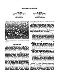
significant when we only have a small number of features. For a given number of features, the percentage of songs involved in constraints is augmented by five percent in each step, starting with 0 and stopping at 75. Its worth to note, that all experiments with random selection of songs to be constrained, have been run 10 times, and that all clustering evaluation measures are the means of these runs. In addition, a random base line clustering was used as a reference, where the items of each ground-truth class were randomly uniformly distributed over k estimated clusters. Resulting values of normalized mutual information are presented in Fig. 3. It is possible to note that the RAW scores tend to be more smooth over the incrementing size of the constrained set than scores for the outlier identification methods. Clustering results of LOF and RRS for small number of constraints – constrained data set smaller than 30% – from both Symmetric and Random Walk Laplacians are comparable to the clustering results with random constraints. On the other hand, for the high number of constraints and the high amount of features, the clustering results of both LOF and RRS and for both Laplacians are significantly better than clustering results with random constraints, bringing an improvement of up to 0.22 points of NMI. In fact, with more than 32 features the results are considerably better for almost all sets of constraints. Clustering with RRS seems to suffer from some instability, yet the differences between RRS an RAW with the Random Walk Laplacian are considerable while taking into account more than 32 features. We present the scores of clustering evaluation measures for all experiments in Fig. 2. As a representative example we look at the clustering results with 512 feature dimensions. Here the scores for Symmetric Laplacian with RAW and with LOF are considerably lower. On the other hand, the best results are obtained from RRS with both Random Walk and Symmetric Laplacians.
RESULTS
In this section we present the results for the experiments stated in Table 1 of Sec. 3. Each of the experiments is run over the following quantities of features: 16, 32, 64, 128, 256 and 512 determined through the powers of two. This log-line scale is used considering that improvement is more
In this paper we presented a system for the active exploration of music collections via spectral clustering with constraints. For the experiments we simulated the constraints through the ground-truth class labels of the audio genre dataset. Alongside with determining the constraint candidates in a random manner, we investigated two different outlier identification methods. Additionally we looked into a spectral feature selection method and proved the performance of clustering for two versions of Laplacian for spectral clustering.
7. ACKNOWLEDGMENT This work has been partly supported by the German research project GlobalMusic2One 2 funded by the Federal Ministry of Education and Research (BMBF-FKZ: 01/S08039B). Additionally, the Thuringian Ministry of Economy, Employment and Technology supported this research by granting funds of the European Fund for Regional Development to the project Songs2See 3 , enabling transnational cooperation between Thuringian companies and their partners from other European regions. 2 3
see http://www.globalmusic2one.net see http://www.songs2see.net
Symmetric Laplacian
Random Walk Laplacian
RAW
NMI
All
NMI NMI
Test
1
1
1
0.8
0.8
0.8
0.8
0.6
0.6
0.6
0.6
0.4
0.4
0.4
0.4
256
0.2
0.2
0.2
0.2
512
16 32 64 128
0
25
50
75
0
0
25
50
75
0
0
25
50
75
0
1
1
1
1
0.8
0.8
0.8
0.8
0.6
0.6
0.6
0.6
0.4
0.4
0.4
0.4
0.2
0.2
0.2
0.2
0
RRS
All
1
0
LOF
Test
0
25
50
75
0
0
25
50
75
0
0
25
50
75
0
1
1
1
1
0.8
0.8
0.8
0.8
0.6
0.6
0.6
0.6
0.4
0.4
0.4
0.4
0.2
0.2
0.2
0.2
0
0
25
50
75
0
0
25
50
75
0
0
25
50
75
0
RB 0
25
50
75
0
25
50
75
0
25
50
75
Percentage of dataset involved in constraints
Figure 3: Normalized Mutual Information (Y axis) versus the percentage of the dataset that is involved in at least one constraint (X axis), different number of selected features and different evaluated subsets (All data set and Test set). Each row is related to a particular outlier identification method. The two first columns are related to the Symmetric Laplacian and the following two columns to the Random Walk Laplacian. Results of columns 1 and 3 are related to the All data set, while columns 2 and 4 are related only to the Test data set.
Sym LOF
Sym RRS
RW LOF
1
0.8
0.8
0.8
0.6
0.6
0.6
0.2 0 0
Purity
1
0.4
0.4 0.2
25
50
0 0
75
25
50
0 0
75
0.8
0.8
0.8
0.2 0 0
Under−clustering
1
0.4
0.6 0.4 0.2
25
50
75
0 0
RB
0.2
1
0.6
RW RRS
0.4
1
Over−clustering
Pairwise F−measure
RW Raw
1
Accuracy
NMI
Sym Raw
25
50
25
50
75
25
50
75
0.6 0.4 0.2
75
0 0
Percentage of dataset involved in constraints
Figure 2: Values of several evaluation measures versus the percentage of the dataset that is involved in at least one constraint (X axis). Evaluation measures, starting from upper left plot and going to lower right plot: Normalized Mutual Information, Accuracy, Purity, Pairwise F-measure, Over-Clustering and UnderClustering. In each of these plots experiments presented in Table 1 are evaluated. The number of selected features is fixed to 512. Curves plotted with ‘crosses’ state for random baseline clustering.
8.
REFERENCES
[1] L. Atlas and S. S. Shamma. Joint acoustic and modulation frequency. EURASIP Journal on Applied Signal Processing, 2003:668–675, 2003. [2] J.-J. Aucouturier, B. Defreville, and F. Pachet. The bag-of-frames approach to audio pattern recognition: A sufficient model for urban soundscapes but not for polyphonic music. J. Acoust. Soc. Am., 122(2):881–891, 2007. [3] S. Basu, A. Banjeree, E. Mooney, A. Banerjee, and R. J. Mooney. Active semi-supervision for pairwise constrained clustering. In Proceedings of the 2004 SIAM International Conference on Data Mining (SDM-04), pages 333–344, 2004. [4] S. Basu, M. Bilenko, and R. J. Mooney. A probabilistic framework for semi-supervised clustering. In Proc. of the 10th ACM SIGKDD Int. Conf. on Knowledge Discovery and Data Mining (KDD), pages 59–68, 2004. [5] J. P. Bello and J. Pickens. A robust mid-level representation for harmonic content in music signals. In Proc. of the 6th Int. Conf. on Music Information
Retrieval (ISMIR), 2005. [6] M. M. Breunig, H.-P. Kriegel, R. T. Ng, and J. Sander. LOF: Identifying density-based local outliers. ACM SIGMOD Record, 29(2):93–104, June 2000. [7] C. Dittmar, C. Bastuck, and M. Gruhne. Novel mid-level audio features for music similarity. In Proc. of the Int. Conf. on Music Communication Science (ICOMCS), Sydney, Australia, 2007. [8] G. Gatzsche, M. Mehnert, D. Gatzsche, and K. Brandenburg. A symmetry based approach for musical tonality analysis. In Proc. of the 8th Int. Conf. on Music Information Retrieval (ISMIR), Vienna, Austria, 2007. [9] M. Gruhne and C. Dittmar. Comparison of harmonic mid-level representations for genre recognition. In Proc. of the 3rd Workshop on Learning the Semantics of Audio Signals (LSAS), Graz, Austria, 2009. [10] M. Gruhne, C. Dittmar, and D. Gaertner. Improving rhythmic similarity computation by beat histogram transformations. In Proc. of the 10th Int. Society for Music Information Retrieval Conf. (ISMIR), Kobe,
Japan, 2009. [11] B. Kulis, S. Basu, I. Dhillon, and R. Mooney. Semi-supervised graph clustering: a kernel approach. In Proc. of the 22nd Int. Conf. on Machine Learning (ICML), 2005. [12] K. Lee. Automatic chord recognition from audio using enhanced pitch class profile. In Proc. of the Int. Computer Music Conf. (ICMC), New Orleans, USA, 2006. [13] H. Lukashevich. Towards quantitative measures of evaluating song segmentation. In Proc. of the 9th Int. Conf. on Music Information Retrieval (ISMIR), pages 375–380, Philadelphia, USA, 2008. [14] U. Luxburg. A tutorial on spectral clustering. Statistics and Computing, 17(4):395–416, December 2007. [15] W. Peng, T. Li, and M. Ogihara. Music clustering with constraints. In Proc. of the 8th Int. Conf. on Music Information Retrieval (ISMIR), Vienna, Austria, 2007. [16] S. Ramaswamy, R. Rastogi, and K. Shim. Efficient algorithms for mining outliers from large data sets. In Proceedings of the 2000 ACM SIGMOD international conference on Management of data, pages 427–438, 2000. [17] M. Stein, B. M. Schubert, M. Gruhne, G. Gatzsche, and M. Mehnert. Evaluation and comparison of audio chroma feature extraction methods. In Proc. of the 126th AES Convention, Munich, Germany, 2009. [18] S. Stober and A. N¨ urnberger. A multi-focus zoomable interface for multi-facet exploration of music collections. In Proc. of the 7th Int. Symposium on Computer Music Modeling and Retrieval (CMMR), M´ alaga, Spain, 2010. [19] G. Tzanetakis and P. Cook. Musical genre classification of audio signals. IEEE Transactions on Speech and Audio Processing, 10(5):293–302, 2002. [20] C. Uhle, C. Dittmar, and T. Sporer. Extraction of drum tracks from polyphonic music using independent subspace analysis. In Proc. of the 4th Int. Symposium on Independent Component Analysis (ICA), Nara, Japan, 2003. [21] K. Wagstaff and C. Cardie. Clustering with instance-level constraints. In Proc. of the 17th Int. Conf. on Machine Learning (ICML), pages 1103–1110, 2000. [22] Z. Zhao and H. Liu. Spectral feature selection for supervised and unsupervised learning. In Proc. of the 24th Int. Conf. on Machine Learning (ICML), 2007.