Under various constraints, the hierarchical network architecture shows its advantages on sharing limited wireless channel bandwidth, balancing node energy.
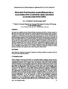
Applying Hierarchical Agglomerative Clustering to Wireless Sensor Networks Chung-Horng Lung, Chenjuan Zhou, Yuekang Yang Department of Systems and Computer Engineering Carleton University Ottawa, Ontario, Canada K1S 5B6 {chlung, cjzhou, yyang}@sce.carleton.ca Abstract Wireless Sensor Networks (WSNs) have a wide range of applications that base on the collaborative effort of a number of sensor nodes. Cluster-based network architecture can enhance network self-control capability and resource efficiency, and prolong the whole network lifetime. Thus, finding an effective and efficient way to generate clusters is an important topic in WSNs. Existing clustering approaches may not be flexible enough to cope with various factors or have higher communication overhead. To achieve the goal, we tailor the HAC (Hierarchical Agglomerative Clustering) algorithm for WSNs. HAC is a well-known approach and has been successfully applied to many disciplines. HAC uses simple numerical methods to make clustering decisions. In addition, HAC provides flexibility with respect to input data type (e.g., location data or connectivity information) and weight assignment to different factors (e.g., connections or power strength). This paper demonstrates our preliminary work in applying several well-understood HAC methods to WSNs. Initial results look promising. We are investigating other specific factors of WSNs, such as degree of connectivity, power level, and reliability, and are incorporating them into the HAC approaches.
1. Introduction In Wireless Sensor Networks (WSNs), a large number of sensor nodes could be deployed in various environments that cover large areas. These nodes sense environmental changes and collaborate to accomplish a common task such as environment monitoring or tracking. In many applications, sensor nodes must be self-organized because they usually are deployed in an infrastructureless network. Further, there are unique resource constraints and application requirements in WSNs, such as densely deployed nodes, extremely low power consumption, limited device capability, random topology, and etc [1]. Under various constraints, the hierarchical network architecture shows its advantages on sharing limited wireless channel bandwidth, balancing node energy consumption, reducing communication expense,
enhancing management, and so on [2]. In a hierarchical network, similar nodes aggregate into clusters. In each cluster, one node acts as a CH (Cluster Head) which is in charge of coordinating among the nodes within its cluster as well as communicating with other CHs. The cluster members just need to transmit messages to their CH. An effective and efficient approach to grouping nodes into clusters and selecting appropriate nodes to be the CHs is critically needed. Many clustering approaches have been proposed for WSNs. The existing approaches typically first select a set of CHs among the nodes in the network by considering one or multiple factors, and then gather the rest of the nodes under these CHs. LEACH [7, 8] is an important clustering protocol for WSNs as there are many approaches that are based on it. LEACH is fully distributed through randomly selecting CHs and rotating the CH task among nodes. Thus, the approach can uniformly distribute the energy consumption in the whole network. PEGASIS [9, 10] is based on LEACH and uses the greedy algorithm to organize all sensor nodes into a chain and then periodically promote the first node on the chain to be the CH. HEED [13] extends LEACH by initializing a probability for each node to be a tentative CH depending on its residual energy and making the decision according to the cost based on the connectivity degree of the node. These approaches have two main disadvantages. The first one is the random selection of the CHs, which may cause higher communication overhead for: (i) the ordinary member nodes in communicating with their corresponding CH, (ii) CHs in establishing the communication among them, or (iii) between a CH and a base station (BS) or other sinks. Another issue is the periodic CH rotation or election which needs extra energy to rebuild clusters. To avoid the problem of random CH selection, there are many other approaches focusing on how to select appropriate CHs to achieve efficient communications. Stojmenovic, et al. [11] proposed a dominating set algorithm which focuses on the efficiency of broadcasting to all the nodes. The approach divides all the nodes into four types: Gateway, Inter-Gateway, Intermediate and Member. The selected Gateway nodes which form a
dominating set ensure high efficiency of information transmission. However, the dominating set is breakable because any change to the network may cause the entire network to update and recalculate the dominate set again. Yin, et al. [12] proposed a novel cluster head selection algorithm using AHP (Analytical Hierarchy Process). The approach considers three factors: energy, mobility, and the distance to the involved cluster centroid. However, the sinks performing the algorithm introduces another issue that increases the communication cost between CHs and the sinks with the administration information. HAC (Hierarchical Agglomerative Clustering) [3, 6, 14] is a conceptually and mathematically simple clustering approach. In this paper, we advocate the HAC approach for WSNs. We will illustrate why and how to use the HAC approach to mitigate the problems encountered with current protocols. The following are the main advantages of the HAC approach: 1) Simple computation and easy implementation. Section 2 briefly illustrates this point. 2) Less restricted assumptions and more flexibility: HAC could use simple qualitative connectivity information of a network or quantitative data through Received Signal Strength (RSS) or GPS. In addition, other factors could easily be incorporated into the algorithm. For instance, different weights could be assigned to different nodes or connections for specific scenarios. 3) Less resource for clusters establishment: Using the HAC approach, nodes can finish the CHs election and announcement, cluster establishment, and scheduling at the same time. It can greatly reduce resource dissipation. 4) Without the need of periodic re-clustering or network updating: The HAC approach generates a logical CH backup chain during the cluster generation process. It makes clusters easily adaptive to network changes without extra information exchanges or the need of periodic announcement, such as CH. In the following, we will elaborate further on these advantages listed above. In section 2, we briefly introduce the concept of HAC algorithms. In Sections 3 and 4, we discuss the HAC design in WSNs. The original idea of HAC requires the global knowledge. In Section 3, we will start our discussion with the assumption that each node has the global information of every other node for concept illustration. Then we will remove the assumption by introducing the distributed method in Section 4. Finally, Section 5 is the conclusion.
2. HAC Concept Introduction This section presents the basis of HAC. Many different numerical taxonomy or HAC clustering techniques have been researched and proposed [3, 6, 14]. All of these approaches comprise three common key steps: obtain the data set, compute the resemblance coefficients, and execute the clustering method. For each step, there are various alternatives. For example, HAC has two important categories, divisive and agglomerative. Data types could be either quantitative or qualitative. Resemblance coefficient also has two types, dissimilarity coefficient and similarity coefficient. Our research does not focus on the clustering technique analysis and comparison. Instead, we will briefly describe the related concept of the HAC algorithms adopted in our research for WSNs and illustrate them with both quantitative and qualitative input data.
2.1. Input data set An input data set for HAC is a component-attribute data matrix. Components are the entities that we want to group based on their similarities. Attributes are the properties of the components. For example, the attributes could be the location of mobile nodes, the nodes’ residual energy, or other features. Figure 1 shows a simple randomly generated network. The components are the nodes and the attributes are their locations as illustrated in Table 1. We can easily add or remove components or attributes from the data set for different applications. Obviously, the more factors we consider, the more restricted assumptions and computations are needed.
Figure 1. A Simple 8-Node Network
Table 1. Component-Attribute Data Matrix for the 8Node Network Component (Node) 1 2 3 4 5 6 7 8
Attribute x-axis y-axis 3.78 2.9 3.56 4.83 6.06 7.34 7.71 8.46 0.63 0.01 7.23 5.78 8.52 3.46 4.43 0.48
2.2. Computation of resemblance coefficients A resemblance coefficient for a given pair of components indicates the degree of similarity or dissimilarity between these two components, depending on the way in which the data is represented. A resemblance coefficient could be quantitative or qualitative. Table 2 shows quantitative coefficients which measure the literal distance between two components when they are viewed as points in a two-dimensional array formed by the input attributes. The coefficients are calculated using the Euclidean distance based on the input data shown in Table 1.
2.3. Execution of the HAC method Execution of HAC usually has six steps; each step merges two clusters together and updates the Resemblance Matrix. Updating the Resemblance Matrix is an important step and various methods could be adopted. There are four main types of HAC [3]: 1) Single LINKage Algorithm (SLINK): also called the nearest neighbor method. Defines the similarity measure between two clusters as the maximum resemblance coefficient among all pair entities in the two clusters. 2) Complete LINKage Algorithm (CLINK): also called the furthest neighbor method. Defines the similarity measure between two clusters as the minimum resemblance coefficient among all pair entities in the two clusters. 3) Un-weighted Pair-Group Method using arithmetic Averages (UPGMA): Defines the similarity measure between two clusters as the arithmetic average of resemblance coefficients among all pair entities in the two clusters. UPGMA is the most commonly adopted clustering method in general. 4) Weighted Pair-Group Method using arithmetic Averages (WPGMA): Defines the similarity measure between two clusters as the simple arithmetic average of resemblance coefficients between two clusters without considering the cluster size.
Table 2. Resemblance Matrix with Quantitative Data 2 3 4 5 6 7 8 1 1.94 4.99 6.81 4.27 4.49 4.77 2.51 2 -3.54 5.51 5.64 3.79 5.15 4.44 3 --1.99 9.12 1.95 4.59 7.05 4 ---2.72 5.07 8.63 11 5 ----8.77 8.61 3.83 6 -----2.65 5.99 7 ------5.06 The simplest form of qualitative values is binary representation, e.g., the value is either 0 or 1. To deal with the qualitative input data, there are various ways to calculate the resemblance coefficients. Three typical methods are [3, 6, 14]: 1) Jaccard Coefficient: cxy = a / (a + b + c) 2) Simple Matching Coefficient: cxy = (a + d) / (a + b + c + d) 3) Sorenson Coefficient: cxy = 2a / (2a + b + c) where a, b, c, d are counts of 1-1, 1-0, 0-1, and 0-0 matches of attribute-pair between any two components x and y. An example is presented in Section 3.2.
Figure 2. Dendrograms Using Different HAC Methods
In HAC, the clustering result usually is represented with a dendrogram. In Figure 2, the height is the coefficient of between two merged components/clusters. Using the UPGMA approach (c), for instance, we can get two clusters (3,6,4,7) and (1,2,8,5) if a cut is selected right above the merger of node 5 and cluster (1,2,8). See Section 3.1 for further explanation. We can also see that, with the same data set, we may get different clustering results by using different HAC algorithms, e.g., (a) and (b).
3. Cluster Creation for WSNs HAC has been widely applied in many different areas [3, 6, 14]. Our research is to investigate the application of HAC in WSNs to set up clusters for communication efficiency. To illustrate the feasibility of HAC methods in WSNs, in this section, we start with the “best condition” which encompasses the following assumptions about the network:
between any pair of nodes. We can use the nodes transmission radius as the threshold to cut the cluster tree or determine clusters. The following steps and Figure 3 demonstrate how to generate the clusters and determine the CHs. Step 1: Execute HAC and get a cluster tree by using the UPGMA method. Step 2: Cut the cluster tree with the threshold of transmission radius. (The radius is 4. 38 for this example based on a calculation using the total number of nodes and average node degree, but could also be based on actual transmission capacity or an application specific pre-configured value. For brevity, it is not shown here.) As a result, three clusters, {3, 6, 4, 7}, {5}, {1, 2, 8} are generated, as shown in Step 2. Step 3: The size of cluster {5} is smaller than the Minimum_Cluster_Size; it is then combined with its closest cluster {1, 2, 8}.
1) 2) 3) 4)
The nodes in the network are quasi-stationary. Propagation channel is symmetric. Nodes are left unattended after deployment All nodes have similar capabilities, processing, communication and initial energy. 5) Each node has the global information of every other node. (This assumption will be removed in Section 4.) In WSNs, HAC is carried out in the clustering process as follows: 1) Nodes exchange messages until they obtain all of other nodes’ location information. 2) Run the clustering method and generate a cluster tree. 3) Make a cut using a pre-configured threshold value (e.g., transmission radius, number of clusters, or cluster density) to determine clusters. 4) If the cluster size is less than a pre-defined threshold, Minimum_Cluster_Size, merge the cluster with its closest cluster. 5) Once we finish clustering, CHs are initially determined by using the nodes which satisfy two conditions: (i) the node is one of two nodes which are merged into current cluster at the first step or the lowest level, e.g., (3, 6) or (1, 2) in Figure 2(b); (ii) the node with the lower ID. Another node which has the higher ID becomes the backup CH.
3.1. Application of HAC with quantitative
data To apply HAC with the quantitative data in WSNs, we have an assumption: nodes are location-aware. And hence, we use the location information to calculate the distance
Figure 3. Clustering Steps and Dendrogram Using UPGAM Algorithm with Quantitative Data Finally, we generate two clusters: {3, 6, 4, 7}, {1, 2, 8, 5} after Step 3. And at the same time, we can choose node 3 and node 1 as the CHs of these two clusters, since both are grouped with another node (nodes 6 and 2, respectively) in the first step and both have lower ID numbers. Those two clusters also correspond to the clustering sequence of the nodes in each cluster, which represents the cluster chain that can also be used for scheduling arrangement. For instance, cluster (3, 6, 4, 7)
demonstrates that the sequence of serving as the CH in this cluster is 3, 6, 4, and 7. Without any extra scheduling process, the CHs election and announcement, cluster establishment, and scheduling can be finished at the same time. The clustering sequence of the nodes in each cluster also can be used to handle the dynamic network conditions. If a node, e.g., node 3, can not be a CH anymore, the next node in the cluster chain, e.g., node 6, will be the new default CH without extra message exchanges due to the fact that each cluster member has the CH backup chain information. Similarly, if node 6 fails or becomes low in power, then the next node in the chain, node 4, will be the default CH. The decision of the scheduling policy can also be extended by considering the power level when an election of a CH is needed. In other words, node 4, for instance, may not have enough power. Node 4 in this case can simply elect the next node to be a CH even if it is the next node in the chain. With this mechanism, there is no need to re-execute clustering once we established clusters by using HAC.
instance, the parameters (see section 2.2.) and their values are a(1-1) = 3, b(1-0) = 0, c(0-1) = 0, d(0-0) = 5. We have experimented four different algorithms, SLINK, CLINK, UPGMA, and WPGMA, to calculate the resemblance coefficients and perform the clustering. Figure 4 shows the result of using the Sorenson algorithm (see section 2.2) to calculate the resemblance coefficients and the UPGMA for clustering computation.
3.2. Application of HAC with qualitative data To apply HAC with less information of nodes in WSNs, e.g., location information of nodes is not available, qualitative data can be adopted. In the absence of location information, the connectivity information can be used as input. Each node merely knows its neighbour list without distance or any other information. In other words, each connection can be represented with a binary value. In this paper, we use a 1 value to represent 1-hop connection and a 0 value to represent no direct connection. Hence, the input data for the 8-node network can be represented as follows: Table 3. 1-Hop Network Connectivity Data: a Partial Representation ID 1 2 3 4 5 6 7 8
1 1 1 0 0 1 0 0 1
2 1 1 1 0 0 1 0 0
3 0 1 1 1 0 1 0 0
4 0 0 1 1 0 1 0 0
5 1 0 0 0 1 0 0 1
6 0 1 1 1 0 1 1 0
7 0 0 0 0 0 1 1 0
8 1 0 0 0 1 0 0 1
Table 3 lists all 1-hop connections. Note that a 1 value is also used for a node to itself or the entries along the main diagonal to give more weight for the resemblance coefficient computation. Table 3 shows that node 1’s 1hop neighbours are (2, 5, 8). For nodes 5 and 8, for
Figure 4. Clustering Steps and Dendrogram for Qualitative Data Using Sorenson and UPGMA Methods The height value in Figure 4 is the Sorenson coefficient which indicates the similarity or closeness between two clusters. After using the threshold 0.5 to cut the cluster tree, the result shows that three clusters could be obtained. They are {3, 6, 4, 2}, {7}, and {5, 8, 1}. The size of Cluster {7} is smaller than the Minimum_Cluster_Size. We merge it with its closest cluster {3, 6, 4, 2}. Finally, we can get two clusters {3, 6, 4, 2, 7}, {5, 8, 1}, and node 3 and node 5 are the CHs. The result is similar to that obtained from using the quantitative data as presented in the previous section, except that node 2 is now in the other cluster. Node 2 is sitting in between two groups. It could be clustered with either group. Discrepancies in clustering results are common when different input data or clustering algorithms are used, since there are generally various ways to group data. The more important point is to group nodes that share more commonalities or are physically closer.
The main advantage of using the 1-hop connectivity information is that it can be easily obtained through message exchanges with low or no extra communication overhead. Our initial experiment shows that HAC with qualitative data could achieve good result with less information. We have experimented 2-hop neighbour knowledge in the clustering process and are currently evaluating further in this area. In addition, 1-hop neighbors and 2-hop neighbours could have different weights. We have conducted some preliminary experiments to consider both 1-hop and 2-hop connections with the same weight or different weights for several 20node and a 100-node networks. Several weight ratios between 1-hop and 2-hop connections have been evaluated, including 3:1, 2:1, and 8:3. The results in general are close. Further, our initial results also reveal that if we consider only the 1-hop information, we can have smaller number of clusters with the same threshold value. We are investigating further on this issue.
4. Distributed Clustering Algorithm
Without the global knowledge, we can make use of the neighbour information to determine if a node actually needs to perform the clustering task. The clustering could be conducted based on the location data or RSS. The rationale is that every node knows its 1-hop and 2-hop neighbours. If the neighbours of node x are a subset of node y’s neighbours, we can say node x is covered by node y. In this case, only node y needs to perform the clustering task due to its larger scope of neighbour information. Conceptually, the idea of coverage is similar to that presented by Stojmenovic, et al. [11]. u
v
w (a)
x
u
v
w (b)
x
y
u
v
w (c)
x
y
z
Figure 5. Network Topologies: an Illustration The results obtained by the clustering methods depicted in Section 3 looked promising. Some potential advantages include: (i) The CH election process is not periodic and the scheduling of CH within a cluster can generally follow the clustering chain. (ii) Each CH can effectively communicate with its members within the cluster, since battery power can be efficiently used within a certain transmission range. However, the assumption that each node has the global knowledge of all the nodes is not realistic for WSNs. In this section, we briefly describe how the clustering algorithm can be modified for distributed environments. The idea is that for WSNs, we do not actually need the global knowledge. Specifically, a node can make use of only neighbor knowledge, including both 1-hop and 2-hop neighbours for the computation. Nodes that are far apart will not be grouped into the same cluster anyway. Therefore, it is not necessary to include all the information for clustering. As a result, we can remove the assumption that each node has the global information of every other node. The following sections describe areas that are still work-in-progress. We are building and modifying tools to support effective analysis and evaluation. The rest of this section discusses the concept of distributed clustering for WSNs based on the quantitative location data and qualitative connectivity knowledge using the HAC approach.
4.1. Distributed clustering using quantitative
data
Figure 5 shows three simple network topologies. Each link represents a 1-hop connectivity. In other words, node u and node v are 1-hop away, but node u and node w are 2-hop neighbours. When each node is discovering its neighbours, it could also obtain the RSS or location information, if available, which will be used in the clustering process as demonstrated in Section 3.1. In Figure 5(a), either node v or node w have the broadest neighbour knowledge; therefore, either one can perform the clustering analysis. In (b), every node is covered by w. Hence, clustering only needs to be conducted by node w. In (c), both node w and node x need to run the clustering method, because they have different neighbour information. This will typically result in different clustering results for node w and node x. The result obtained from node w in Figure 5(c) will be used to identify clusters for node u, node v, and node w only. On the other hand, the result computed by node x is only locally meaningful but sufficient to node x, node y, and node z. Figure 6 shows the pseudo code of the distributed HAC implementation for WSNs. In the beginning, each cluster exchanges the neighbor information with its neighbors. Lines 1-4 initialize the clustering process. Under the predefined threshold, the while loop in lines 5-15 control the size of clusters. During the clustering process, all clusters keep listening and waiting for Invite messages (lines 6-9). After receiving the Invite messages, any two matched clusters merged together as a new cluster (line 10-11, lines 16-22). The CH of the new cluster broadcasts
an Inform message to notify their neighbours to update the Resemblance matrices (lines 13, 14). The Inform message includes the new cluster information and the combined neighbour list. At every cluster merging step, clusters can update their Resemblance matrices by exchanging their neighbor information, without relying on global information. /* A cluster sets up the Resemblance matrix by using the collected information. */ /* Initialization */ 1. find the minimum in the Resemblance matrix, MinV, Let MinC be the cluster ID corresponding to MinV; 2. if (isCoveredbyMinC==False) 3. send an Invite message to cluster MinC; 4. endif /* Clustering*/ 5. while (MinV