A brief survey of unsupervised agglomerative hierarchical clustering

International Journal of Engineering & Technology, 8 (1) (2019) 29-37

International Journal of Engineering & Technology Website: www.sciencepubco.com/index.php/IJET doi: 13791 Research paper

A brief survey of unsupervised agglomerative hierarchical clustering schemes Sreedhar Kumar S 1 *, Madheswaran M 2, Vinutha B A 1, Manjunatha Singh H 1, Charan K V 1 1 Department

of CSE, Dr. T Thimmaiah Institute of Technology, Kolar Gold Field, Karnataka-563120, India of ECE, Mahendra Engineering College, Namakkal Dt.-637503, Tamilnadu, India *Corresponding author E-mail: [email protected]

2 Department

Abstract Unsupervised hierarchical clustering process is a mathematical model or exploratory tool aims to provide the easiest way to categorize the distinct groups over the large volume of real time observations or dataset in tree form based on nature of similarity measures without prior knowledge. Dataset is an important aspect in the hierarchical clustering process that denotes the behavior of living species depicts the properties of a natural phenomenon and result of a scientific experiment and observation of a running machinery system without label identification. The hierarchical clustering scheme consists of Agglomerative and Divisive that is applicable to employ into various scientific research areas like machine learning, pattern recognition, big data analysis, image pixel classification, information retrieval, and bioinformatics for distinct patterns identification. This paper discovered a brief survey of agglomerative hierarchical clustering schemes with its clustering procedures, linkage metrics, complexity analysis, key issues and development of AHC scheme. Keywords: Agglomerative Hierarchical Clustering; Clustering Process; Distance Metric; Divisive Hierarchical Clustering; Similarity Measure; Linkage Method.

1. Introduction Unsupervised hierarchical clustering technique is an oldest clustering scheme and is utilized to identify the finite number of dissimilar clusters over the dataset in hierarchy manner based on data objects similarity. The result of the hierarchical clustering scheme is represented in the form of binary tree structure or dendrogram. Basically, it consists of two types Divisive Hierarchical Clustering (DHC) and Agglomerative Hierarchical Clustering (AHC). In DHC is a top-down method, it starts with n data objects in single large cluster and recursively n splitting the cluster into n smaller clusters with single data object and it requires higher computational cost O(2 ) (Athman et al 2015) [2]. Similarly, the AHC is a bottom-up method that starts with n clusters, each of which includes exactly one object (William et al 1984). It recursively partitions the dataset into a tree structure through a series of merge operations based on proximity measures. And finally, it forces all the clusters into a single cluster. Many authors suggested according to the clustering performance of hierarchical clustering based on several parameters that is the AHC scheme consumes lower computational cost compare to DHC method. The merge operation is an important process in the AHC technique that is used to find the closest cluster pair with a minimum distance and merged into single cluster based on clustering linkage method (Lance & Williams 1967) [24]. The clustering linkage method computes the distance between the two closest clusters with a set of object pairs and is classified into several types, namely Single Linkage (SLINK) [19], [21], [36], [35], Complete Linkage (CLINK) (Defays 1977) [8], Unweighted Pair Group Method with Arithmetic Mean (UPGMA) or Average Linkage [19], [51], Weighted Average Linkage or Weighted Pair Group Method Average (WPGMA) [19], [29], Centroid Linkage or Unweighted Pair Group Method Centroid (UPGMC) [37], Median Linkage [15], [16], Wards Method (Ward 1963) [42] and Pair-wise Nearest Neighbor [4], [12], [30].

2. Traditional AHC scheme AHC is a one of the powerful traditional unsupervised hierarchical clustering method, it intentions to separate the distinct clusters over the large data points based on nature of similarity in sequence of merging operations without prior knowledge.

2.1. AHC procedure Generally, the AHC start with n individual clusters with single data object as defined X = xi for i = 0,1,.., n , where X denotes the dataset or cluster set, x i represents the i th cluster or data object in cluster set X and n is the size of dataset or cluster set X . Next, it Copyright © 2019 Sreedhar Kumar S et al. This is an open access article distributed under the Creative Commons Attribution License, which permits unrestricted use, distribution, and reproduction in any medium, provided the original work is properly cited.

30

International Journal of Engineering & Technology

construct the distance matrix D(X ) for cluster set or dataset X with matrix size of ( n n ) based on distance metrics such as Euclidean, Square Euclidean, Manhattan, Hamming, Maximum [47, 48, 51] and is defined as

  D( X ) = d ( xi , x j ) xi , x j  X    i , j = 0,1,..,n

(1)

th Where d ( xi , x j ) denotes the similarity distance (Euclidean) between i th and j clusters and is defined as.

d ( xi , x j ) =

 (x − x )  2

i

(2)

j

Next, it finds the closest cluster pair ( xi , x j ) with minimum distance (higher similarity) mdij over the distance matrix D(X ) for i = 0,1,.., n − 1 and j = 0,1,.., n − 1 where mdij denotes the minimum distance of closest cluster pair ( xi , x j ) and is defined as

D( X )   mdij =   i, j = 0,.., n − 1

(3)

Afterward, it merges the closest cluster pair x i and x j into single cluster x i and update the number of objects in the merge cluster x i and is defined as

Ni = Ni  N j

(4)

Here, Ni and N j represent the number of data objects in the respective

xi

and

xj

th clusters. Next, the AHC deletes the j cluster x j

in the cluster set X and update the cluster set size by

n = n −1

(5)

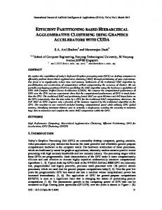
Where n denotes the number of clusters in cluster set or size of dataset X . Repeat the above procedures until all the clusters in the cluster set forced into the single large cluster with cluster set size n is equal to one. At the every iteration, the AHC is merging two closest clusters only with higher similarity. Figure 1 show various steps involved in the AHC method. In the other hand, after two iterations in the clustering process that the clusters size could increase. If the clusters have more than one data objects, then use the linkage metric and compute the distance between the clusters. The linkage metric and distance measure are major aspects in the AHC scheme that discussed in the following subsections. The traditional AHC algorithm has described in the below subsection.

2.2. AHC algorithm Input: Dataset X = x0 , x1,.., n with n data objects Begin 1) Define each data object is an individual cluster in dataset X for i = 0,1,.., n 2) REPEAT a) Built distance matrix D(X ) for input cluster set X by Equation (1) b) Find closest cluster pair ( xi , x j ) over the D(X ) with minimum distance to be merged into single cluster xi  x j → xij → xi by c) d) e) 3) End

Equation (3) Update the merged cluster size by Equation (4) th

Delete the j cluster in X Reduce the cluster set size by one. UNTIL n = 1

International Journal of Engineering & Technology

31

Fig. 1: Functional Diagram of Traditional AHC Scheme.

3. Various linkage metrics Linkage metric is a most impotent process in the AHC clustering scheme and it aims to compute distance between two clusters x i and x j with more than one data objects ( Ni , N j  1 ), where Ni and N j represent the number of data objects in the respective x i and x j clusters in X . There are many traditional linkage metrics have reported in past decades to improve the clustering performance of AHC scheme like SLINK, CLINK, UPGMA, WPGMA, UPGMC, Median Linkage, Ward’s and PNN. The linkage metrics are discussed in the below subsections.

3.1. Slink The single linkage (SLINK) [36, 49] method is employed for grouping clusters in bottom-up fashion, which, at each step, combines two clusters that enclose the closest pair of objects not belonging to the same cluster as each other. It consists of two steps, in the first step, it computes the distance of object pairs between two clusters x i and x j with more than one data objects. In the next step, it discovery the distance of cluster pair x i and x j by finding the minimum distance among the distance of object pairs xi = xir for r = 0,1,.., Ni and

x j = x je for r = 0,1,.., Ni between i th and j th clusters and is defined as    xir  xi ,    d ( xi , x j ) = mind ( xir , x je ) x je  x j ,   r =0,1,..,N i   e =0,1,..,N j xi , x j  X    Where d ( xir , x je ) denotes the similarity distance (Euclidean) of r the i

th

(6)

th

and e

th

object between i

th

and j th clusters, x i and x j represent

and j th clusters with number of objects N i and N j respectively.

3.2. Clink Another type of agglomerative clustering is called complete linkage (CLINK) [50] method. In this method, initially, each object is in a cluster of its own and the clusters are serially combined into larger clusters until all the data objects integrated within the same cluster. At each step, two clusters that are separated by the shortest distance are combined. First, it calculates the similarity distance among the every individual object pairs between two clusters x i and x j based on distance measure (Euclidean). Next, it search the distance of cluster pair

32

International Journal of Engineering & Technology

x i and x j by finding the maximum distance among the distance of object pairs xi = xir for r = 0,1,..,Ni and x j = x je for r = 0,1,..,Ni between i th and j th clusters and is defined in the Equation (7) as   x ir  x i ,  d ( x i , x j ) = maxd ( x ir , x je ) x je  x j ,  r =0,1,..,N i  e =0,1,..,N j x i , x j  X 

      

(7)

3.3. Average linkage A simple agglomerative hierarchical clustering method called group average linkage or Unweighted Pair Group Method with Arithmetic Mean (UPGMA) [51]. It paradigms an entrenched tree to replicate the structure present in a pair wise similarity matrix. At the every iteration, the closest two clusters are joint into a higher level cluster. The distance between any two clusters x i and x j is taken to be the average of all the distances between pairs of, that is, the mean distance between elements of each cluster and is defined as

 x ir  x i ,     1  d ( xi , x j ) =   d ( x ir , x je ) x je  x j ,  N  N j r =0 e =0  i  xi , x j  X    



(8)

Similarly, to calculate the distance between the merged cluster xi , j and a new cluster x l is defined as

((

) )

d xi , x j , xl =

(

Ni  d (xi , xl ) + N j  d x j , xl

)

(9)

Ni + N j

3.4. Weighted average linkage The weighted average linkage method is called Weighted Pair Group Method Average (WPGMA) [29]. The WPGMA is similar to UPGMA scheme, but the difference is that the distances between the newly constructed cluster and the rest are weighted based on the number of data objects in each cluster. Initially, it computes the distance of each individual object pair among the clusters x i and x j based on distance measure (Euclidean). Next, it calculates distance between two clusters x i and x j by finding average of distance of object pairs among the cluster pair and is defined in the Equation (7) as

 x ir  x i ,  1 2 d ( xi , x j ) =   d ( x ir , x je ) x je  x j ,  2 r =1 e =0 xi , x j  X 



    

(10)

In the other way to calculate the distance between the two clusters ( xi  xk ) and x j by

(

)

d xi , k , x j =

(

) (

d xi , x j + d xk , x j

)

(11)

2

3.5. Centroid & median linkages Centroid linkage method is also called Unweighted Pair Group Method Centroid (UPGMC) [37]. This method merges the two closest clusters into single cluster based on distance between the centroids of the each individual cluster and it could be represented as

(

)

d xi , x j = ci − c j

2

(12)

Where c i and c i denote the centroid of the individual clusters x i and x j respectively, ci − c j is the Squared Euclidean distance between centroids of cluster pair xi , j and is defined by Ni

ci =

x

ie

e −1

Ni

(13)

International Journal of Engineering & Technology

33

Next, the median linkage method is also called Weighted Pair Group Method Centroid (WPGMC) [15, 16]. This scheme is almost equivalent to (UPGMC) method, except that the equal weight is given to the clusters to be merged. It computes the distance among the merged cluster xi , j and new clusters x k and is defined in the Equation (14) as.

(

d xi, j , x k

)

(

1 1  2 d (x i , x k ) + 2 d x j , x k = − 1 d x , x i j  4

(

)

)   

(14)

3.6. Wards method Ward’s method is also called Minimum Variance Method (MVM), and its objective is to reduce the sum of squared errors among individual clusters. It measures the distance among the cluster pair in two ways. In the first way, it estimates the distance between two individual clusters xi , x j with single data object based on Squared Euclidean and is defined as

(

(

)

)

d xi , k , x j = xi − x j

2

(15)

(

)

Another way it calculates the distance between merged cluster xi  x j and new cluster x k based on Lance-William method and is defined as

 Ni + N k  d (xi , xk ) +   N + N + N j k  i   N +N    j k d xi , j , xk =  d x j , xk  N + N + N j k  i    Nk − d xi , x j   N i + N j + N k 

(

)

(

)

(

(16)

)

th Where, x i , j denotes the newly merged cluster and N i , N j and N k represent the size of the clusters i , j

th

and k

th

respectively.

3.7. Pairwise nearest neighbor Pairwise Nearest Neighbor (PNN) scheme (Chih-Tang et al. 2010) [4] is a type of agglomerative clustering method and it generates hierarchical clustering using a sequence of merge operations until a desired number of clusters are obtained. The PNN method computes the distance between two clusters d ( xi , x j ) with more than one data objects and is defined as d ( xi , x j ) =

Ni N j Ni + N j

 d ( xi , x j )

(17)

th Where, xi and x j represent the centers (mean) of i and j th clusters respectively, d ( xi , x j ) denotes the distance between centers of

cluster pair ( xi , x j ) . The selected cluster pair x i and x j is to be merged into single cluster xi , j → xi and then update the merged cluster x i center xi , j → xi by

xi =

Ni xi + N j x j Ni + N j

(18)

The size of the merged cluster Ni , j → Ni is updated by Ni = Ni + N j

(19)

3.7. Complexity analysis A detailed computational complexity analysis of traditional AHC (bottom-up approach) is discussed. At the first iteration, the AHC scheme consumes  n 2 time to construct the distance matrix D(X ) with memory size of ( n  n) , where n denotes the number of data objects

( )

or clusters and X represents the dataset or cluster set as X = xi for i = 0,1,..,n . Next, for searching the AHC is required (n 2 ) time to trace the closest clusters pair ( xi , x j ) with minimum distance md ij over the distance matrix D(X ) for i = 0,1,..,n − 1 , j = 0,1,..,n − 1where

i and

j

represent the clusters x i and x j respectively. Then, it requires constant time to merge the closest clusters pair x i and x j into

34

International Journal of Engineering & Technology

single cluster x i . Within the same iteration, the updating process requires O(n) time to eliminate j th cluster in the cluster set X and respectively modify the newly constructed cluster x i size and cluster set X size. Finally, the AHC (bottom-up) is required O(n2 ) for both space and computational complexity to merge the two closest clusters at single iteration. Therefore, the traditional AHC scheme is required overall space and computational complexity of O(n3 ) for (n − 1) iterations. Therefore, there is a chance to reduce the AHC complexity cost from O(n3 ) into O(n2 lon n) , assume that the AHC is utilizing the heap structure to search the minimum distance of cluster pair over the distance matrix [33].

3.8. Major issuses of AHC scheme Several drawbacks that affect the performance of the traditional AHC (bottom-up) approachs that discussed by many of authors (Sudipto et al. 2000; Sudipto et al. 2001; Manoranjan et al 2003; Pasi et al 2006; Lai et al 2011; Athman et al 2015; De Amorim 2015) and reported in [2], [7], [23], [26], [33], [38], [39] include, the following: 1) Higher computational requirement to merge the two closest clusters by linkage methods (single, complete, average, weighted, centroid, median and wards) 2) Consumption of (n-1) iterations to categorize large dataset in tree structure where n denotes the number of data objects 3) Every iteration require O n 2 memory space to construct distance matrix and need O(n 2 ) time to search and merge the closest cluster pair 4) Consumption of high space and computational complexity O(n 3 ) for (n − 1) iterations. 5) Difficulties to find the optimum number of finest clusters over the single clustering tree with (n − 1) levels 6) Validation method is inefficient and inaccurate for evaluating the clustering result over the (n − 1) levels 7) It is not well suitable to process the large volume of dataset and mixed type of dataset due to the higher space and computational cost. 8) It filed to robotically produce finest number of dissimilar cluster over the dataset without pre determining number of clusters. 9) It is not well comfortable to process the categorical dataset, mixed type dataset, large document, image and video.

( )

4. Discussion of AHC development In the past years, many of the authors presented different hierarchical clustering schemes to improve the performance and reduced the space and computational cost of traditional AHC (bottom-up) technique, namely Balance Iterative Reducing and Clustering using Hierarchical (BIRCH) (Zhang et al. 1996) [44], CHAMELEON (George et al. 1999) [13], Fast Pairwise Nearest Neighbor (FPNN) (Franti et al 2000) [12], Fast Hierarchical Agglomerative Clustering (FHAC) (Manoranjan et al 2003) [26], K-Nearest Neighbor Graph (KNNG) (Pasi et al 2006) [33], Dynamic K-Nearest Neighbor Algorithm (DKNNA) (Lai et al 2011) [22], K-means and Agglomerative (KnA) (Athman et al 2015) [2, 52] and so on. BIRCH is an important hierarchical clustering technique that is used to process the very large scale dataset [44]. Initially, the BIRCH scheme constructs the Clustering Feature (CF) tree over the entire dataset based on height-balanced tree. Each leaf of CF tree has containing sufficient summaries of actual data objects or sub cluster. Next, it rebuilds the smaller CF tree by scanning all the leaf in the initial CF tree. Finally, it clusters the all leaf entries or sub clusters based on existing agglomerative clustering scheme. During the CF tree construction, the outliers are eliminated from the summaries through identifying the objects sparsely distributed in the feature space. The major achievement of this technique is claimed that it reduces computational complexity from O (n 3 ) into O (n ) to process the very large scale of dataset within the limited memory space. George et al. (1999) [13] have designed a cluster based outlier detection method called CHAMELEON. This approach identifies normal clusters and outliers on the dataset based on three steps. In the first step, it constructs the k-nearest neighbor graph over the entire dataset based on distance metrics. Next, it uses a graph partitioned algorithm that aimed to divide the dataset into several relatively small sub graphs or clusters and in the last step, it identifies the desired distinct clusters and outliers through the process of repeatedly merging the small clusters. The authors claimed that the CHAMELEON method is reduced the overall computational cost from O(n3 ) into O (n 2 ) for clustering the large dataset, where n denotes the number of data objects. The authors Franti et al (2010) [12] have presented another form of agglomerative clustering scheme namely Fast Pairwise Nearest Neighbor (FPNN) that intended to reduce the computational cost of existing PNN method from O (n 3 ) into O ( n 2 ) , where n denotes the number of data objects and  represents the average number of clusters to be merged. Initially, it traces nearest neighbor objects of each individual data object in the dataset and subsequently it maintains the nearest neighbor status of each object into nearest neighbor table. Then, it traces the closest cluster pair with minimum distance to be merged into single cluster. Afterward, it updates the centroid, size and nearest neighbor table status of newly merged cluster. Repeat the steps until to get the desired m distinct clusters in the final output, where m indicates the number of distinct clusters. Manoranjan et al. (2003) [26] have reported a Fast Hierarchical Agglomerative Clustering (FHAC) scheme which is based on Partially Overlapping Partitioning (POP). It consists of two-phases. In the first phase, large numbers of closest small clusters are merged based on POP method and in the second phase, the remaining small numbers of larger clusters are merged when the closest cluster pair distance exceeds the separating distance. The advantage of this algorithm is that it reduces the overall computation cost from O (n 3 ) into O (n 2 log n ) for clustering the large dataset. Similarly, Vijaya et al. (2004) [41] have reported another hierarchical clustering technique called Leaders Sub Leaders for large datasets. It uses an incremental clustering principle that intentions to generate a hierarchical structure for identifying the sub-clusters within each cluster. Szekely et al. (2005) [40] also have reported a hierarchical clustering method to minimize the joint between within measures of distance between clusters. It is an extension of Ward’s minimum variance method to identify clusters with nearly equal centers. Lin and Chen (2005) [25] have reported a two phase clustering algorithm called Cohesion based Self Merging (CSM). First phase, it partitions the input dataset into several small sub- clusters and in the second phase, it continuously combines the sub clusters into desired number of dissimilar clusters based on cohesion in a hierarchical way. The CSM approach is claimed to be robust and it possesses excellent tolerance to outlier in various datasets.

International Journal of Engineering & Technology

35

Pasi et al. (2006) [33] have presented another type of fast agglomerative clustering method using an approximate nearest neighbor graph to reduce the number of distance calculations. It starts by constructing a neighborhood graph in the first step and then iteratively merges pairs of clusters until the desired numbers of clusters are obtained. The advantage of this method is that it reduces time complexity for every search from O (n ) to O (k ) where, n is the number of data objects and k represents the number of centroid clusters. Weakness of this method is that the parameter k affects the quality of the clustering result and running time. Chung-Chain et al. (2007) [5], a distance hierarchy scheme for both categorical and numerical value which is reported as an integrated scheme for agglomerative hierarchical clustering with mixed data. It supports to estimate similarity relationships between categorical values and hence produces better clustering results. Hisashi Koga et al. (2007) [18] have reported a fast approximation algorithm for single linkage method that reduced the time complexity by rapidly finding the nearest clusters to be connected by Locality Sensitive Hashing (LSH). This method is faster and better than the single linkage method and at the same time, the authors suggest that the result of the scheme is almost similar to single linkage approach. Another technique called agglomerative fuzzy K-Means clustering algorithm is reported by Mark et al. (2008) [27] for numerical data to determine the number of clusters. This scheme follows penalty term procedure to the objective function to make the clustering process in sensitive to the initial cluster centers. It is further claimed that this approach could produce consistent clustering and determines the correct number of clusters in different datasets. Antti Honkela et al. (2008) [1] reported two variants of an agglomerative technique to learn a hierarchy of independent variable of group analysis. It is similar to hierarchical clustering, but the choice of clusters to merge is based on a variation Bayesian model comparison. In addition, it determines optimal cutoff points in the hierarchy. Caiming et al. (2011) [3] reported a split and merge hierarchical clustering method based on Minimum Spanning Tree (MST) graph. The MST based graph is used to control the splitting and merging process. In the splitting stage, it constructs the MST graph over the dataset with n objects and then it split the MST graph into sub graphs or sub clusters based on K-means technique. Next, in the merging stage, it iteratively joins the closest sub graphs or clusters into desired number of k distinct clusters based on nearest neighbor merging method. Finally, this scheme is reduced the computational cost from O (n 3 ) into O (n 2 f ) where f denotes the number of features in data object. The drawback of this method is that the universality of the definitions of inter-connectivity and inter-similarity are insufficient. Similarly, the authors Lai et al. (2011) [23] presented another improved agglomerative clustering algorithm namely Dynamic K-Nearest Neighbor Algorithm (DKNNA) to reduce the number of distance calculations and time complexity. Generally, the DKNNA scheme is similar to original version of Ward’s method and it used to identify the distinct number of dissimilar clusters based on k-nearest neighbor list within limited memory. The advantage of this approach is that it is faster and simultaneously it produces better clustering results with lower computational cost O (n 2 ) compared to Double Linked Algorithm (DLA) and Fast Pair-wise Nearest Neighbor (FPNN) techniques. Fionn & Legendre (2014) [11] reported a general agglomerative clustering technique with minimum variance method, where each step finds a pair of clusters that lead to minimum increase in total within-cluster variance after merging. This increase is the weighted square distance between cluster centers. Recently, Athman et al. (2015) [2] designed an integrated clustering approach called K-means and agglomerative (KnA) to reduce the computational complexity of traditional agglomerative scheme based on group of centroids. In the first stage, it partitions the dataset into k distinct clusters based on K-means scheme, then it computes the centroid of each individual cluster in the result of K-means. Second stage, the KnA scheme identifies the m dissimilar clusters over the centroids of k groups instead of raw data objects based on traditional agglomerative clustering methods (SLINK or CLINK), where m denotes the number of clusters. It follows a k group of centroids instead of raw data points to build cluster hierarchies, where centroid is indicated as a group of adjacent points in the data space. Finally, the authors claimed based on comprehensive experimental study that this approach reduces the computational cost from O (n 3 ) into O (nk + k 3 ) without compromising clustering performance, where k denotes the number of centroids, n is the number of raw data points. Another scheme, Nearest Neighbor Boundary (NNB) reduces the time and space complexity of standard agglomerative hierarchical clustering based on nearest neighbor search and it is designed by Wei et al. (2015) [43]. In the first step, it splits the dataset into independent sub regions and then it identifies the closest data objects over the each individual sub region and join together based on nearest neighbor search. In the next step, it traces the closest data objects among the sub regions or subset and joins together based on nearest neighbor boundary search. The merit of this method is that it consumes lower space and computational complexity O (n log2 n ) for grouping the nearest data points. A different clustering scheme called improved Limited Iteration Agglomerative Clustering (iLIAC) was reported by Krishnamoorthy and Sreedhar Kumar (2016) in [45]. This scheme uses to automatically separate optimum number of dissimilar clusters and outliers on large dataset based on optimum merge cost. First stage, it computes the optimum merge cost over the dataset based on statistical variance. Next, it traces supreme number of dissimilar clusters through iteratively builds the upper triangular distance matrix and finds closest data objects with minimum distance to be merged until the minimum distance of cluster pair exceed the optimum merge cost. The space complexity is reduced from O (n 2 ) into O  n  for n  (n 2 2)  n 2 to construct the upper triangular distance matrix instead of distance matrix. Finally it 2

 2 

reduced the overall computational cost from O (n 3 ) into

n  O   2  3

for (n − k ) iterations, where k denotes the number of distinct clusters that

identified automatically. Similarly another improved agglomerative clustering scheme namely Dynamic Automatic Agglomerative Clustering (DAAC) was designed by Madheswaran & Sreedhar kumar (2017) in [46] to identify best number of dissimilar clusters over the two dimensional dataset based on sum (count) of representative objects without prior knowledge. Initially, the DAAC finds the sum ( K ) of representative objects over the two dimensional dataset robotically by tracing rate of occurrences (number of neighbors) of each individual objects in dataset based on Euclidean distance, where K denotes the number of dissimilar objects. Then, it identifies the distinct representative objects based on rate of occurrence of data objects. In the clustering stage, the DAAC scheme iteratively identifies highly relative dissimilar clusters over the spatial two dimensional dataset until the number of clusters equal to count ( K ) of representative objects based on sequence of merging process. In the every iteration, the DAAC scheme is reduced space and computational cost through constructing upper triangular distance matrix for dataset and subsequently it computes the centroid of newly merged clusters. The authors climbed that the DAAC approach is produced appropriate number of dissimilar clusters with lesser computational cost compared to traditional AHC.

36

International Journal of Engineering & Technology

5. Summary This paper presents detail survey of agglomerative hierarchical clustering schemes. Firstly, we provided investigation status of clustering procedures, complexity analysis and key issues over the traditional AHC schemes like SLINK, CLINK, UPGMA, WPGMA, UPGMC, Median Linkage, Ward’s and PNN. We understood the AHC scheme through the investigation that it is the oldest hierarchical clustering method and its performance is limited by many factors such as higher computational cost for merging closest groups, required n-1 iterations, failed to automatically separate distinct clusters over the large dataset and so on. Similarly, we have discussed briefly about the development of AHC method through recently reported some important schemes namely BIRCH, CHAMELEON, FPNN, FHAC, DKNNA, KnA and so on. Based on the deep survey, we here by conclude that the major issues of the traditional AHC scheme are dissolved and subsequently the AHC scheme is well improved to employ into many scientific applications to identify distinct clusters over the big data such as large scale mixed dataset, document, image and video for analysis and decision making.

References [1] Antti Honkela, Jeremias Seppa & Esa Alhoniemi, “Agglomerative independent variable group analysis”, Neurocomputing, vol. 71, 2008, pp. 1311-1320. https://doi.org/10.1016/j.neucom.2007.11.024. [2] Athman Bauguettaya, Qi Yu, Xumin Liu, Xiangmin Zhou & Andy Song, “Efficient Agglomerative Hierarchical Clustering”, Expert Systems with Applications, vol. 42, no. 5, 2015, pp. 2785-2797. https://doi.org/10.1016/j.eswa.2014.09.054. [3] Caiming Zhong, Duoqian Miao & Pasi Franti, “Minimum Spanning tree based split-and-merge: A hierarchical clustering method”, Information Sciences, vol. 181, 2011, pp. 3397-3410. [4] Chih-Tang Chang, Lai Jim, ZC & Jeng, MD, “Fast agglomerative clustering using information of k-nearest neighbors”, Pattern Recognition, vol. 43, 2010, pp. 3958-3968. https://doi.org/10.1016/j.patcog.2010.06.021. [5] Chung-Chain Hsu, Chin-Long Chen & Yu-Wei Su, “Hierarchical clustering of mixed data based on distance hierarchy”, Information Sciences, vol. 177, no. 20, 2007, pp. 4474-4492. https://doi.org/10.1016/j.ins.2007.05.003. [6] Davies, DL & Bouldin, DW, “Cluster Separation Measure”, IEEE Transaction on Pattern Analysis and Machine Intelligence, vol. 1, no. 2, 1979, pp. 95-105. https://doi.org/10.1109/TPAMI.1979.4766909. [7] De Amorim, RC, “Feature Relevance in Ward”s Hierarchical Clustering Using the Lp Norm”, Journal of Classification, vol. 32, no. 1, 2015, pp. 46–62. https://doi.org/10.1007/s00357-015-9167-1. [8] Defays, D, “An efficient algorithm for a complete link method“, Computer Journal British Computer Society, vol. 20, no. 4, 1977, pp. 364–366. https://doi.org/10.1093/comjnl/20.4.364. [9] Duda, R, Hart, PE & Stork, DG, “Pattern classification”, 2nd edition, New York, NY: John Wiley & Sons, 2001. [10] Dutta, M, Kakoti Mahanta, A & Arun Pujari, K, “QROCK: A quick version of the algorithm for clustering of categorical data”, Pattern Recognition Letter, vol.26, 2005, pp. 2364-2373. https://doi.org/10.1016/j.patrec.2005.04.008. [11] Fionn Murtagh & Legendre P, “Wards hierarchical agglomerative clustering method: which algorithms implement wards criterion”, Journal of Classification, vol. 31, 2014, pp. 274-295. https://doi.org/10.1007/s00357-014-9161-z. [12] Franti, P, Kaukoranta, T, Sen, DF & Chang, KS, “Fast and memory efficient implementation of the exact PNN”, IEEE Transaction on Image Processing, vol. 9, 2000, pp. 773-777. https://doi.org/10.1109/83.841516. [13] George Karypis, Eui-Hong Han & Vipin Kumar, “Chameleon: Hierarchical Clustering Using Dynamic Modeling, Computers”, vol. 32, no. 8, 1999, pp. 6875. https://doi.org/10.1109/2.781637. [14] George Kollios, Dimitrios Gunopulos, Nick Koudas & Stefan Berchtold, “Efficient Biased Sampling for Approximate Clustering and Outlier Detection in Large Data Sets”, IEEE Transaction on Knowledge and Data Engineering, vol. 15, no. 5, 2003, pp. 1170-1187. https://doi.org/10.1109/TKDE.2003.1232271. [15] Gower J, “A comparison of some methods of cluster analysis”, Biometrics, vol. 23, no. 4, 1967, pp. 623-628. https://doi.org/10.2307/2528417. [16] Gower, JC & Ross, GJS, “Minimum spanning trees and single linkage cluster analysis”, Journal of the Royal Statistical Society, Series C, vol. 18, no. 1, 1969, pp. 54–64. https://doi.org/10.2307/2346439. [17] Ham, J & Kamber, M, “Data Mining: Concepts and Techniques”, 2nd Edition. Kaufmann, 2006. [18] Hisashi Koga, Tetsuo Ishibashi & Toshinori Watanabe, “Fast agglomerative hierarchical cluatering algorithm using locality-sensitive hashing”, Knowledge and Information Systems , vol. 12, 2007, pp. 25-53. https://doi.org/10.1007/s10115-006-0027-5. [19] Jain, A & Dubes, R, “Algorithm for clustering data”, Englewood Cliffs, NJ: Prentice Hall, 1988. [20] Jain, AK, Murty, MN & Flynn, PJ, “Data Clustering: A Review”, ACM Computer Surveys, vol. 31, no. 3, 1988, pp. 264-323. https://doi.org/10.1145/331499.331504. [21] Johnson, S, “Hierarchical clustering schemes”, Psychometrika, vol. 32, no. 3, 1967, pp. 241-254. https://doi.org/10.1007/BF02289588. [22] Lai Jim, ZC, Juan Eric, YT & Lai Franklin, JC, “Rough clustering using generalized fuzzy clustering algorithm”, Pattern Recognition, vol. 46, 2013, pp. 2538-2547. https://doi.org/10.1016/j.patcog.2013.02.003. [23] Lai Jim, ZC & Tsung-Jen Huang, “An agglomerative clustering algorithm using a dynamic k-nearest-neighbor list”, Information Sciences, vol. 181, 2011, pp. 1722-1734. https://doi.org/10.1016/j.ins.2011.01.011. [24] Lance, G & Williams, W, “A general theory of classification sorting strategies: Hierarchical system”, Computer Journal, vol. 9, 1967, pp. 373-380. https://doi.org/10.1093/comjnl/9.4.373. [25] Lin, CR & Chen, MS, “Combining partitional and hierarchical algorithms for robust and efficient data clustering with chesion self-merging”, IEEE Transaction on Knowledge and Data Engineering, vol. 17, 2005, pp. 145-159. https://doi.org/10.1109/TKDE.2005.21. [26] Manoranjan Dash, Huan Liu, Peter Scheuermann & Kian Lee Tan, “Fast Hierarchical Clustering and its validation”, Data and Knowledge Engineering, vol. 44, 2003, pp. 109-138. https://doi.org/10.1016/S0169-023X(02)00138-6. [27] Mark Junjie Li, Michael K Ng, Yiu-ming Cheung & Joshua Zhexue Huang, “Agglomerative Fuzzy K-Means Clustering Algorithm with Selection of Number of Clusters”, IEEE Transactions on Knowledge and Data Engineering, vol. 20, no. 11, 2008, pp. 1519-1534. https://doi.org/10.1109/TKDE.2008.88. [28] Martin Ester, Hans-peter Kriegel, Jorgs & Xiaowei Xu, “A denisty-based algorithm for discovering cluster in large spatial data base with noise”, 2nd International Conference on Knowledge Discovery and Data Mining, 1996, pp. 226- 231. [29] Mcquitty, L, “Similarity analysis by reciprocal pairs for discrete and continuous data”, Educational and Psychological Measurement, vol. 27, 1966, pp. 2146. https://doi.org/10.1177/001316446702700103. [30] Murtagh, F, “Survey of recent advances in hierarchical clustering algorithms”, The Computer Journal, vol. 26, no. 4, 1983, pp. 354-359. https://doi.org/10.1093/comjnl/26.4.354. [31] Murtagh, F 1984, “Complexities of Hierarchic Clustering Algorithms: the state of the art”, Computational Statistics Quarterly, vol. 1, 1984, pp. 101–113. [32] Ng, RT & Jiawei Han, “CLARANS: A Method for clustering objects for spatial data mining”, IEEE Transactions on Knowledge and Data Engineering, vol. 14, no. 1, 2002, pp. 1003-1016. https://doi.org/10.1109/TKDE.2002.1033770. [33] Pasi Franti, Olli Virmajoki & Ville Hautamaki, “Fast Agglomerative Clustering using a k-Nearest Neighbor Graph”, IEEE Transaction on Pattern Analysis and Machine Intelligence, vol.28, 2006, pp. 1875-1881. https://doi.org/10.1109/TPAMI.2006.227. [34] Rui, XU & Donald Wunsch, C, “Clustering”, IEEE Press, 2009. [35] Sibson, R, “SLINK: an optimally efficient algorithm for the single-link cluster method, The Computer Journal (British Computer Society), vol. 16, no. 1, 1973, pp. 30–34. https://doi.org/10.1093/comjnl/16.1.30.

International Journal of Engineering & Technology

37

[36] Sneath, P, “The application of computers to taxonomy”, Journal of general microbiology, vol. 17, 1957, pp. 201-226. [37] Sokal, R & Michener, C, “A statistical method for evaluating systematic relationships”, University of Kansas Science Bulletin, vol. 38, 1958, pp. 1409-1438. [38] Sudipto Guha, Rajeev Rastogi & Kyuseok Shim, “CURE: An Effective Clustering Algorithm for Large Database”, Information Systems, vol. 26, 2001, pp. 35-58. https://doi.org/10.1016/S0306-4379(01)00008-4. [39] Sudipto Guha, Rajeev Rastogi & Kyuseok Shim, “ROCK: A Robust Clustering Algorithm for Categorical Attributes”, Information System, vol. 25, no. 5, 2000, pp. 512-521. https://doi.org/10.1016/S0306-4379(00)00022-3. [40] Szekely Gabor, J & Rizzo Maria, L, “Hierarchical clustering via joint between-within distance: extending wards minimum variance method”, Journal of Classification, vol. 22, 2005, pp. 151-183. https://doi.org/10.1007/s00357-005-0012-9. [41] Vijaya, PA, Narasimha Murty, M & Subramanian, DK, “Leader-Subleaders: An Efficient Hierarchical Clustering Algorithm for Large datasets”, Pattern Recognition Letter, vol. 25, 2004, pp. 505-513. https://doi.org/10.1016/j.patrec.2003.12.013. [42] Ward, J, “Hierarchical grouping to optimize an objective function”, Journal of the American statistical association, vol. 58, 1963, pp. 236-244. https://doi.org/10.1080/01621459.1963.10500845. [43] Wei Zhang, Gongxuan Zhang, Yongli Wang, Zhaomeng Zhu & Tao Li, “NNB: An Efficient Nearest Neighbor Search Method for Hierarchical Clustering on Large Datasets”, IEEE International Conference on Semantic Computing (ICSC), 2015, pp. 405-412. https://doi.org/10.1109/ICOSC.2015.7050840. [44] Zhang, T, Ramakrishnan, R & Livny, M, “BIRCH: an efficient data clustering method for very large databases”, International Journal of Windom (Ed.) ACM SIGMOD International Conference on Management of data, 1996, pp. 103-114. https://doi.org/10.1145/233269.233324. [45] Krishnamoorthy, K & Sreedhar kumar, S, “An Improved Agglomerative Clustering Algorithm for Outlier Detection”, Applied Mathematics and Information Sciences, vol.10, no. 3, 2016, pp.1125-1138, doi.org/10.18576/amis/100332, https://doi.org/10.18576/amis/100332. [46] Madheswaran M & Sreedhar kumar, S, “An Improved Frequency Based Agglomerative Clustering Algorithm for Detecting Distinct Clusters on Two Dimensional Dataset.”, Applied Mathematics and Information Sciences, vol. 9, no. 4, 2017, pp. 30-41, 10.5897/JETR2017.0628, 2017. [47] https://en.wikipedia.org/wiki/Hierarchical_clustering. [48] https://en.wikipedia.org/wiki/Euclidean_distance. [49] https://en.wikipedia.org/wiki/Single-Linkage_clustering. [50] https://en.wikipedia.org/wiki/Complete-linkage_clustering. [51] https://en.wikipedia.org/wiki/UPGMA. [52] Sreedhar Kumar S, Madheswaran M, “An improved Partitioned Clustering Technique for Identifying Optimum Number of Dissimilar Groups in Multimedia Dataset,” European Journal of Scientific Research, vol. 151, no. 1, pp. 5-21, 2018.