Applying Topology-Shape-Metric and FUZZY Genetic Algorithm for ...

(IJACSA) International Journal of Advanced Computer Science and Applications, Vol. 6, No. 5, 2015

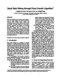
Applying Topology-Shape-Metric and FUZZY Genetic Algorithm for Automatic Planar Hierarchical and Orthogonal Graphs Nahla F.Omran

Sara F. Abd-el ghany

Department of mathematics Faculty of science, South Valley University Qena, Egypt

Qena, Egypt

Abstract—The graphs appear in many applications such as computer networks, data networks, and PERT networks, when the network includes a small number of devices, it can be drawn easily by hand, as the number of devices increases, drawing becomes a very difficult task. For this problem we will develop a new method for automatic graph drawing based on two steps, the first is applying the topology –shape –metric that is approaching to orthogonal drawings for the grid and the second step is applying the fuzzy genetic algorithm that is directed, in the topology –shape –metric the final drawing is achieved through three sequential steps: planarization, orthogonalization, and compaction. Each of these steps is responsible for the quality of the final drawing. Then the genetic algorithm applied at the planarization step of the topology-shape-metric to find the geometric position of each vertex to minimize bending in the graph. The developed technique generates a greater number of planar embedding by varying the order of edges’ insertion. This is achieved clearly in the Results given in the paper. Keywords—graph drawing; hierarchical graphs; topologyshape-metric; fuzzy genetic algorithms

I.

INTRODUCTION

The expanding use of computers into business, science and the home, making scientists tend to draw diagrams to understand computer software. Graph drawing is a visualization of objects and relations between those objects. The effectiveness of the visualization of a graph is dependent on how efficiently the associated diagram conveys information to the users. The Specific requirements in this application are: Initially we will apply the topology- shapemetric that is divided into three main steps. The first step is the planarization step in this step reduces the number of edge crossings as much as possible. The second step is the Orthogonalization: The goal of this step is to minimize the number of bends without changing the topology. The third step is the compaction in this step the goal is to minimize the drawing area. The problem of drawing graph was first studied in 1983 by M.R Garey, and D.S. Johnson [1] studied the problem of minimizing the number of edge-crossing. Then, in 1994, Di Battista [2] presented study to produce esthetically pleasing drawings of graphs based on main-cost-flow for both vertical and horizontal edge groups. Later, in 1999 Klau, Petra Mutzel [3] presented an approach based on a branch – and – cut algorithm which computes

optimally labeled orthogonal drawings for compaction and labeling problem. In 2001, Maurizio patrignani [4] presented study for the complexity of orthogonal compaction based on three problems consist of providing an orthogonal grid drawing, while minimizing the area , the total edge length, or the maximum edge length. In 2002 Markus Eiglsperger, Michael Kaufman [5] present a new compaction algorithm for orthogonal graph drawing with vertices of prescribed size. Finally, applied the fuzzy genetic algorithm at the planarization step of the TSM. The use of fuzzy logic based techniques for either improving genetic algorithm behavior and modeling genetic algorithm components, the results obtained have been called a Fuzzy genetic algorithm. A FGA may be defined as an ordering sequence of instruction in which some of the instructions or algorithm components may be designed with fuzzy logic- based tools. In 1960[6], the Genetic Algorithms were first described by John Holland and further developed by Holland and his students and colleagues at the University of Michigan in the 1960 and 1970.In 1997, J.Branke, F.Bucher, H.Schmeck [7] use genetic algorithm for undirected graphs. In 1999, D.K.Pratihar, K.Deb, A.Ghosh [8] uses a fuzzy logic and a fuzzy genetic algorithm for the problems with mobile robots. In 2001, I.G. Damousis, K.J. Satsio's, D.P. Labridis, P.S. Dokopoulos [9], combined fuzzy logic and genetic algorithm techniques—application to an electromagnetic field problem. In 2006, P.Kuntz, B.Pinaud, A.Ghosh [10] used a hybrid genetic algorithm to minimizing crossing in hierarchical graphs. In 2007, D.Vrajitoru [11] applied a hybrid genetic algorithm to solve graph drawing problems. In 2011, Bernadette M.M, Gustavo H.D, Frederico G. Guimar, Renato C. M, Petr Ya. E [12] using a fuzzy genetic algorithm for automatic orthogonal graph drawing. In this chapter we will use TSM to minimize the crossing in the graph and then apply the FGA in the second step of TSM to find the geometric position of each vertex to minimize the bends in the graph to produce a graph with good esthetic criteria. II.

THE TOPOLOGY – SHAPE – METRIC TECHNIQUE

The topology-shape-metric was widely discussed and improved in 1998 by I.G. Toll's, G. Di Battista, P. Eades, and R. Tamassia [13]. When applying the topology-shape-metric, the final drawing is produced by applying three consecutive steps: planarization, orthogonalization, and compaction.

81 | P a g e www.ijacsa.thesai.org


A. Planarization this step determine the topology of the graph , which test if the graph is planar or no. therefore, the goal of this step is to minimize the number of edge crossing as much as possible because the number of crossing affects the understanding of the graph. In 1998, I.G. Toll's, G. Di Battista, P. Eades, R. Tamassia [13] present algorithms that are used to build planar graph.

We will apply the planarization step on the graph in Figure2, we will get different planar graph by varying edge insertion to minimize edge crossing. 1

2

3

6

4

7

5

8

9

Fig. 2. Example of nonplanar hierarchical graph. 1

2

3

6

4

7

8

5

9

Fig. 1. Block diagram for the topology-shape-metric algorithm [14, 15]

Algorithm (Planarize). Input: graph G; Output: planarization G_ of G; 1) Compute a maximal planar subgraph S of the input graph G, and partition the edges into “planar” and “nonplanar”, as follows: a) Start with subgraph G_ consisting only of the vertices of G, but no edges; b) For each edge e of G, if the graph obtained by adding e to G_ is planar, then add e to G_ and classify e as “planar”, else reject e and classify it as “non planar”. 2) Construct a planar embedding of the planar subgraph G_, and the dual graph of S. 3) Add to G_ the non planar edges, one at a time, each time minimizing the number of crossings. This is done as follows for a non planar edge (u, v): a) Find a shortest (least number of edges) path in the dual graph of the current embedding G_ from the faces incident to u to the faces incident to v; b) Add the nonplanar edge and update G_ as well as its dual graph.

Fig. 3. Nonplanar hierarchical graph with one bend. 1

2

3

6

7

4

8

5

9

Fig. 4. Planar hierarchical graph with three bends.



The graph in Figure4 is planar but contains three bends, to solve this problem we will apply fuzzy genetic algorithm. B. Orthogonalization This step is performed to reshape the drawing to cancel the bends from the graph and the edge become straight line. We will use the Tamassia algorithm [14] computes an orthogonal shape of a planar graph with respect to an input embedding with a minimal number of bends the result of the orthogonalization on the Figure2 is shown in Figure5. Algorithm. ORTHOGONAL Input. A biconnected graph G. Output. An orthogonal drawing of G. 1) Compute a st-numbering of G 2) Produce a reduced graph G I and modify the stnumbering so that there are no gaps in the st sequence. 3) Run Form _pairs on the reduced graph G. 4) Place vertices vl and v2 in the same row, if v2 does not belong to a pair in which it shares a row with another vertex. If Vl and/or v2 have degree less than 4, then the placement of vl and v2 might require one or two rows. 5) REPEAT a) Consider the next vertex vi according to Unmarked. The st-numbering of G. b) If v has already been placed, then go to Step 6. c) If vertex vi is unassigned, then place v, i in a new row. Connect vi with each vertex vj (j < i) such that (vj, vi) is a directed edge of G. Add as many uncompleted edges as required, depending on vi's out degree. d) If vertex vi is assigned to a pair, then place vi together with the other vertex in the same pair following the placement rules described above for the specific type of pair. 6) UNTIL the only remaining vertex is vn, 7) Insert vn, in a new row. If vn, is of degree 4, then there is an incoming edge that enters vn, from the top and bends twice. This edge is chosen to be the one that connects to vn, _l. 8) Restore the degree 2 vertices of G that were absorbed in Step 2. 9) End.

C. Compaction In this section we will minimize the area of the given orthogonal drawing. The result of this step is shown in Figure6. Algorithm .planar graph compaction. Input. √n x. √n bitmap planar graph layout. Output. √n x. √n bitmap planar graph layout compacted one point to the east. 1) identify all points on layout that may possible move to the east. Mark these points to be movable. 2) umark movable points that can cause connectivity violation to be stationary. 3) repeat step 2 until no further points is unmarked. 4) compact movable points to one point to the east maintaining connectivity.

Fig. 6. The result of compaction Figure5

III.

PROPOSED FUZZY GENETIC ALGORITHM

We will solve the problem of bending in the graphs by using the FGA to find the geometric position of each vertex. We will applying the FGA at the planarization step to obtain a lot of planar graphs then submit this to orthogonalization and compaction step .The aesthetic criteria takes into consideration: 1) The number of crossings FX in the graph. 2) The number of bends fB in the graph. 3) The total sum of the edges’ length fL. By minimizing all of them we will obtain the optimal graph. The fitness function ф(st,i) = α1fX + α2fB + α3fL where i ∈ [0, 1] We develop the diagram of TSM by adding FGA [15]. Algorithm (TSM-Fuzzy-GA). Input: graph G; Output: an optimized planar drawing; 1) Generation of the initial population: N = number of individuals;

Fig. 5. Orthogonal representation of Figure2

a) Generate at random the ordering of edge’s insertion from G (represented by an integer permutation);



2) Fitness computation: i = 0; While (i < N) do

1

a) Submit solution si to the planarization step to obtain a planar embedding (Γ i) and the number of crossings FX (si); b) Submit the planar embedding (Γ i) to the orthogonalization step to obtain the orthogonal representation H, and the number of bends fB (si); c) Submit the orthogonal representation H to the compaction step to obtain the final drawing and the total sum of the edges length fL (si); d) Calculate the value of the fuzzy membership's µFX, µFB, and µFL; e) Calculate the fuzzy-max-min aggregation µD; f) i = i +1; 3) Record the best individual according to the fitness function; 4) Application of the genetic operators for generating the new population. Each crossover operator (PMX or OX) for producing each offspring is selected with equal probability (0.50). The mutation operator to be used (scramble, swap, insert, and invert) for each offspring is also selected at random with equal chance (0.25); 5) Application of generational survival selection; 6) Go to step 2 until the stop criterion is met; The results of applying FGA on the Figure2. First step: in Figure7 we replaced v2 by v3 to cancel the bend between v2 and v7. Second step: in Figure8 we replaced v8 by v9 to cancel the bend between v5 and v8. 1

3

2

6

7

4

8

5

9

3

2

6

7

4

9

5

8

Fig. 8. Best planar graph produced from applying FGA

IV.

A GENETIC OPERATOR

in this paper we attempt to solve the problem of bends in the graph by using FGA, the operator used in genetic algorithms to maintain genetic diversity, known as mutation and to combine existing solutions into others, crossover. The main difference between them is that the mutation operators operate on one chromosome, that is, they are unary, while the crossover operators are binary operators .Genetic variation is a necessity for the process of evolution. Genetic operators used in genetic algorithms are analogous to those in the natural world: survival of the fittest, or selection, reproduction (crossover, also called recombination), and mutation. A. Selection The Selection operator decides which of the individuals in the population will go into the next generation. This is decided by the fitness value of an individual as calculated by the Fuzzy Fitness Function. At this point the assumption is that a fitness value pertaining to each individual is available. B. Crossover Crossover is the most widely used recombination operator. Uniform 1-point crossover has been used. In general, 1-point crossover selects a random cut point and combines the first portion of one parent with the second portion of the other and vice versa to produce two offspring. The individual here consists of an array of cluster numbers. Hence, the main issue in recombination is the renumbering of clusters in the resulting offspring.

Fig. 7. Planar graph result from applying FGA



made a single-point cluster to which zero fitness value is assigned. d) Mutation Rule 4: if none of the above conditions apply, then the border is left undisturbed.

Fig. 9. A Visualization of Crossover

C. Mutation Mutation is needed to counteract the loss of some potentially useful genetic material during selection and crossover. In an artificial chromosome, this is affected by an Occasional random alteration of the value of a string position. In a binary implementation, a bit value is toggled. In an integer or floating point implementation, a value is changed within an allowed range. This definition cannot be directly applied to the present scenario .A mutation operator that works at the boundaries of clusters has been worked out. For this, the pair-wise fitness between two consecutive data points is found for the whole data set. This has been calculated using the Fuzzy Fitness Function. 1) In each, select randomly, points in the range (1, mi) where mi is the number of clusters in the ith individual. The number of clusters to be selected is equal to n mutation as worked out in the previous paragraph. Mutation is applied on the left as well as on the right border of each selected cluster which amounts to 2*n mutation borders. 2) for a border point Two cut-off values (in %) are to be fixed, one below which the pair-wise fitness will be classified as insignificant (lower value (lval)) and the other above which the pair-wise fitness will be significant (high value) hval). The actual values will be implementation dependent.

Fig. 10. A Visualization of Mutation

V.

RESULTS

In this paper, we tested many values for the number of vertices v in the graph, to generate an optimal graph by following the procedure shown in the diagram [16]: 1) We generated graphs by varying the number of vertices V, from 10 to 600 vertices. 2) For each graph in the test set, when we applying the TSM on the graph in Figure2, at the planarization step the final graph contain three bends shown in Figure5, but when we applying FGA at the planarization step on the Figure2, the final graph contains one bend shown in Figure7. Table 1 shows the results obtained with the classical topology shape-metric approach. Table 2 presents the results obtained by the fuzzy genetic algorithm. TABLE I.

a) Mutation Rule1: if it's pair-wise fitness with the data point in the neighboring cluster is greater than hval and its pair-wise fitness with the neighboring data point within the same cluster is less than lval, and then reallocates the data item to the neighboring cluster. b) Mutation Rule 2: if it's pair-wise fitness with the data point in the neighboring cluster is greater than hval and also its pair-wise fitness with the neighboring data point within the same cluster is greater than hval, then the two clusters can be merged. c) Mutation Rule 3: if it's pair-wise fitness with the data point in the neighboring cluster is less than lval and its pairwise fitness with the neighboring data point within the same cluster is also less than lval, then the border point can be

RESULTS OBTAINED BY THE CLASSICAL APPROACH TSM

F 41 87 148 232 441 1398 2126 2757 4769 5969 9055 9500 10000 10100

fl 16 38 64 92 132 328 632 781 854 1144 2748 2800 3000 3200

fB 3 2 5 6 19 49 59 75 172 197 173 198 200 195

fx 0 1 1 6 24 119 137 194 509 618 608 620 630 616

v 10 20 30 40 50 100 150 180 200 250 500 520 550 600


(IJACSA) International Journal of Advanced Computer Science and Applications, Vol. 6, No. 5, 2015 TABLE II.

V-N 10-30

20-30

30-30

40-30

50-30

100-30

150-30

180-30

200-30

250-30

500-30

520-30

550-30

Fig. 11. Block diagram for the TSM-Fuzzy-GA algorithm

600-30

RESULTS OBTAINED BY THE FUZZY GENETIC ALGORITHM

Fuzzy genetic algorithm stats fx fl Best Average StdDev Best Average StdDev Best Average StdDev Best Average StdDev Best Average StdDev Best Average StdDev Best Average StdDev Best Average StdDev Best Average StdDev Best Average StdDev Best Average StdDev Best Average StdDev Best Average StdDev

0 0 0.00 1 1 0.00 1 1 0.00 5 5 0.52 12 14 1.69 62 70 7.89 86 89 5.56 95 110 10.27 334 342 18.57 427 429 12.77 319 321 2.67 310 303 1.90 367 332 20.23

14 14 0.52 29 30 0.95 48 50 1.69 71 76 4.37 95 100 7.66 250 264 8.29 393 403 25.33 531 536 35.14 687 688 34.21 910 999 77.81 1351 1356 6.86 1387 1493 6.92 1400 1525 50.72

Best Average StdDev

358 290 2.29

1520 1526 7.67

Test cases fB µD 3 3 0.00 1 1 0.00 5 5 0.00 5 6 0.71 10 12 1.96 31 36 3.30 36 38 3.08 51 52 2.17 120 130 5.91 145 152 4.47 103 108 6.98 95 87 5.00 163 145 7.10 150 110 7.80

1.000 0.800 0.26 1.000 0.675 0.24 1.000 0.714 0.25 0.857 0.433 0.26 0.769 0.446 0.23 0.917 0.330 0.31 1.000 0.237 0.29 0.696 0.321 0.26 0.698 0.198 0.26 0.848 0.279 0.35 1.000 0.697 0.41 1.100 0.699 0.50 0.900 0.770 0.40 1.900 0.800 0.56



VI.

CONCLUSIONS

ACKNOWLEDGMENT

In this paper, we present a new method for automatic orthogonal graph drawing by using fuzzy genetic algorithm at the planarization step of the topology-shape-metric to find the geometric position of each vertex to obtain optimal graphs without crossing and bends.

I cannot express my feelings to my family who supported me all over through my way and backed me up during my studies wishing me good luck throughout the preparation of this thesis. [1] [2]

[3]

[4] [5]

[6]

[7]

[8]

[9]

[10]

[11]

[12]

[13] [14]

[15] Fig. 12. V = 100: (a) drawing obtained with topology-shape-metric (b) drawing obtained with the fuzzy genetic algorithm

[16]

REFERENCES M.R. Garey, D.S. Johnson, Crossing number is NP-complete, SIAM Journal on Algebraic and Discrete Methods 4 (1983), pp.314-316. G. Di Battista, P. Eades, R. Tamassia, I. Toll's, Annotated bibliography on graph drawing algorithms, Computational Geometry: Theory and Applications 4 (1994), pp. 240–282. G.W. Klau, P. Mutzel, Optimal compaction of orthogonal grid drawings, in: 7th International Integer Programming and Combinatorial Optimization (IPCO) Conference, volume 1610 of Lecture Notes in Computer Science, Springer, 1999. M. Patrignani, on the complexity of orthogonal compaction, Computational Geometry 19 (2001), pp. 50 – 60. M. Eiglsperger, M. Kaufmann, Fast compaction for orthogonal drawings with vertices of prescribed size, in: 9th International Symposium on Graph Drawing (GD 2001), volume 2265 of Lecture Notes in Computer Science, Springer, 2001. Holland, J. H. (1992). Genetic algorithms. Scientific American, July, 114–116. Forrest, S. (1993). Genetic algorithms: Principles of natural selection applied to computation. Science, 261, 872-878. J. Branke, F. Bucher, H. Schmeck, Using genetic algorithms for drawing undirected graphs, in: The Third Nordic Workshop on Genetic Algorithms and their Applications, 1997, pp. 200–205. D.K. Pratihar, K. Deb, A. Ghosh, Fuzzy-genetic algorithms and timeoptimal obstacle-free path generation for mobile robots, Engineering Optimization 1 (1999),pp. 117–130. P. Kuntz, B. Pinaud, R. Lehn, Minimizing crossings in hierarchical digraphs with a hybridized genetic algorithm, Journal of Heuristics 12 (2006) 30–36. I.G. Damousis, K.J. Satsios, D.P. Labridis and P.S. Dokopoulos," Combined fuzzy logic and genetic algorithm techniques—application to an electromagnetic field problem"Elsevier,2001, pp.371-385. D. Vrajitoru, Hybrid multiobjective optimization genetic algorithms for graph drawing, in: Proceedings of the Genetic and Evolutionary Computation Conference (GECCO 07), ACM Press, 2007. Bernadette M.M. Neta Gustavo H.D. Arajo,ْ Frederico G. Guimaraes, Renato C. Mesquita, Petr Ya. Ekelc '' A fuzzy genetic algorithm for automatic orthogonal graph drawing'' journal of SciVerse Science Direct, 2011, pp, 1379-1380. I.G. Toll's, G. Di Battista, P. Eades, R. Tamassia, and Graph Drawing: Algorithms for the Visualization Of Graphs, Prentice Hall, 1998. R. Tamassia, New layout techniques for entity-relationship diagrams, in: Proceedings of the Fourth International Conference on EntityRelationship Approach, IEEE Computer Society, Washington, DC, USA, 1985, pp. 304–311. T. Lengauer, Combinatorial algorithms for integrated circuit layout, John Wiley & Sons Inc., New York, NY, USA, 1990 Bernadette M.M. Neta Gustavo H.D. Arajo, Frederico G. Guimaraes, Renato C. Mesquita, Petr Ya. Ekelc '' A fuzzy genetic algorithm for automatic orthogonal graph drawing'' journal of Sci Verse Science Direct, 2011, p, 1385.


Applying Topology-Shape-Metric and FUZZY Genetic Algorithm for ...

Applying Topology-Shape-Metric and FUZZY Genetic Algorithm for ...

Suggest Documents