Industrial Engineering & Management Systems Vol 14, No 1, March 2015, pp.1-10 ISSN 1598-7248│EISSN 2234-6473│
http://dx.doi.org/10.7232/iems.2015.14.1.001 © 2015 KIIE
Applying Genetic Algorithm for Can-Order Policies in the Joint Replenishment Problem Keisuke Nagasawa*, Takashi Irohara Department of Information and Communication Sciences, Sophia University, Tokyo, Japan Yosuke Matoba, Shuling Liu Fairway Solutions Inc., Tokyo, Japan (Received: January 5, 2014 / Revised: October 6, 2014; February 17, 2015 / Accepted: March 9, 2015) ABSTRACT In this paper, we consider multi-item inventory management. When managing a multi-item inventory, we coordinate replenishment orders of items supplied by the same supplier. The associated problem is called the joint replenishment problem (JRP). One often-used approach to the JRP is to apply a can-order policy. Under a can-order policy, some items are re-ordered when their inventory level drops to or below their re-order level, and any other item with an inventory level at or below its can-order level can be included in this order. In the present paper, we propose a method for finding the optimal parameter of a can-order policy, the can-order level, for each item in a lost-sales model. The main objectives in our model are minimizing the number of ordering, inventory, and shortage (i.e., lost-sales) respectively, compared with the conventional JRP, in which the objective is to minimize total cost. In order to solve this multi-objective optimization problem, we apply a genetic algorithm. In a numerical experiment using actual shipment data, we simulate the proposed model and compare the results with those of other methods. Keywords: Inventory Modeling and Management, Logistics and Supply Chain Management(L/SCM), Supply Chain Management(SCM), Evolutionary Algorithms, Warehouse Operation and Management * Corresponding Author, E-mail:
[email protected]
1. INTRODUCTION Effective inventory management has played an important role in the success of supply chain management. It is important in inventory management to decide when and how much ordering of item. Usually, effective inventory management is expected to lead to reduced amounts of inventory and shortage by proper ordering policies for each item. One well-known inventory model is the single warehouse multi-retailer (SWMR) problem (e.g. Chan et al., 2002). In the general SWMR problem, retailers know external demand of items over a finite planning horizon. Items are shipped from the suppliers to the warehouse and distributed from the warehouse to the retailers. The goal of this problem is to find an optimal replenishment
timing and quantity to minimize the total transportation cost or inventory costs in the system. For multi-item inventory control, the joint replenishment problem (JRP) coordinates the ordering quantity of several items in a warehouse. For example, let us consider a warehouse with items supplied by only one supplier. When the inventory manager orders many items from the same supplier, the ordering cost charged depends on the number of orders and the number of different items ordered. Therefore, the ordering quantities of different items cannot be decided individually. The typical assumptions of the JRP are similar to those in the conventional economic ordering quantity model. These include (i) the demand is deterministic and constant, (ii) shortages are not allowed, (iii) there are no quantity discounts, and (iv) the inventory cost is linear.
Nagasawa, Irohara, Matoba, and Liu: Industrial Engineering & Management Systems
Vol 14, No 1, March 2015, pp.1-10, © 2015 KIIE
Goyal (1974) developed an algorithm to find the optimal solution under the classical JRP. Then Silver (1976) developed an efficient heuristic algorithm for solving this problem, which Kaspi and Rosenblatt (1991) improved. Reviews of the literature of JRP can be found in Goyal and Satir (1989) and Khouja and Goyal (2008). Recently, Amaya et al. (2013) proposed a new heuristic algorithm for solving the JRP under deterministic demand and resource constraints. Yang et al. (2012) applied a genetic algorithm (GA) to the problem in which there are known multi-item demands, multiple retailers, a finite planning horizon, and cost functions including discounting, and then found the optimal total cost. Wang et al. (2012b) proposed a new differential evolution algorithm for joint replenishment. Wang et al. (2012a) proposed an efficient hybrid differential evolution algorithm for joint replenishment with delivery, as a traveling sales man problem. A can-order policy is one type of inventory management policy applied to the JRP. Can-order policies were originally suggested by Balintfy (1964), after which van Eijs (1994) showed that can-order policies are at least as good as other coordinated replenishment policies. A can-order policy is represented by a set of three parameters: (si, ci, Si), or simply (s, c, S). When the inventory level of item i drops to or below si, called the reorder level, an order is placed to bring the inventory level up to Si, called the order-up-to level. For any other items, j, whose inventory levels are less than their respective can-order levels, cj, orders will also be placed so that inventory levels of items j are raised to Sj. Federgruen et al. (1984) modeled a can-order policy as a semi-Markov decision problem with compound Poisson demands and positive lead-times. They showed that a can-order policy is considerably better than uncoordinated policies, often providing as much as a 20% savings. Most previous research on can-order policies focuses on how to derive the optimal (s, c, S) values based on the algorithm. This line of research assumes that each levels of can-order policy, s, c and S, cannot fix to some value or that the correlated demand probabilities between any two items are already known (see, for example, Liu and Yuan (2000)). However, this assumption introduces difficulties which make a can-order policy hard to apply to large problems. Furthermore, the Federgruen et al. (1984) decomposition approach may introduce substantial errors (Atkins and Iyogun (1988), Pantumsinchai (1992), Dellaert and Poel (1996), Melchiors (2002) and Johansen and Melchiors (2003)). The difficulty is that knowing how to define the demand relationships between each pair of items is often not enough in practice: a demand correlation among each triplet of items should be defined in advance. Tsai et al. (2009) proposed an association clustering algorithm to evaluate the correlated demands among multiple items. Their algorithm utilizes the “support” concept to measure the demand similarity among items. Based on these
2
measurements, a clustering method is developed to group items with close demand and a can-order policy is applied to the clustering result. Zhao et al. (2011) proposed a new clustering algorithm for can-order policies. A good summary of other applications of can-order policies can be found in Kayis et al. (2008). Most previous research on JRP or can-order policies focuses on how to derive the optimal ordering quantity or (s, c, S) values based on the algorithm. The researches have assumption that the ordering quantities or ordering levels, (s, c, S) values of different items cannot be decided individually. This line of research assumes that each levels of can-order policy, s, c and S, cannot fix to some value. But, in actual inventory management, there are constraints of service level, related to s, or capacity limitation of shelf for each item, related to S. In our research, because the can-order levels of many items should be set under the situation where reorder levels and order-up-to levels of each items should be fixed. Thus, we optimize the can-order level of each item by heuristic method. In this study, we compare the ordering penalty, the inventory penalty, and the shortage penalty. Therefore, we define this problem as a multiobjective optimization problem. Therefore, we optimize can-order level of each item by genetic algorithm, which is well applied to multi-objective optimization problem. In our research, we determine proper can-order level of each items, and minimizes each objective value. Even if the problem is single-objective mathematical formulation, the model is NP-hard. The mathematical model can solve a small size problem in few items and short planning period. Since optimizing the size of our problem took too long time, we proposed GA for deciding can-order level. And, because GA is well used for similar problem (Khouja et al. (2000) used GA for classical JRP, Moon and Cha (2006) confirm some extent of effectiveness of GA for constrained JRP, or Yang et al. (2012) used GA for SWMR), and GA is well used for multi objective optimization problem. Thus, this research also proposed and applied GA for deciding can-order level. Even if we can calculate total cost, where the sum of the three costs can be calculated, our proposed method can use by changing the calculation method of fitness value related to total cost. The remainder of this paper is organized as follows. The mathematical formulation for the deterministic demand model is presented in Section 2. In Section 3, we propose a GA for obtaining can-order levels for the stochastic demand problem when the re-order level and order-up-to level are decided separately for each item. The computational results are described in Section 4. Finally, conclusions are presented in Section 5.
2. PROBLEM FORMULATION Herein, we assume the existence of stable shipping data comprising the shipping date and order volumes of
Applying Genetic Algorithm for Can-Order Policies in the Joint Replenishment Problem Vol 14, No 1, March 2015, pp.1-10, © 2015 KIIE
items. For each item, i, the ordering policy is taken as (si, ci, Si), where the re-order level, si, and order-up-to level, Si, are parameters, and we decide the can-order level, ci. The features of our research are shown below and we formulate the problem as follows. We consider a multiitem inventory management problem in which a warehouse sells multiple items with no quantity discounts. Items can be kept in storage with a holding penalty and do not deteriorate. When demands cannot be fulfilled, items on hand are shipped and the shortage demand induces a lost-sales penalty. In this problem, ordering penalty, inventory penalty, and shortage penalty are the objective functions. When the demands are deterministic and replenishment from a supplier is periodic in a finite planning period, the multi-item inventory problem with a canorder policy can be formulated as follows: minimize f1 = minimize f 2 = minimize f 3 =
∑u y t
∀t ∈T
(1)
t
∑ ∑ po
(2)
∑ ∑hl
(3)
∀i∈I ∀t ∈T
∀i∈I ∀t ∈T
i i t t
i i t t
lti−1 + xti − lti + oti = d ti ,
∀i ∈ I , ∀t ∈ T ,
x ≤ Myt l t −1 − d t + o t + Mr t ≥ s i
i
i
i
∀i ∈ I , ∀t ∈ T , ∀i ∈ I , ∀t ∈ T ,
(15)
∀i ∈ I , ∀t ∈ T ,
(16)
∀i ∈ I , ∀t ∈ T ,
i
l t −1 − d t + o t − M(1 − r t ) ≤ s i
(4) (5) (6) (7) (8) (9) (10) (11) (12) (13) (14)
∀i ∈ I , ∀t ∈ T ,
i t
i
i
∀i ∈ I , ∀t ∈ T ,
i
S i ≤ l i t −1 − d i t + oi t + x i t + M(1 − r i t )
∀i ∈ I , ∀t ∈ T ,
S ≥ l t −1 − d t + o t + x t − M(1 − r t )
∀i ∈ I , ∀t ∈ T ,
i
i
S ≥c i
i
i
i
i
∀i ∈ I ,
i
ci ≥ si
∀i ∈ I ,
l i t −1 − d i t + oi t + Mk i t ≥ c i l t −1 − d t + o t − M(1 − k t ) ≤ c i
i
i
i
∀i ∈ I , ∀t ∈ T , ∀i ∈ I , ∀t ∈ T ,
i
qit ≤ k it qit ≤ qit ≥
∑r
∀i∈I
i t
1 ∑ r i t − (1 − k i t ) | I | −1 ∀i∈I
S i ≤ l i t −1 − d i t + oi t + x i t + M(1 − q i t ) S ≥ l t −1 − d t + o t + x t − M(1 − q t ) i
i
i
i
i
x i t ≤ M(r i t + q i t ) oi t ≤ d i t
i
∀i ∈ I , ∀t ∈ T ,
(17) ∀i ∈ I , ∀t ∈ T , (18) ∀i ∈ I , ∀t ∈ T , (19) ∀i ∈ I , ∀t ∈ T , (20)
yt , r i t , k i t , q i t ∈ {0, 1},
∀i ∈ I , ∀t ∈ T
l , x , o , c ∈ Z+
∀i ∈ I , ∀t ∈ T
i t
i t
i t
lti:inventory level of item i on the t th day xti : the ordering quantity of item i on the t th day rti : if lti drop below s i , then rti = 1; otherwise, rti = 0
kti : if lti drop below c i , then kti = 1; otherwise, kti = 0 qti : if lti drop below c i ( ⇔ kti = 1) and
at least one item is ordered at t th day( ⇔ max( rti ) = 1), ∀i∈I
then qti = 1; otherwise, qti = 0
Parameters ut : fixed ordering penalty on the t th day
pti : lost sales penalty of item i on the t th day hti : penalty of holding one unit item i on the t th day d ti : demand of item i on the t th day S i : the order up to level of item i
s i : the reorder level of item i M : big-M I : the set of items T : the set of days
subject to
i
3
i
Decision variables yt : if order is placed in t th day, then yt = 1; otherwise yt = 0 c i : the can order level of item i
oti : the lost sales quantity of item i on the t th day
The first objective function (Eq. (1)) considers the fixed ordering penalty within the planning period. The second objective function (Eq. (2)) considers the shortage penalty within the planning period. The third objective function (Eq. (3)) considers the inventory penalty within the planning period. Eq. (4) is the inventory balancing equation for all items. Eq. (5) is a constraint on ordering when there is ordering of items within each planning period. By constraints (6) and (7), if the inventory level drops to or below the re-order level, an order will be placed. Furthermore, by constraints (8) and (9), when the inventory level drops to or below the re-order level, the order quantity is set as the difference between the order-up-to level and the inventory level. Constraint (10) represents that each can-order level is no more than the order-up-to level. Constraint (11) represents that each re-order level is no more than the can-order level. Constraints (12) and (13) identify whether the inventory level of an item has dropped to or below its can-order level. By constraints (14), (15), and (16), when the inventory level of at least one item has dropped to or below its reorder level, an order is placed that includes items for which the inventory level has dropped to or below the can-order level. By constraints (17) and (18), the items for which the inventory level has dropped to or below the can-order level will be ordered in the quantity equal to the difference between the order-up-to level and the inventory level. Constraint (19) represents that items for which the inventory level has dropped to or below the can-order or the re-order level can be ordered. Constraint (20) represents that the shortage amount of each item is no more than the demand of the corresponding period.
Nagasawa, Irohara, Matoba, and Liu: Industrial Engineering & Management Systems
Vol 14, No 1, March 2015, pp.1-10, © 2015 KIIE
The problem is multi-objective optimization problem. Therefore we propose real value genetic algorithm for deciding can-order level of each item. If fixed ordering cost, holding cost and shortage cost are assessed exactly, and if each function are same units, we can make single objective optimization. But, the mathematical optimization problem model is still known as NP-hard.
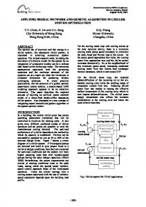
3. IMPLEMENTATION OF GENETIC ALGORITHM (GA) In this study, the mathematical formulation at previous chapter could not be solved by mathematical optimization solver, because it is multi-objective optimization model. We apply a can-order policy for an item set. For the model, a GA was applied in order to obtain a better solution than deciding the ordering quantity of each item separately, according to the number of order, the amount of shortage, or the amount of storage. In addition, because we used simulation for evaluating each level of ordering policy, we can set each level of ordering policy for the situation where demands are stochastic or where inventory manager does not know future demand. In order to solve the multi-item inventory problem with a can-order policy, we used a GA approach. A GA is an adaptive heuristic search algorithm based on the evolutionary concept of natural selection. The basic concept of a GA is to simulate processes in a natural system that are necessary for evolution, specifically the processes that follow the principles of survival of the fittest first laid down by Charles Darwin. As such, these processes represent an intelligent exploitation of a random search within a defined search space for the purpose of resolving a problem. GAs are typically used to solve combinatorial problems that cannot be handled by exhaustive, multi-objective, or exact methods, due to their prohibitive complexity. Start Initialization Calculate fitness function Genetic operation
Selection
4
The basic procedure of the GA approach is to code the decision variables of the problem as a finite-length array (referred to as a chromosome) and calculate the objective value (fitness) of each chromosome. Based on the fitness, the probability of survival for each chromosome is calculated. The surviving chromosomes then reproduce and form the chromosomes of the next generation through crossover and mutation processes. Figure 1 shows the outline of a GA. 3.1 Chromosome Representation A chromosome is a set of genes related to the solution of the problem. A critical issue when applying GAs to an optimization problem is the selection of a suitable encoding scheme for transforming feasible solutions into genetic representations and vice versa. In the present paper, we assume that the order-upto level, Si, and the re-order level, si, of each item are fixed value and we decide the separate can-order level. In this study, as shown in Table 1, if we define the number of items as n and define the number of members of the set of binary string genes for each item as m, the can-order level of all items can be represented by an nmlength chromosome. The can-order level of each item is determined from the corresponding m-length string of binary genes. The values of each gene are taken as 0 or 1, and each gene is referred to as a bit. In some GAs, encoding and decoding are carried out using binary strings. Traditional binary coding for function optimization is known to have a weakness due to the large change of a real parameter value arising from changing a single bit in the binary string of the parameter. For example, the binary strings 01111111 and 11111111, which differ in only one bit, correspond to the decimal numbers 63 and 127, respectively. “Gray code” (Gray, 1953) is alternative method of encoding parameters in terms of bits. Gray code has the property that an increase by one step in the value of a design variable corresponds to the change of a single bit in the binary string of the design variable. Andre et al. (2001) compared binary coding and Gray coding in terms of GAs using two-point crossover and concluded that Gray coding helped to improve the speed relative to binary coding. The conversion from Gray coding to bik nary coding is given by bk = ∑ i =1 g i ( mod 2 ). We decode the m-length gene section of each item to a can-order level as a Gray code.
Crossover
Table 1. Example chromosome of the genetic representation scheme
Mutation Termination?
No
Yes End
Figure 1. Outline of a genetic algorithm.
Item : i 1 2 n Index of gene 1 … m m+1 … 2m (n-1)m+1 … nm … 1 Gene 0 … 1 1 … 0 … 0 Can-order 7 15 5 level: ci
Applying Genetic Algorithm for Can-Order Policies in the Joint Replenishment Problem Vol 14, No 1, March 2015, pp.1-10, © 2015 KIIE
3.2 Initial Population During the initialization process, a predefined number of chromosomes are randomly generated to represent the can-order levels for all items. In this initialization phase, we also create special chromosome in which the can-order levels of each item correspond to their reorder levels by setting all of genes in this chromosome to zero, the chromosomes represent only using predefined order-up-to level and re-order level and not using can-order level. 3.3 Fitness Function A fitness function is a particular type of objective function that prescribes the optimality of a chromosome. Optimal chromosomes, or at least chromosomes with near-optimal values, are allowed to breed and mix their datasets following one of a number of techniques to produce a new generation with improved characteristics. In this study, the fitness function is defined in terms of the original objective functions. The fitness function of the chromosome, f (chromosome), is represented as follows: f ( chromosome ) =
f e ( chromosome ) − f e min 1 3 ⎛ ⎜⎜1 − ∑ 3 e =1 ⎝ f e max − f e min
⎞ ⎟⎟, ⎠
where fe (chromosome), e = 1, 2, 3, denotes the objective values defined by Eq. (1) through (3), respectively. These values are the results of the simulation when the chromosome is applied with the ordering policy. Here, femax is the maximum value in the current generation of objective function e calculated by the simulation results. Similarly, femin is the minimum value in the current generation. We calculate the fitness values at each generation and use them to improve the pool of potential solutions in the selection step. 3.4 Genetic Operations
dom selection. In this study, we use the roulette wheel selection method, in which the probability of being selected is directly proportional to the fitness of the chromosome. 3.4.2 Crossover The crossover operator roughly mimics biological recombination between two single-chromosome organisms. In the present study, we use a two-point crossover method. The crossover operation is illustrated in Figure 2. First, we select two parent chromosomes, indicated in the figure by red dashed lines ( ) and blue double lines ( ). In two-point crossover, subsequence of genes are randomly selected and exchanged relative to the parents to create two children (in the figure, the source parent of genes in a child is indicated by the same color/ line designations as those of the parents). The crossover points at which the chromosome is broken are randomly selected. If there is at least one crossover, child 1 and child 2 are created and replace the parents in the new population. However, with some probability, no crossover occurs and the parents are copied unchanged into the new population. The probability of at least one crossover occurring for a parent chromosome pair is usually set between 40 and 90%. 3.4.3 Mutation The mutation operator is used to maintain genetic diversity from one generation of a population of chromosomes to the next. Mutation should allow the algorithm to avoid local optima by preventing the population of chromosomes from becoming too similar to each other. The mutation operator is applied to each child solution resulting from the crossover operation and is usually defined as a change in the values of genes in a chromosome. In this study, as shown in Figure 3, the mutation operator changes one randomly selected gene, indicated by the red dashed line ( ). Mutation can occur on any chromosome with some small probability, usually set between 0.0001 and 0.1.
Once initialization and fitness calculation have been performed, the genetic operations, which include selection, crossover, and mutation, are carried out. Along with new fitness calculations, these operations are repeated until the termination conditions are satisfied. At the end of each round of genetic operations, a new generation of chromosomes is obtained from the processes described below for the next iteration, and it is hoped this process will eventually yield an optimal individual. 3.4.1 Selection The selection operator selects chromosomes in the population for producing the next generation. Well-fitting chromosomes are likely to be selected for the next generation. There are several selection methods, such as roulette wheel selection, tournament selection, and ran-
5
Figure 2. Basic procedure of the two-point crossover operation.
Nagasawa, Irohara, Matoba, and Liu: Industrial Engineering & Management Systems
Vol 14, No 1, March 2015, pp.1-10, © 2015 KIIE
6
well Pareto solutions. This method is called “adaptiveweight GA.” 4.3 Experimental Results
In this study, we use an (s, c, S) policy with fixed s and S and optimize the can-order level, c, of each item by GA. The can-order level of each items are represented by the bit strings, as shown in Table 1. We apply the GA for actual shipping data. We decode each gene and obtain can-order level of each item. By the canorder level and fixed s and S, we simulate the can-order policy and evaluate the combination of can-order levels of each item. The combination of can-order levels of each item is chromosome in GA. The fitness value of chromosome is from the simulation results. 4.1 Data Set In the numerical and simulation experiments, we used the actual data for the shipments of a distribution company for a one-year period. This distribution center orders items to several suppliers. In addition, the distribution center ordered 200 items to one specific supplier. We applied the proposed method and determine canorder level of those 200 items jointly. We simulated (s, c, S) policies to the shipping data and set the parameters as described below. The lead time, i.e., the time from when the items were ordered to when the items were delivered, was set to two days. Reorder level, si, of each item was set to the mean two-day demand over the year plus 95% safety stock for two days. The order-up-to level, Si, of each item was set to the mean 28-day demand over the year. The GA parameters in experimental results were set as follows. The probability of crossover occurring is 90%; the probability for mutation is 0.04%; the maximum number of generations is 5000; the number of chromosomes in each generation is 1000. Roulette selection was used at each generation as the selection operation. 4.2 Evaluation Criteria
2500 2000 Shortage
4. EXPERIMENT AND RESULTS
(s, S) Initial generation 5000th generation
1500
e rtag o h S
1000 500 0 20000
25000 30000 Inventory
35000
Figure 4. Pareto solutions of inventory vs. shortage. 350 300 250 Ordering
Figure 3. Basic procedure of the mutation operation.
The simulation results for the proposed model are shown in Figures 4, 5, and 6, which show the Pareto solutions for inventory vs. shortage, inventory vs. ordering, and shortage vs. ordering, respectively. In Figures 4, 5, and 6, the orange closed circles are the results of applying an (s, S) policy, which is an (s, c, S) policy with the can-order level, c, set to the same value as the reorder level, s. Blue triangles denote results from using the initial can-order level, which was decoded as a Gray code from a randomly generated chromosome taken from the initial generation. Red crosses denote the results of Pareto solutions at the chromosomes of the 5000th generations in the GA. As shown in Figure 4, in terms of shortage, the (s, S) policy is inferior to using a can-order policy by result of chromosome from the 5000th generation in the GA. Because the can-order levels were set separately for each item, the on-hand levels of inventory are high and prevent shortage. In addition, the increases in the inventory levels are relatively small.
(s, S) Initial generation 5000th generation
200 150 rdeing O
In this study, a higher fitness value represents and makes Pareto solution. Each of the three objective values of ordering penalty, inventory holding penalty and shortage penalty are evaluated from a simulation of the actual data. And, based on those three objective values, fitness values of each chromosome are calculated. By improving the fitness value in GA, the chromosomes, which represents the can-order policy for each item, become
100 50 0 20000
25000 30000 Inventory
35000
Figure 5. Pareto solutions of inventory vs. ordering.
Applying Genetic Algorithm for Can-Order Policies in the Joint Replenishment Problem Vol 14, No 1, March 2015, pp.1-10, © 2015 KIIE
(s, S) Initial generation 5000th generation
Shortage
2000 1500 1000 500 0 20000
25000 30000 Inventory
35000
Figure 6. Pareto solutions of ordering vs. shortage. As shown in Figure 5, the inventory level of the (s, S) policy is low, since there are a large number of orders. The number of orders was reduced by using the canorder level by the GA for 5000th generations. This is because items, which are ordered separately under the (s, S) policy, are ordered jointly when applying the can-order policy. However, the inventory levels were higher under the can-order policy with the GA. As shown in Figure 6, when a (s, S) policy is used, the number of orderings is high and the shortage is large. The proposed method succeeded in reducing the number of orderings, and the amount of shortage. Since there were high inventory levels, the number of orderings and the amount of shortage decreased under the can-order policy because of increased opportunities for joint ordering. Based on these results, under the conditions considered herein, we demonstrated that we could reduce the number of orderings and amount of shortage by applying a can-order policy with a GA. For introducing can-order level, since inventory levels were increased somewhat, if we could set can-order level of each item appropriately, the number of order and the number of shortage could reduce.
to level of each item. Therefore, when the α is set as 1.0, if the inventory level of some item drops to or below the re-order level, all items are replenished to each item’s order-up-to level. On the other hand, when the α is set as 0.0, the can-order level of every item are set to the re-order level. Therefore, there are only orderings triggered by re-order level. When the α is set as 0.0, the ordering policy is same of (s, S) ordering policy, in section 4.3. The results for the common fixed fraction of canorder level and proposed model are shown in Figure 7, 8 and 9 and Table 2. The figure shows the Pareto solution after the 5000th GA iteration and the result of changed fixed fraction of can-order level by 0.1 steps from 0.0 to 1.0 for inventory vs. shortage, inventory vs. ordering and ordering vs. shortage. In Figure 7, 8 and 9, the result of proposed model and the result of changed fixed fraction of can-order level are denoted by red crosses and orange circles respectively. In Figure 7 and 8, the left-top orange circle is the result of the case where fixed fraction of can-order level, α , is set as 0.0, as (s, S) ordering policy, in section 4.3. On the other hand the right-bottom orange circle is the result of the case where α , is set as 1.0. From this result, we can reduce the amount of shortage and the number of ordering instead of increasing the inventory.
Shortage
2500
7
hortage S
2100 1900 1700 1500 1300 1100 900 700 500 300 20000
Fixed fraction 5000th generation
25000 30000 Inventory
35000
4.4 Validation of the Performance
Figure 7. Pareto solutions of inventory vs. shortage.
In this section, we introduce the fixed fraction, α , of can-order level and make comparison with proposed GA for making readers conviction that the proposed model can be more reliable and can propose several choices of inventory management. The “ α ” is defines as follow:
300
α=
Ordering
ci − si ∀i ∈ I S i − si
250
rdeing O
Fixed fraction 5000th generation
200 150
(21)
Eq. (21) denotes that the common fixed fraction, α , of can-order level is set to all item, and can-order level is set between the re-order level and order-up-to level by certain fraction for each item. When the α is set as 1.0, the can-order level of every item are set to the order-up-
100 50 20000
25000 30000 Inventory
35000
Figure 8. Pareto solutions of inventory vs. ordering.
Nagasawa, Irohara, Matoba, and Liu: Industrial Engineering & Management Systems
Shortage
Vol 14, No 1, March 2015, pp.1-10, © 2015 KIIE
e rtag o h S
2100 1900 1700 1500 1300 1100 900 700 500 300
8
Table 2. Results of the fixed can-order fraction and proposed method
Fixed fraction 5000th generation
50
150 Ordering
Method
250
Fixed can-order level by fraction α
Figure 9. Pareto solutions of ordering vs. shortage. In Figure 9, the right-top orange circle is the result of the case where fixed fraction of can-order level, α , is set as 0.0. On the other hand the left-bottom orange circle is the result of the case where α is set as 1.0. From this result, we can reduce the amount of shortage and the number of ordering by increasing the common fixed fraction of can-order level. But, in Figure 9, the leftbottom orange circle is still competitive with the result of proposed GA, denoted by red crosses. In Figure 7, 8 and 9, the Pareto solutions of proposed model appear at the direction of the origin. Thus, our proposed method is better than setting can-order level by the common fixed fraction of can-order level. Table 2 shows the variation of the can-order policy and the result of each objective values. From this result, if we increase the common fixed fraction of can-order level, α , the amount of inventory increase but the number of ordering and the amount of shortage decrease, because ordering jointly triggered by can-order level. As shown in Table 2, proposed GA could superior if we decide appropriate can-order level. From the comparison of introducing the fixed can-order level and proposed GA results, the proposed method could provide choice of ordering policy for inventory manager, and the proposed method could superior from introducing the fixed can-order level by fraction. Figure 10 shows the fraction of can-order level of each item at the chromosome, which takes the highest fitness value in 5000th GA iteration. The α i is calculated by the Eq. (21), but because the value is different between every item, there is superscript notation of item i. In the Figure 10, items were rearranged into descending order by the fraction of can-order level of each item. As shown in Figure 10, the optimal fraction of some items is 1.0, which represent that the item is ordered every time, when order is triggered by other item. However, the optimal fraction of some items is 0.0, which represent that the item should be ordered independent from other items. The other items, the optimal fractions are distributed exponentially, or except uniformly. From this result, we should not decide can-order level of each item by the common fraction of can-order level.
Inventory Ordering Shortage
α = 0.0
21,119
α = 0.1 α = 0.2
292
2,057
22,215
234
1,046
23,644
187
698
α = 0.3
25,396
160
589
α = 0.4
26,492
122
495
α = 0.5
28,132
108
805
α = 0.6
29,324
101
466
α = 0.7
30,794
93
428
α = 0.8
32,126
89
408
α = 0.9
33,452
88
390
34,196
88
374
21,112
287
761
22,089
105
356
22,006
154
495
25,177
296
1,494
20,952
86
356
α = 1.0 Solution of dominating (s, S) Proposed GA ((s, S) ⇔ α = 0.0) (Pareto Solution of best Solutions fitness value of 5000th Average generation) Maximun .
Minimun 1.0 0.8
αi
0.6 0.4 0.2 0.0 0
50
100 Item index
150
Figure 10. Optimal fraction of can-order level of each item Based on these results, under the conditions considered herein, we demonstrated that we could reduce the number of orderings, amount of inventory and amount of shortage by applying a can-order policy with a GA. For introducing can-order level, appropriate can-order level of each item is different between each item. Even if the can-order level is decided by some common fraction, the can-order policy could be some choices for inventory manager. But, if we can optimize can-order level of each item, by proposed GA, the optimized canorder policy can be superior choices for inventory manager.
5. CONCLUSIONS In this paper, a multi-item inventory problem with
Applying Genetic Algorithm for Can-Order Policies in the Joint Replenishment Problem Vol 14, No 1, March 2015, pp.1-10, © 2015 KIIE
a can-order policy was considered. The objective of this problem is to determine the can-order level of each item in order to minimize the number of items in storage, the number of out-of-stock items, and the number of placed orders. Since the mathematical model has multiple objective functions, we proposed using a GA to provide better solutions. An objective of this research is to verify that inventory management could be improved by introducing “can-order policy,” even if “can-order level” was calculated by heuristics. Thus, proposed method for calculating optimal can-order level showed the importance for introducing can-order policy and considering optimal can-order level, even if re-order levels and orderup-to levels of items are fixed. Actual shipment data were used to verify the performance of the proposed GA. In the numerical experiment, we simulated the canorder policy. By showing that some chromosomes of the can-order policy outperform the results of applying ordering policies separately, the simulation study results indicate that applying ordering policies separately for different items did not provide effective inventory management. In addition, inventory manager should consider appropriate can-order level of each item. Further study is required to check the proper parameter settings of the crossover rate and the mutation rate of the proposed GA and can-order policy. And, we should make comparison with other heuristics, as Tabu search or Particle swarm optimization etc., and make some comparison with other implementation method of GA and other parameter setting. We should optimize the order-up-to level and the re-order level of each item as well, since we used these as parameters. And, we should reveal the item characteristic affecting can-order level, or fraction of can-order level. Furthermore, we should compare the results to the solution of optimizing a weighted sum of objective functions obtained using a mathematical programming solver. Finally, the relationship between the items shipping characteristics and the applied can-order policy should be also considered.
REFERENCES Amaya, C. A., Carvajal, J., and Castaño, F. (2013), A heuristic framework based on linear programming to solve the constrained joint replenishment problem (C-JRP), International Journal of Production Economics, 144, 243-247. Andre, J., Siarry, P., and Dognon, T. (2001), An improvement of the standard genetic algorithm fighting premature convergence in continuous optimization, Advances in engineering software, 32, 49-60. Atkins, D. R. and Iyogun, P. O. (1988), Periodic versus ‘can-order’ policies for coordinated multi-item inventory systems, Management Science, 34, 791-796. Balintfy, J. L. (1964), On a basic class of multi-item
9
inventory problems, Management Science, 10, 287297. Chan, L. M. A., Muriel, A., and Shen, Z. J. M. (2002), Effective zero-inventory-ordering policies for the single-warehouse multi retailer problem with piecewise linear cost structures, Management Science, 48, 1446-1460. Dellaert, N. and Poel, E. (1996), Global inventory control in an academic hospital, International Journal of Production Economics, 46, 277-284. Federgruen, A., Groenevelt, H., and Tijms, H. C. (1984), Coordinated replenishments in a multi-item inventory system with compound Poisson demands, Management Science, 30, 344-357. Goyal, S. K. (1974), Determination of optimum packaging frequency of items jointly replenished, Management Science, 21, 436-443. Goyal, S. K. and Satir, A. T. (1989), Joint replenishment inventory control: Deterministic and stochastic models, European Journal of Operational Research, 38, 2-13. Gray, F. (1953), Pulse Code Communication, United States Patent Number 2621058. Johansen, S. G. and Melchiors, P. (2003), Can-order policy for the periodic review joint replenishment problem, Journal of the Operational Research Society, 54, 283-290. Kaspi, M. and Rosenblatt, M. J. (1991), On the economic ordering quantity for jointly replenishment items, International Journal of Production Research, 29, 107-114. Kayiş, E., Bilgiç, T., and Karabulut, D. (2008), A note on the can-order policy for the two-item stochastic joint-replenishment problem, IIE Transactions, 40, 84-92. Khouja, M., Michalewicz, M., and Satoskar, S. (2000), A comparison between genetic algorithms and the RAND method for solving the joint replenishment problem, Production Planning and Control, 11, 556-564. Liu, L. and Yuan, X. M. (2000), Coordinated replenishments in inventory systems with correlated demands, European Journal of Operational Research, 123, 490-503. Melchiors, P. (2002), Calculating can-order polices for the joint replenishment problem by the compensation approach, European Journal of Operational Research, 141, 587-595. Moon, I. K. and Cha, B. C. (2006), The joint replenishment problem with resource restriction, European Journal of Operational Research, 173(1), 190-198. Moutaz, K. and Goyal, S. (2008), A review of the joint replenishment problem literature: 1989-2005, European Journal of Operational Research, 186, 1-16. Pantumsinchai, P. (1992), A comparison of three joint
Nagasawa, Irohara, Matoba, and Liu: Industrial Engineering & Management Systems
Vol 14, No 1, March 2015, pp.1-10, © 2015 KIIE
ordering inventory policies, Decision Sciences, 23, 111-127. Silver, E. (1976), A simple method of determining order quantities in joint replenishments under deterministic demand, Management Science, 22, 1351-1361. Tsai, C. Y., Tsai, C. Y., and Huang, P. W. (2009), An association clustering algorithm for can-order policies in the joint replenishment problem, International Journal of Production Economics, 117, 3041. van Eijs, M. J. (1994), On the determination of the control parameters of the optimal can-order policy, ZOR-Mathematical Models of Operations Research, 39, 289-304. Wang, L., Dun, C., Bi, W., and Zeng, Y. (2012a), An effective and efficient differential evolution algo-
10
rithm for the integrated stochastic joint replenishment and delivery model, Knowledge-Based Systems, 36, 104-114. Wang, L., He, J., Wu, D., and Zeng Y. (2012b), A novel differential evolution algorithm for joint replenishment problem under interdependence and its application, International Journal of Production Economics, 135, 190-198. Yang, W., Chan, F. T., and Kumar, V. (2012), Optimizing replenishment polices using Genetic Algorithm for single-warehouse multi-retailer system, Expert Systems with Applications, 39, 3081-3086. Zhao, P., Zhang C., and Zhang X. (2011), A New Clustering Algorithm for Can-order Policies in Joint Replenishment Problem, Journal of Computational Information Systems, 7, 1943-1950.