Appropriate Plot Size and Spatial Resolution for Mapping Multiple Vegetation Types Guangxlng Wang, George Gertner, Xlangyun Xlao, Steven Wente, and Alan B. Anderson
Abstract For mapping multiple vegetation types at large scale, determining appropriate plot size and spatial resolution is very important. However, this can be difficult because of spectral mixtures, low correlation of remote sensing and field data, and high cost to collect field data at a high density. This paper presents a method to determine appropriate plot size and spatial resolution for mapping multiple vegetation types using remote sensing data for a large area. This method is based on field data and geo-statistics theory. The method accounts simultaneously for within-support and regional spatial variability by modeling both within-support and regional semivariograms. The range parameters of the within-support semivariograms implied the maximum range of the appropriate plot sizes. Using the regional semi-variograms, the support size was considered appropriate when the ratio of the nugget variance to sill variance stabilized. The method i s assessed using field data and satellite TM data b y developing the semivariograms by vegetation type and TM band; and b y cross validation of vegetation classification. A possible improvement for remote sensing to aid mapping i s suggested.
Introduction The ground surface consists of various objects such as trees, shrubs, grass, rocks, and soils. Generally, these objects exist in certain structures of spatial variability. When mapping these objects, an appropriate measurement unit, that is, plot size, needs to be determined in order to obtain field information as true as possible in terms of their spatial variability. A satellite image acquired by a sensor recording spectral signals from the ground can be consider to be a model of the ground surface. If there are no measurement errors, the model is a true representation of the ground characteristics and should be highly correlated with the ground truth. The spatial variability of the ground characteristics is coded in remote sensing data. The pixel size used by the sensor as a measurement unit of spectral signals should be fine enough to record the spatial variability. The selected pixel size should make it possible to choose an appropriate spatial resolution for mapping the objects at a desired precision and detail information level. Once a sensor has been selected, the base pixel size is specified. Determining an appropriate spatial resolution has thus become a process of data aggregation by coarsening pixel size. If the original pixel size is small enough, the data aggregation process will lead to a spatial resolution that approaches the appropriate plot size. Additionally, the process will also result
G. Wang, G. Gertner, X. Xiao, and S. Wente are with the Department of NRES, University of Illinois at Champaign-Urbana, W-503 Turner Hall, 1102 South Goodwin Avenue, Urbana, IL 61801 (
[email protected]). A.B. Anderson is with USACERL, P.O. Box 9005, Champaign, IL 61826-9005. PHOTOGRAMMETRIC ENGINEERING & REMOTE SENSING
in reducing noise in the remote sensing data, which means a reduction of measurement errors. The appropriate plot size and spatial resolution can be determined by densely sampling field data with different plot sizes and by using remote sensing data at fine spatial resolution. However, this can be difficult when multiple vegetation types are sampled and large areas are mapped, for example, 100,000ha. The reason is mainly because of multiple vegetation overlap, mixture of pixels, and low correlation between remote sensing and field data when using images only. The choice of spatial resolution should also be based on field data, not on remote sensing data alone. However, the high cost to collect enough field data makes this difficult to implement in practice for large areas. When sampling density is low, existing methods may not work well. When designing a monitoring program using traditional field sampling, it is usually desired to maximize the amount of information per unit cost. If there were a fixed budget for monitoring, the objective would be to minimize the sampling variance. If there were a specified desired precision level for the sample estimate, the aim would be to minimize the cost of the monitoring program. Based on either objective, plot size is related to both sampling variance and cost. The traditional methods to determine appropriate plot size are optimization techniques that provide the optimal plot size given a budget (Zeide, 1980; Gambill et al., 1985;Reich and Arvanitis, 1992). These methods are based on the relationship between the coefficient of variation of an interest variable and plot size. However, these methods do not deal with spatial dependence of the variable. Another alternative is variance-based methods, which is the most widely used to determine appropriate resolutions in natural resource mapping using remote sensing data (Townshend and Justice, 1988;Marceau et al., 1994;Holopainen and Wang, 1998).A local variance method based on the relationship between spatial resolution and spatial dependence was presented by Woodcock and Strahler (1987).The spatial resolution at which average local variance of a remote sensing image reaches the maximum is considered the optimal. However, the prerequisite for these methods is the high correlation of remote sensing data with the variabIe of interest. When the correlation is low, results might be misleading. Recently, geo-statistical methods have been applied for determining appropriate spatial resolution for mapping based on remote sensing. Atkinson and Danson (1988) and Atkinson and Curran (1997) used average semi-variance at a lag of one pixel to replace the average local variance described above. This
Photogrammetric Engineering & Remote Sensing Vol. 67, No. 5, May 2001, pp. 575-584. 0099-1112/01/6705-575$3.00/0 6 2001 American Society for Photogrammetry
and Remote Sensing May 2001
975
method also resulted in regularized variograms for small subareas of images and for transect data. At the same time, image measurement error may be accounted for. The method is based on field data. However, a high density of sample plots is required and, for large areas, further improvementmay be needed. Semi-variance in geo-statistics is a measure of spatial variability for a variable. An experimental semi-variogram can be obtained by sampling and measuring the variable and then fitting the experimental semi-variogramusing a model. Different semi-variograrns can be derived for different variables to reveal their spatial variability features. Atkinson and Martin (1999) suggested that the semi-variograms depend on support size. The support size, that is, of the measurement unit, refers to plot size for data collection and spatial resolution (pixel) in remote sensing. Spatial variability of a variable varies in structure over support size and in turn an appropriate plot size can be determined by studying the structure of its semi-variogram. A reliable semi-variogram should be obtained when an appropriate plot size is found. According to Journel and Huijbrets (1978),spatial variability of a variable consists of regional spatial variability and withinsupport spatial variability.In geo-statistics,both can be modeled through the average semi-variancebetween plots separated by some distance and the average semi-variance within a plot. By changing plot size, regional and within-plot spatial variability and the corresponding semi-variogramsmay vary in structure. The regional spatial variability in remote sensing data takes place between pixels and the within-support spatial variability within pixels. By a spatial average process and coarsening the pixel size, the spatial variability of image data and their semivariograms vary. If remote sensing data are highly correlated with field data, the semi-variogramsderived from both kinds of data for a specific variable will be similar to each other. The semi-variograms are typically fit using spherical, exponential, Gaussian, and power models. The change of spatial variability in structure over support size can be represented by the model parameters. When the parameters stabilize, the spatial variability become reliable and the vegetation map derived is thus expected to be accurate. As support size increases, generally, within-support spatial variability and semi-variograms increase and gradually reach their maximum values. When within-support semi-variograms are fitted using spherical, exponential, or Gaussian models, a common range parameter indicates a support size for which there is no spatial dependence of the information beyond that range. Therefore, the range parameter of the within-support semi-variograrn is an indicator of appropriate plot size and spatial resolution. Regional spatial variability also generally increases with an increase in distance between plots or pixels, up to a maximum. When the variability is modeled by spherical, exponential, or Gaussian models, its spatial structure is explained with a nugget, sill, and range parameters. The sill parameter indicates the structured variance of the variable itself and the nugget parameter indicates to some extent the measurement error of the variable. The nugget variance is the semi-variance when the separation distance between plots is zero. Generally, as the support size increases, the sill parameter increases while the nugget variance decreases (Wang et al., 2001).The ratio of the nugget variance to sill variance decreases and eventually stabilizes with increased support size. The support size at which the ratio becomes stable can be used to determine appropriate plot size and spatial resolution. When the ratio becomes stable, it implies that measurement error variance relative to the structural variance has been minimized as much as possible. The aims of this study reported here are to develop a general method to determine appropriate plot size and spatial resolution for mapping multiple vegetation types using remote
I
576
&fav ?not
sensing data for a large area. This method is based on field data. As a case study, the vegetation cover data collected in 1989 from the Fort Hood area are used to determine appropriate plot size (Diersing et al., 1992; Tazik et al., 1992).To verify this method, the satellite TM images covering the area and acquired during the same year are also applied to determine the approximate spatial resolution. An image-aided vegetation classification is conducted to assess this method. The choices of the appropriate plot size and spatial resolution are carried out for different vegetation types. It is expected that this study will provide recommendations to improve data collection, sampling design, and remote sensing aided mapping.
Study Area and Data Sets The study reported here took place at Fort Hood, Texas (Taziket al., 1993).The area covers 87,890ha and lies in the Cross Timbers and Prairies vegetation area. Its climate is characterized by long, hot summers and short, mild winters. The area is normally composed of oak woodlands with grass undergrowth. Traditionally, the predominant woody vegetation consists of ash juniper (Juniperus ashei), live oak (Quercus fusiformis), and Texas oak (Quercus texana). Under climax conditions, the predominant grasses are made up of little bluestem (Schizachyrium scoparium) and Indian grass (Sorghastrum nutans). East and northeast Fort Hood is dominated by oak-juniper woodlands. West and south Fort Hood are savannah type and dominated by mid-grasses, little bluestem [Schizachyrium scoparium), tall dropseed (Sporobolus asper), and Texas wintergrass (Stipa leucotricha), with scattered motts of live oak (Quercusfusiformis). Central Fort Hood has a mixture of the savannah type and oak-juniper woodlands. A total of 214 field plots were established in a stratified random fashion based on vegetation and soil type in the spring and summer of 1989 (Tazik et al., 1993).These plots were locatedrandornly. The number of plots allocated to each stratum was proportional to the percent of land area occupied by the stratum. Each plot was 100 m by 6 m (600 m2)in size, In addition, ten points falling in water were added for classification. Ground cover, canopy cover, and botanical composition were estimated by the point intercept method as described by Diersing et al. (1992). A 100-m line transect was located in the center of each plot. For each transect, the spatial orientation and exact location were recorded. Ground and canopy cover data were collected at 1-m intemals along each transect (that is, 0.5 m, 1.5 m, 2.5 m, . . ,99.5 m). Ground categories were bare ground (no cover), rock, litter, and basal cover. Canopy cover was recorded by species at 0.1-m height intervals up to 2 m, and at 0.5-m intervals up to 8 m in height. For each transect, the cover percentage for a particular vegetation type was obtained by dividing the total number of the covered points by the total points measured (X100%).With this plot configuration, it was possible to map the covered points within and between transects across the entire area. In addition, percent cover could be determined for different plot sizes by sub-sampling within each of the transects. The selected scene of Landsat TM images used containing six bands-band 1: 0.45 to 0.53 pm, band 2: 0.52 to 0.60 pm, band 3: 0.63 to 0.69 pm, band 4: 0.76 to 0.90 pm, band 5: 1.55 to 1.75 pm, and band 7: 2.08 to 2.35 ,urn-was acquired on 16 October 1989. The original spatial resolution was 30 m by 30 m. The band images were geo-referenced to the Universal Transverse Mercator (UTM) projection. For other spatial resolutions of 60 m by 60 m, 90 m by 90 m, and 150 m by 150 m, the image data were obtained by coarsening of pixel sizes and an averaging process with 2 by 2,3 by 3, and 5 by 5 pixel windows.
.
Methods There were six vegetation cover types: tree, grass, forb, shrub, half-shrub, and woody. These vegetation types differed in spaPHOTOORAMMETRlC ENGINEERING & REMOTE SENSING
tial variability. The appropriate plot size and spatial resolution were thus studied for each vegetation type in order to capture the structures of spatial variability and to improve map accuracv. 7%; semi-variogram method was used to model spatial variability of each variable and to determine appropriate plot size and spatial resolution (Atkinson and Danson, 1988;Atkinson and Curran, 1997).Let Zbe percentage cover of avegetation type or a spectral variable and Z(x) [= m, + e(x)lbe a random function defined for position x in two-dimensional space, where m,is the local mean of Z in a local region V, that is, E{Z(x)j= mvforall x, and e(x) is a random function with zero mean. According to the so-called "intrinsic hypothesis of stationarity," a semi-variogram y(h) is a function related to the semi-variancewith a separation vector, or lag of distance h, and summarizes the spatial dependence (Deutsch and Journel, 1998):i.e.,
A support (plot and pixel) size at which within-support spatial variability and regional spatial variability for a vegetation or spectral variable is accurately captured simultaneously should be determined. The support size used should be an appropriate measurement unit for data collection and mapping. The semi-variogram yv(h)on support size v can be derived from the punctual variogram by Journel and Huijbrets (1978):i.e.,
where the first term at the right of the equality is the average punctual semi-variancebetween two plots or two pixels separated by a distance of h, that is, regional spatial variability; the second term is the average punctual semi-variance within a support, that is, within support spatial variability. In practice, both semi-variances on the right of the equality in Equation 2 are unknown. By sampling, these variances can be obtained using experimental semi-variograms. For a given direction, the experimental semi-variogram is defined as half the average squared difference between observations separated by a distance h: i.e.,
where N(h) is the set of all pair-wise Euclidean distances, and Z(x) and Z(x + h) are data values at spatial locations x and x + h, respectively. The semi-variogramcan often be modeled using spherical, exponential, Gaussian, or power models. Their parameters represent the structure of spatial variability. There are similarities in the explanation of spatial variability for these models. For details of these models, readers can refer to Deutsch and Journel(1998).As an example, a spherical model is given by
otherwise where c,, c,, and a, are nugget, sill, and range parameters, respectively. As the distance h increases, the semi-variance increases. When h approaches the range parameter, the semiPHOTOGRAMMETRIC ENGINEERING & REMOTE SENSING
variance reaches its maximum value. The sill parameter accounts for the structured variance of a variable itself. The nugget parameter implies the variance of measurement error of the variable. The range parameter provides the range of spatial dependence of the variable. Within the range, observations can be considered spatially dependent, and beyond the range, observations can be considered essentially independent. For the case study, the semi-variogrammodels were developed to describe the spatial variability within and between supports. Within-support semi-variograms describe the within-support spatial variability over plot size, i.e., the length of transect line, and over pixel size. When using the spherical, exponential, and Gaussian models, the within-support semivariance increases as support size increases. The range pararneter at which within-support semi-variance reaches its maximum can be considered to be the maximum measure of the appropriate plot size and spatial resolution because the information beyond the range is independent. This would correspond to maximizing the second term after the equality in Eouation 2. In study, a within-plot semi-variograrn for each of 49 field plots by sub-sampling was calculated using the field data by vegetation type and fit to derive model parameters. The range parameters for these plots were statistically analyzed for determining appropriate plot size. Within-pixel semi-variograms were not calculated using remote sensing data. The reason was that, compared to the maximum field plot size of loo m, only the data of three pixels with the original pixel size of 30 m for TM images were available. Regional semi-variogramsover the whole area were studied using all the field data and all TM images by each vegetation type and TM band. The plot sizes used were 10 m, 20 m, 50 m, 70 m, 80 m, and 100 m. In addition to the original TM images at the pixel size of 30 m, the new images at the spatial resolutions of 60 m, 90 m, and 150 m were computed by data aggregation and an averaging process at window sizes of 2 by 2,3 by 3, and 5 by 5 pixels. The regional semi-variogramswere fit using the models mentioned previously. When the support size increases, the modeled regional semi-variograms vary in shape and parameters. For a specific variable, the sill variance increases and nugget variance decreases, and both gradually stabilize as support size rises. In remote sensing, this process implies enhancing structured variance and reducing noise-measurement error, and this results in an improvement of correlation between field and remote sensing data. The support size is considered appropriate when the ratio of the nugget variance to sill variance becomes stable. This would correspond to stabilizing the first term after the equality in Equation 2, that is, stabilizing the estimate of regional variability. If there is a high correlation between field and image data, the appropriate plot size obtained using the field data will be consistent with the appropriate spatial resolution using the images. This method described above was assessed by an example for classifying and mapping multiple vegetation types. In the classification, six types of grass, shrub, tree, mixed, bare land, and water were included. The original vegetation forb was merged to grass, half-shrub, and woody to shrub. The mixed vegetation, bare land, and water were added. A method similar to supervised classification with maximum likelihood was applied. A set of rules (not listed here) was first defined. Based on the actual percentage cover and the rules, the field plots were then classified and used to estimate the parameters of a maximum-likelihood function based on data of the TM images. Using the function, each pixel was finally classified. A cross validation to assess the classification results using different plot sizes and spatial resolutions was carried out. The cross validation determined the discriminant functions based on 223 out of 224 field plots and applied them to classify the
this
May 2001
577
plot left out. This was done for 224 field plots, and an error matrix was derived for each plot size and spatial resolution. The program packages used for this study include S+Plus (Kaluzny et al., 1998),ArcView GIS (Hutchinson and Daniel, 1997),Geographic Resources Analysis Support System (GRASS 1993), and s A s (1990).
Results Plate 1shows the TM band 5 image, boundary of the sampling area, layout of field plots (upper),and their vegetation types (lower).nees were dominant at the east, northeast, south, and northwest parts of the sampling area, and grass at the southwest and north parts. The shrub and mixed types were scattered over the entire area. On the image, the areas in red and green
TM band 5 and plot layout
Plot layout
II
I
A
W m m M J -
. .. * : :. . .'. .: . !. :. .;&--f v - aBareland m ' . :*.t.. . .;*!. .* :.p : -Y ... .. ... . Tree Shrub -3: .. ..-. . Grass .j:.
.*
5
t
*.
b
,*.
C.
>,*I.
d
8 .
. ** *
*a
.
..*Ir
Mxsd
Plate 1. SatelliteTM band 5 image of the study area (upper), layout of field plots (upper), and their vegetation types (lower).
TABU1.
COEFFICIENTS OF CORRWT~ON BETWEEN PERCENTAGE COVEROF VEGETATIONTYPESAND SPECTRAL VARIABLESBASEDON D l m R E M AND SPATIAL RESOLUTIONS (WINDOWSIZES) OF SATELLITE TM IMAGES
Grass
Shrub
Tree
Field plot: 30m Window size: 30m 0.10375 -0.27631 -0.43471 0.09825 -0.28199 -0.42345 0.1389 -0.29972 -0.46574 -0.00033 -0.13525 -0.28398 0.21869 -0.30041 -0.51096 0.1486 -0.29562 -0.49283
Band 1 Band 2 Band 3 Band 4 Band 5 Band 7 Band 1 Band 2 Band 3 Band 4 Band 5 Band 7
578
correspond with trees and grass, respectively,and the areas in blue are shrub and mixed. The areas in black are lakes. The coefficients of correlation between three dominant vegetation types and spectralvariables using the field data are listed in Table 1.With a support of less than 90 m, plot size corresponded with a pixel or window size (spatial resolution). Tree was most correlated with six TM bands, then shrub and grass. The correlation of grass was very low. For a specific vegetation type, the correlation was improved by increasing field plot and window size. For all the vegetation types, the largest improvement in the correlation gained was when the support size increased from 60 m to 90 m. The coefficients of variation for the vegetation types versus plot size are shown in Figure 1.Grass had the smallest variation, then tree, forb, shrub, and woody. Half-shrub had the largest variation. When the plot size was smaller than 20 m, the coefficients of variation were very large. They were larger than 150 percent for shrub half-shrub and woody, and larger than 100 percent for forb and tree. However, the coefficients decreased with increased plot size. The plot sizes at which the coefficients became stable varied from 15 m to 40 m, depending on the vegetation types. For a sub-sample of 49 plots, the within-plot semi-variograms were individually developed for each of the plots by vegetation type. The shape of the semi-variograms depended on the vegetation types and varied by each plot. However, most of them could be fitted using spherical and Gaussian models. The range parameters of the models are listed in Table 2. Most of them were less than 100 m. The average value of range parameters for the spherical models varied from 58.62 m to 71.89 m across the vegetationtypes, and the corresponding values for the Gaussian models ranged from 83.18 m to 112.54 m. As an example, the within-plot experimental and modeled semi-variograms of six vegetation types for plot number 253 are presented in Figure 2. The semi-variograms for tree, grass, shrub, half-shrub, and woody were fitted using spherical models, and for forb using Gaussian models. For each vegetation type, the shapes of the semi-variogramswere different. This resulted in the nugget, sill, and range parameters being different for each vegetation type. Except for woody, all the types had range parameters less than 100 m. ~ e g i o (between-plot) d experimental and modeled semivariograms based on the field data for each vegetation type were derived for the plot sizes of 10 m, 20 m, 50 m, 70 m, 80 m, and 100 m. For example, Figure 3 shows experimental and modeled semi-variograms for grass. Spherical models were
0.18769 0.17268 0.21718 0.06432 0.28464 0.21511
May 2001
Field plot: Born Window size. SOm -0.4305 -0.55897 -0.41887 -0.54929 -0.43818 -0.57969 -0.24434 -0.42118 -0.4417 -0.61134 -0.42783 -0.57875
Grass 0.12965 0.12713 0.15957 0.03437 0.21599 0.14698
Shrub
FIELDPLOTSIZES
Tree
Field plot: 6Om Window size: 60m -0.36803 -0.45896 -0.3652 -0.45587 -0.37886 -0.48125 -0.22602 -0.3278 -0.38212 -0.51208 -0.36381 -0.48539
Field plot size. SOm Window size: 1501x1 0.21507 -0.47782 -0.58575 0.20554 -0.4733 -0.58172 0.24091 -0.49596 -0.59778 0.07973 -0.27837 -0.43254 0.29181 -0.50135 -0.61088 0.23984 -0.49698 -0.5984
PHOTOORAMMETRIC ENGINEERING E)r REMOTE SENSlNO
Troe
Grass
I'. t
IW ,
0
O
T
,
J
4
,
0
PtOT
,
,
M
8
O
L
8 i?
'1, 300
,
, W
0
W
Q
, 6
1
;
,
,
0
0
1
W
Half-Shrub
,
,
,
,
:".
,
o
n
3
4
,
0
,
,
6
0
m
1
m
PLOT SIZB (m)
PU)TSIZE (m)
(m)
:;
5
;b, :;k,
100
Forb
8
Shmb
WoodY
,
,
-,
,
,
,
100
o 0
Z
O
4
0
M
)
M
)
I
o o
W
r
n
4
P W T S U e (m)
0
6
0
~
0
1
m
a
6
w
o
e
n
1
o
o
PLOT SUE (rn)
PLOlsnS(m)
Figure 1. Coefficientsof variation (cv) of estimated percent cover versus plot size for six vegetation types.
Shrub
Tree
Gnss
(.I
hl C
0
20
DIS~NCE
'
80
BO
f
-
0
2
2.
0
4
0
8
0
6
~~TANCE
d
0
; 0
2
0
4
0
8
0
8
0
DISTANCE
Half-Shmb
Forb
woody
8-
. .
U
$-
!;: s_-
/
. ,..
3 ,
0
2
0
4
0
6
0
8
0
a; -, 0 0 ,
0
DISTANCE
0
2
0
4
0
DISTANCE
8
0
6
0
-
,
0
2
0
4
0
DISTANCE
8
0
8
0
Figure 2. An example of experimental (dots)and modeled (lines)semi-variogramsfor sixvegetationtypes (within plot 253).
found appropriate for each plot size. When plot size increased from 10 m to 50 m, the nugget variance, which can be considered to be due to measurement error, decreased rapidly from 1036.4to 459.2and the sill variance, that is, structured variance, increased rapidly from 145.6 to 261.0.The ratio of the nugget variance to sill variance decreased rapidly from 7.12to 1.76.The range parameter went down from 13,620m to 6,448 m. After a plot size of 70 m, the nugget and sill variances varied slightly and hence the ratio of the nugget to sill changed very slightly from 1.55 to 1.81.This implies that the measurement error relative to the structured variance stabilizes after 70 m. The range parameter increased from 7,099m to 10,013m. PHOTOGRAMMETRIC ENGINEERING & REMOTE SENSING
Regional (between-pixels) experimental and modeled semi-variogramswere also created using all the TM images for the window size sizes of 30 m, 60 m, 90 m, and 150 m. As an example, Figure 4 presents the regional experimental and modeled semi-variograms using TM band 2 and the spherical model. Prom 30 m to 90m of window size, the nugget variance, as measurement error of remote sensing data, decreased rapidly from 39.35to 20.21.The sillvalue, as ameasure of structured variance, increased from 39.88to 49.44.Thus, the ratio of the nugget to the sill variance decreased rapidly from 0.99to 0.41. From 90 m to 150 m of window size, there was a small change in the nugget variance from 20.21 to 17.32.The sill variance May2001
579
OF WITHIN-PLOT EXPERIMENTAL SEMI-VARIOGRAMS FITUSING SPHERICAL AND GAUSSIANMODELSFOR SIX VEGETATIONTYPESFROM TABLE2. RANGEPARAMETERS 49 FIELDPLOTS (* ~NDICATESTHAT GAUSSIAN MODELWAS FITTEDINSTEAD OF A SPHERICAL MODEL)
Plot Number 107 120 122 129 141 144 155 164 163 165 173 175 180 181 184 185 187 188 189 195 204 205 210 216 219 253 264 273 402 121 123 126 131 169 170 203 211 218 220 254 258 261 274 302 307 403 404 405
Mean of range parameters for spherical model Mean of range parameters for Gaussian model
Grass
Tree
May 2001
Forb
Half-Shrub
Woody
77.7366
100.281 82.1855
86.3162
23.8517
94.2816* 96.4387* 92.4410
113.058 22.3536
69.5325 21.4630 40.3788
46.3710
24.5567 80.5824* 161.741
41.5509 105.394* 1035.09
61.7397 18.1176 62.6911 45.5392
27.0971
89.2697
41.8550 60.6309 59.964
46.2682 47.7502
47.3969 72.8273 23.5516 103.4490* 94.9579*
605.767 74.0719* 39.9445 84.9252 28.3370 69.63048
98.30081* 92.43554 32.9343 187.0544* 72.49569* 37.67519 133.1364 81.41587 68.90212
125.8454* 120.7579* 18.13366 75.55659*
60.32814 38.13133 98.59575 67.78955*
86.27131
27.76021 98.42982
151.1572* 81.35327
71.21835 118.4163*
109.7446* 40.12601 93.5593 71.89 89.31*
75.92929 58.62 111.02*
had a decrease from 49.44to 37.2,implying a loss of structured variance. Therefore, the ratio of the nugget to sill variance did not decrease again and in turn increased from 0.41 to 0.47.The range parameter increased from 6,545.5m to 23,776.2m over the window size from 30 m to 150m. Figure 5 summarizes the results in terms of the parameters of the regional semi-variograms.Except for shrub, spherical models were found in general to be most appropriate for all the vegetation types and the TM bands. For forb and half-shrub, respectively,if plot size was less than 50 m and 70 m, the experimental semi-variograms fluctuated in structure and shape, and could not be fitted using the same spherical model. After that, the semi-variogramswere modeled using a spherical model. Plotted for these variables were ratio of the nugget variance to the sill variance, and range versus plot and image window size. For shrub, power models were found most appropriate for each plot size. Plotted for shrub were nugget variance 680
Shrub
107.6859* 61.24 83.18*
71.01023* 66.87 89.57*
62.11 84.86*
93.36073 71.44 112.54*
and power parameter versus plot size for the regional semi-variograms. Not shown are the results for the woody type; the spatial dependence was not obviously detected until 100 m in plot size. At a plot size of 100 m, an experimental semi-variogram was fitted using a spherical model. Some additional comments can be made for each of the other vegetation types and TM bands. A common feature was that the ratios of the nugget variances to the sill variances decreased first quickly, then slowly, and finally became stable as field plot size increased. The plot size at which the ratio stabilized depended on the vegetation types. It was 60 m for grass, 70 m for forb, and 80 m for tree and half-shrub. Although the power model was used for shrub, a similar feature was found that the nugget variance decreased first rapidly, then slowly, and gradually stabilized. Its plot size holding the stable nugget variance was 60 m. The power parameter for shrub increased over plot size. PHOTOGRAMMETRIC ENGINEERING & REMOTE SENSING
10 Meter Plots
50 Meter Plots
20 Meter Plots
. ....
0
8-
O
I
.
.
. .:.-
80-
. ..
@P-
0-
f-
L ,
0
SWO
10000 15000 2WW 25000 300a0 DISTANCE
0
J. 0
5000
70 Meter Plots
. .
so00 1MMO 15000 20000 25000 3WW DISTANCE
low0 15000 20000 2SoO 30000 DISTANCE
80 Meter Plots
100 Meter Plots
- ..
W0
SOW
0
10000 15000 2WW 25000 3WW DISTANCE
5000
l W W ldOW 20000 25MM 30000 DISTANCE
0
5000
1OWO 15000 ZWW 2Wa0 30000 DISTANCE
Figure 3. Regional experimental (dots) and modeled (lines) semi-variograms for grass for six plot sizes.
30 Meter Widow
-
gf2
30-
-I/
.._.. .
I
-
-
60 Meter Widow
.. .
90 Meter Window
8
sf8-
38%
x
R *
R-
d
c
0
5000
fOOOD 15000 2 DISTANCE
m 250W 300M)
0
SWO
10000 1 m 20000 2MXX) 30000 OtSTANCE
0
5000
low0 15000 20000 25000 30000
c~1m~t.u
150 Meter Window
f2
as + as0.
Figure 4. Regional experimental (dots)and modeled (lines)semi-variograms for four window sizes of 30 m, 60 m, 90 m, and 150 m using satellite TM image channel 2.
P
0
5000
10000 15000 20000 25000 3WM) DISTANCE
The common feature above for the vegetation types can also be applied to the TM bands. That is, the ratio of the nugget variance to the sill variance derived using the images decreased from quickly to slowly and then stabilized with increased window size. However, all the bands had a consistent window size of 90 m at which the ratio values stabilized. The appropriate window size was larger than the corresponding appropriate plot sizes based on field data for each of the vegetation types. PHOTOORAMMETRIC ENGINEERING & REMOTE SENSING
The reason might be due to the spectral signals beginning integrated reflectance of these types and other objects at the ground. When the field data were used, the range parameters of the semi-variograms in the right of Figure 5 increased or decreased over plot size, and their trends become similar after 80m in plot size. The range parameters of the semi-variogramsusing the TM images consistently increased from slowly to quickly. May2OOl
581
Field Data
a
3
0
2
0
4
0
M
)
(
O
1
m s mW) -'nm
--COn*r
I
-R-Hshb
+Forb
Field Data
0
2
0
4
0
M
)
e
b
-S h ~ b
L
SIZeb)
TM
Images
Figure 5. In left column, the summary of ratio of the regional nugget variance to sill variance versus plot and window size for all the vegetation types and TM bands. In the right column, the corresponding range values. Note that for shrub the power model was used. For shrub, the left column is nugget variance and right column is the range.
The three plot and image window sizes were assessed by vegetation classification using the field and TM image data. The cross validation error matrices for classification of bare land, grass, shrub, tree, mixed vegetation, and water are listed in Table 3. The total correct classification percentages were 47.32 percent, 40.18percent, and 58.00percent for the support sizes of 30 m, 60m, and 90m, respectively. That is, the best support size was 90m. Water was most accurately classified; then grass and all the bare land plots were incorrectly classified into other types. The reason may be that out of the field plots, the bare land had the least proportion and grass had the highest. Furthermore, water had the largest difference in spectral signals from other types. Finally, a classification map of these vegetation types using the plot and window size of 90 m for the whole sampling area is given in Plate 2. The spatial distributions of the vegetation types on this map were similar to those of the field data. A water area at the east was identified. The east, northeast, south, and northwest parts were predominantly classified into trees, and the southwest and north parts into grass. The obtained shrub and mixed type were scattered over the area. 582
May 2001
Discussion and Conclusions In this paper, we developed a general method to determine appropriate plot size and spatial resolution for data collection and mapping of multiple vegetation types. This method was based on field data and geo-statistical theory (Equation 2),where spatial variability of a variable was divided into within-support and regional spatial variability, represented by within-support semivariogram and regional semi-variogram. The choices of appropriate plot size and spatial resolution were integrated. In this method, transect-line-based sampling was first done for measuring the percentage cover of various vegetation types. The vegetation cover was recorded at an interval of 1 m along the line. This made it possible to obtain the field data at different plot sizes. Using the field data, the within-support and regional semi-variograms at different plot sizes were calculated and fit with models for each vegetation type. The range parameters of the within-support semi-variogramsimplied the maximum range of appropriate plot sizes. The sill variance indicates the structured variance of the variable itself and the nugget parameter indicates to some extent the measurement PHOTOQRAMMETRIC ENGINEERING 81REMOTE SENSING
1
I
I
I
increased. The plot size at which the ratio becomes stable can be considered appropriate. The results showed that the appropriate spatial resolution chosen using this method might provide an integrated support size compared to that using only field data. The comparison of the vegetation classification at differentplot and image window sizes by cross validation further proved the appropriate spatial resolution. This means that the method developed here is ~ractical. - - In this study, the appropriate plot size-length of transect line was determined for individual vegetation variables. The appropriateplot size was about 60 m for grass and shrub, 70 m for forb, and 80 m for tree and half-shrub, and would not be less than 80 m for woody. All six TM images led to an appropriate spatial ressolution of 90 m. The result was reasonable partly because each of the images was an integrated model in spectral signals from the objects on the ground. On the other hand, the appropriate support size from the images should imply the a propriate measurement unit in the integrated spatial varia ility of the variables; thus, it might correspond to the maximum appropriate plot size. This method of determining appropriateplot sizes for individual variables suggested a possible improvement in classification and interpretation of spectral mixtures due to cover types and extents. When using a fixed pixel size for classifwation,it was expected there would be great variation in accuracy for dif~ ferent cover types. The possible improvement may be that the percentage cover map for each vegetation type is first derived using its appropriate plot size and spatial resolution by integrating remote sensing data and geo-statisticalmethods such as co-kriging. The cover maps are then overlapped and vegetatioq classification on the maps is carried out according to the defined classificationrules. Further study for this idea is needed. The a propriate plot sizes were also studied by a traditional me od, that is, coefficients of variation. However, the plot sizes with the stable coefficients were much less than those by thegeo-statistical method. The reason might be that the traditional method did not ded with spatial dependence. In a sampling design, plot size deals only with within-plot
t'
Plate 2. Classification map of vegetation types using satellite TM images acquired on 16 October 1989 using 90 m by 90 m windows.
error variance. Using the regional semi-variograms,it was found that the ratio of nugget variance to sill variance decreased from rapidly to slowly and gradually stabilized as plot size
&
TABLE3. CROSSVALIDATION ERROR MATRICES FOR CUISSIRCATION OF VMRATIC4N TYPESUSINGSATEuiTE TM IMAGES OF DIFFERENT WINDOW SIZESAND FIELD DATAQF RiWZfENT PLUTSEE
Field \ Classified
Bare
Grass
0 0 0 0 0 0 0
3 70 2 9 18 1 103
Shrub
Bee
Mixed
Water
Total
Correct %
0 0 0 0 0 9 9
6 104 12 39 53 10 224
0.00 60.31 41.67 30.77 18.87 90.00
Both fleld plot and window sizes: 30x11 Bare
Grass Shrub nee Mixed Water Total Bare
0 9
5 11 6 0 31
1 12 4
12 19 0 48
2 13 1 7
10 0 33
47.32
Bofh field plot a d window sizes: 6Om 0 2 2
Grass
7 4 13 10 0 34
Sbrub Tree Mixed
Water Total
21 4
13 23 0 63
3 1 4
5 1 16
Both field plot and window sizes: 90m
Water
0 1 0 2 2 0
Total
5
Bare
Grim
Shrub Tree
Mixed
PHOTOQRAMM€I'RIC ENGINEERING & REMOTE SENSING
0 11 4
30 16 0 61
1 17 2 11 18 0 49
May 2001
683
cost. The final plot size chosen and the cost within plots might be larger than those required for individual vegetation types, but this might be inevitable. This study was based on a given sample density of field plots. However,the sample density also affected the spatial variability and cost for collecting field data through spatial pattern of plots and travel time, respectively. An optimal sampling design, cost, and effectiveness analysis of the entire sampling strategy will be done in the future.
Acknowledgment We are grateful to SERDP (Strategic Environmental Research and Development Program) for providing support for this study, to the U.S. Army Corps of Engineers, Construction Engineering Research Laboratory (USA-CERL) for providing the data sets, and to Dr. Shoufan Fang for helping with the calculation of vegetation cover.
Atkinson, P.M., and F.M. Danson, 1988. Spatial resolution for remote sensing of forest plantations, Proceedings of IGARSS '88 Symposium, 13-16 September, Edinburgh, Scotland, pp. 92-100. Atkinson, P.M., and P.J. Curran, 1997.Choosing an appropriate spatial resolution for remote sensing investigations, Photogrammetric Engineering 6.Remote Sensing, 63(12):1345-1351. Atkinson, P.M., and D. Martin, 1999.Investigating the effect of support size on population surface models, Geographical b Environmental Modeling, 3(1):101-119. Deutsch, C.V., and A.G. Journel, 1998. Geostatistical Soware Library and User's Guide, Oxford University Press, Inc., New York, N.Y., 369 p. Diersing, V.E., R.B. Shaw, and D.J. Tazik, 1992.U.S. Army Land Condition-Trend Analysis (LCTA) Program, Environmental Management, 16:405-414. Gambill, C.W., H.V. Wiant, Jr., and D.O. Yandle, 1985. Optimum plot size and BAF, Forest Science, 31(3):587-594.
Holopainen, M., and G. Wang, 1998.The calibration of digitized aerial photographs for forest stratification, Int. J. Remote Sensing, 19(4):677-696.
Hutchinson, S., and L. Daniel, 1997. Inside ArcView GIs, OnWord Press, Santa Fe, New Mexico, 447 p. Journel, A.G., and C.J. Huijbregts, 1978. Mining Geo-Statistics, Academic Press, London, 600 p. Kaluzny, S.P., S.C. Vega, T.P. Cardoso and A.A. Shelly, 1998.S+ Spatial Stats User's Manual for Windows and Unix, Mathsoft, Inc., Seattle, Washington, 384 p. Marceau, D.J., D.J. Gratton, R.A. Fournier, and J. Fortin, 1994.Remote sensing and the measurement of geographical entities in a forested environment. 2. The optimal spatial resolution, Remote Sensing of Environment, 49905-117. Reich, R.M., and L.G. Arvanitis, 1992.Sampling unit, spatial distribution of frees, and precision, North Journal of Applied Forest, 9(1):3-6.
Tazik, D.J., S.D. Warren, V.E. Diersing, R.B. Shaw, R.J. Brozka, C.F. Bagley, and W.R. Whitworth, 1992. U.S. Army Land Condition Ili.end Analyis (LCTA) Plot Inventory Field Methods, USACERL, Tech. Rep. N-92/03,Dept. of the Army, Construction Engineering Research Laboratories, Champaign, Illinois, 62 p. Tazik, D.J., J.D. Cornelius, and C.A. Abrahamson, 1993. Status of the Black-capped Vireo at Fort Hood, Texas, Volume I: Distribution and Abundance, USACERL Technical Report N-94/01,Dept. of the Army, Construction Engineering Research Laboratories, Champaign, Illinois, 42 p. Townshend, J.R.G., and C.O. Justice, 1988.Selecting the spatial resolution of satellite sensors required for global monitoring of land transformations, Znt. J. Remote Sensing, 9(2):187-236. Wang, G., G.Z. Gertner, P. Parysow, and A.B. Anderson, 2001. Spatial prediction and uncertainty assessment of topographic factor for RUSLE using DEM, Journal of Photogrammetry and Remote Sensing (in review). Woodcock, C.E., and A.H. Strahler, 1987.The factor of scale in remote sensing, Remote Sensing of Environment, 21:311-322. Zeide, B., 1980. Plot size optimization, Forest Science, 26(2):251-257. (Received 24 January 2000;revised and accepted 15 June 2000)
PEdlRS BACK ISSUES SALE ANY SEf O F 12 ISSUES -----------------For USA Addresses (postage included) Non-USA Addresses: Add $35 for postage.
RESOURCE '2000
-----..-------------.-----
ANY 9000 SPECIAL ISSUE -------------- $20 OTHER SINGLE ISSUES .................... Add $3.00 postage per issue for Non-USA addresses. DST is charged to msidents of Canada only (GST X7357P3065)
+
Tew a cekulated at 7% ~(subtotal shipping charges)
Availability: 1993
- 2000
Out of Print: January 1998, October & December 1997; June 1996; January 1994; March, July, August, September, & Octo-
T O ORDER, CONTACT: ASPRS Distribution Center Annapolis Junction, MD 80701-0305 tel: 301-617-7812; fax: 301-206-9789 e-mail: asprspubG9pmds.com
584
May 2001
PHOTOGRAMMETRIC ENGINEERING & REMOTE SENSING